Quantum effects in graphene monolayers: Path-integral simulations
Abstract
Path-integral molecular dynamics (PIMD) simulations have been carried out to study the influence of quantum dynamics of carbon atoms on the properties of a single graphene layer. Finite-temperature properties were analyzed in the range from 12 to 2000 K, by using the LCBOPII effective potential. To assess the magnitude of quantum effects in structural and thermodynamic properties of graphene, classical molecular dynamics simulations have been also performed. Particular emphasis has been laid on the atomic vibrations along the out-of-plane direction. Even though quantum effects are present in these vibrational modes, we show that at any finite temperature classical-like motion dominates over quantum delocalization, provided that the system size is large enough. Vibrational modes display an appreciable anharmonicity, as derived from a comparison between kinetic and potential energy of the carbon atoms. Nuclear quantum effects are found to be appreciable in the interatomic distance and layer area at finite temperatures. The thermal expansion coefficient resulting from PIMD simulations vanishes in the zero-temperature limit, in agreement with the third law of thermodynamics.
pacs:
61.48.Gh, 65.80.Ck, 63.22.RcI Introduction
In recent years there has been a growth of interest in carbon-based materials, in particular in those formed by C atoms with hybridization, as is the case of carbon nanotubes, fullerenes, and graphene, a two-dimensional (2D) crystal with exceptional electronic properties.Geim and Novoselov (2007); Flynn (2011) In the zero-temperature limit and in the absence of defects, the C-C bond on the graphene layer is well understood in terms of in-plane localized sp2 bonds and delocalized out-of-plane -like bonds.Castro Neto et al. (2009) The optimum structural arrangement is reached with a honeycomb lattice, resulting in a material with the largest in-plane elastic constants known to date. Departures from this flat structure may appreciably affect the atomic scale properties of the graphene layer and can modify the properties of this material. Although the main interest on graphene is due to its extraordinary electronic properties,Castro Neto et al. (2009) the observation of ripples in freely hanged samples gave rise to theoretical interest also in the structural properties of this material.Meyer et al. (2007); Fasolino et al. (2007); Kim and Castro Neto (2008); Amorim et al. (2016) In fact, ripples or bending fluctuations have been proposed as one of the main scattering mechanisms limiting the electronic mobility in graphene.Katsnelson and Geim (2008); Guinea et al. (2008)
There appear various reasons for a graphene sheet to depart from strict planarity, among them the presence of defects and external stresses.Fasolino et al. (2007); de Andres et al. (2012a) Defects (e.g., vacancies or impurities) originate deformations in the graphene sheet at the atomic scale, that can propagate giving rise to long-range correlations, and external stresses due to the boundary conditions cause bending and corrugation of the sheet.Warner et al. (2013); Wei et al. (2013) Even in the absence of defects and stresses, a perfect 2D crystalline layer in three-dimensional (3D) space cannot be stable at finite temperatures in the thermodynamic limit.Mermin (1968) Moreover, thermal fluctuations at finite temperatures produce out-of-plane motion of the carbon atoms, and even in the zero-temperature limit, quantum fluctuations associated to zero-point motion in the out-of-plane direction will cause a departure of strict planarity of the graphene sheet.
From a basic point of view, understanding structural and thermal properties of 2D systems is a challenging problem in modern statistical physics.Safran (1994); Nelson et al. (2004); Tarazona et al. (2013) It has been traditionally considered mainly in the context of biological membranes and soft condensed matter. The great complexity of these systems has hindered a microscopic approach based on realistic descriptions of the interatomic interactions. Graphene provides us with a model system where an atomistic description is feasible, thus opening the way to a better comprehension of the physical properties of this kind of systems. Thus, there has been recently a rise of interest on thermodynamic properties of graphene, both theoretically and experimentally.Pop et al. (2012); Fong et al. (2013); Amorim et al. (2014); Wang et al. (2016)
Finite-temperature properties of graphene have been studied by molecular dynamics and Monte Carlo simulations using ab-initio,Shimojo et al. (2008); de Andres et al. (2012b); Chechin et al. (2014) tight binding,Cadelano et al. (2009); Herrero and Ramírez (2009); Akatyeva and Dumitrica (2012); Lee et al. (2013) and empirical interatomic potentials.Fasolino et al. (2007); Los et al. (2009); Shen et al. (2013); Magnin et al. (2014); Los et al. (2016); Ramírez et al. (2016) In most applications of these methods, atomic nuclei were described as classical particles. To take into account the quantum character of the nuclei, path-integral (both, molecular dynamics and Monte Carlo) simulations turn out to be particularly suitable. In these methods all nuclear degrees of freedom can be quantized in an efficient way, permitting us to include quantum and thermal fluctuations in many-body systems at finite temperatures. This allows to carry out quantitative studies of anharmonic effects in condensed matter.Gillan (1988); Ceperley (1995) Recently, Brito et al.Brito et al. (2015) have carried out path-integral Monte Carlo simulations of a single graphene layer. These authors examined several equilibrium properties of graphene at finite temperatures using a supercell including 200 carbon atoms. This computational technique has been also applied to study structural properties of a boron nitride monolayer.Calvo and Magnin (2016) Moreover, nuclear quantum effects in graphene have been studied earlier by using a combination of density-functional theory and a quasi-harmonic approximation for the vibrational modes.Mounet and Marzari (2005); Shao et al. (2012)
In this paper, the path-integral molecular dynamics (PIMD) method is used to investigate the influence of nuclear quantum dynamics on structural and thermodynamic properties of graphene at temperatures up to 2000 K. We consider simulation cells of different sizes, since finite-size effects are expected to be very important for some equilibrium variables, in particular the projected area of the graphene layer on the plane defined by the simulation box, and the atomic delocalization (classical and quantum) in the out-of-plane direction.Gao and Huang (2014); Los et al. (2016) Low-temperature values of these quantities are analyzed in terms of the third law of thermodynamics, which has to be fulfilled by the results of the quantum simulations as . We also analyze the anharmonicity of the vibrational modes by comparing results for the kinetic and potential energy derived from the PIMD simulations.
Path-integral methods analogous to that employed in this work have been applied earlier to study nuclear quantum effects in pure and hydrogen-doped carbon-based materials, as diamondHerrero and Ramírez (2000); Ramírez et al. (2006); Herrero and Ramírez (2007) and graphite.Herrero and Ramírez (2010) Helium adsorptionKwon and Ceperley (2012) and diffusion of H on grapheneHerrero and Ramírez (2009) have been also studied earlier by using this kind of techniques.
The paper is organized as follows. In Sec. II, we describe the computational method employed in the calculations. Our results are presented in Sec. III, dealing with the interatomic distance, layer area, vibrational energy, and atomic delocalization. In Sec. IV we discuss the thermodynamic consistency of our data at low temperature, and in Sec. V we summarize the main results.
II Computational Method
We employ the PIMD method to obtain equilibrium properties of graphene at various temperatures. This method is based on the path-integral formulation of statistical mechanics, which is a powerful nonperturbative approach to study many-body quantum systems at finite temperatures. It exploits the fact that the partition function of a quantum system can be written in a way formally equivalent to that of a classical one, obtained by substituting each quantum particle by a ring polymer consisting of (Trotter number) classical particles, connected by harmonic springs.Gillan (1988); Ceperley (1995) Thus, the actual implementation of this procedure is based on an isomorphism between the real quantum system and a fictitious classical system of ring polymers, in which each quantum particle is described by a polymer (corresponding to a cyclic quantum path) composed of “beads”.Feynman (1972); Kleinert (1990) This becomes exact in the limit . Details on this simulation technique can be found elsewhere.Chandler and Wolynes (1981); Gillan (1988); Ceperley (1995); Herrero and Ramírez (2014)
Here we use the molecular dynamics method to sample the configuration space of the classical isomorph of our quantum system ( carbon atoms). This is the so-called PIMD method. We note that the dynamics in this computational technique is artificial, in the sense that it does not correspond to the actual quantum dynamics of the real particles under consideration. It is, however, useful for effectively sampling the many-body configuration space, giving precise results for time-independent equilibrium properties of the quantum system.
An important question in the PIMD method is an adequate description of the interatomic interactions, which should be as realistic as possible. Since employing an ab-initio method would enormously restrict the size of our simulation cell, we derive the Born-Oppenheimer surface for the nuclear dynamics from an effective empirical potential, developed for carbon-based systems, namely the so-called LCBOPII.Los and Fasolino (2003); Los et al. (2005); Ghiringhelli et al. (2008) This is a long-range carbon bond order potential, which has been employed earlier to carry out classical simulations of diamond,Los et al. (2005) graphite,Los et al. (2005), liquid carbon,Ghiringhelli et al. (2005a) as well as graphene layers.Fasolino et al. (2007); Zakharchenko et al. (2009, 2010, 2011); Los et al. (2016) In particular, it was used to predict the carbon phase diagram comprising graphite, diamond, and the liquid, showing its accuracy by comparison of the predicted graphite-diamond line with experimental data.Ghiringhelli et al. (2005b) In the case of graphene, this effective potential has been found to give a good description of elastic properties such as the Young’s modulus.Zakharchenko et al. (2009); Politano et al. (2012) Also, the interatomic potential employed here yields at 300 K a bending modulus = 1.6 eV for graphene at 300 K.Ramírez et al. (2016) This value is close to the best fit to experimental and theoretical results obtained for by Lambin.Lambin (2014) To our knowledge, this is the first time that the LCBOPII potential is used to perform path-integral simulations of this kind of systems.
Calculations were carried out in the isothermal-isobaric ensemble, where we fix the number of carbon atoms (), the applied stress (), and the temperature (). We used effective algorithms for performing PIMD simulations in this statistical ensemble, as those described in the literature.Tuckerman et al. (1992); Tuckerman and Hughes (1998); Martyna et al. (1999); Tuckerman (2002) In particular, we employed staging variables to define the bead coordinates, and the constant-temperature ensemble was generated by coupling chains of four Nosé-Hoover thermostats with mass to each staging variable (). An additional chain of four barostats was coupled to the area of the simulation box to yield the required constant pressure (here ).Tuckerman and Hughes (1998); Herrero and Ramírez (2014)
The equations of motion were integrated by employing the reversible reference system propagator algorithm (RESPA), which allows us to define different time steps for the integration of the fast and slow degrees of freedom.Martyna et al. (1996) The time step associated to the interatomic forces was taken in the range between 0.5 and 1 fs, which was found to be adequate for the interatomic interactions, atomic masses, and temperatures considered here, and provided appropriate convergence for the studied magnitudes. For the evolution of the fast dynamical variables, including the thermostats and harmonic bead interactions, we used a time step , as in earlier PIMD simulations.Herrero et al. (2006); Herrero and Ramírez (2011) The kinetic energy has been calculated by using the so-called virial estimator, which is known to have a statistical uncertainty smaller than the potential energy of the system.Herman et al. (1982); Tuckerman and Hughes (1998)
Sampling of the configuration space has been carried out at temperatures between 12 K and 2000 K. For comparison with results of PIMD simulations, some classical molecular dynamics (MD) simulations of graphene have been also carried out. This is realized in our context by setting the Trotter number = 1. For the quantum simulations, the Trotter number was taken proportional to the inverse temperature (), so that = 6000 K, which turns out to roughly keep a constant precision in the PIMD results at different temperatures.Herrero et al. (2006); Herrero and Ramírez (2011); Ramírez et al. (2012)
We have considered rectangular simulation cells with similar side length in the and directions of the reference plane, and periodic boundary conditions were assumed. We checked that using isotropic changes of the cell dimensions in the simulations yielded for the studied variables the same results as allowing flexible cells (independent changes of and axis length along with deformations of the rectangular shape). Moreover, to check the possible influence of the boundary conditions, we also used supercells of the primitive hexagonal cell, and found no change in our results. Cells of size up to 33600 atoms were considered for simulations at 300 K, but at lower temperatures, smaller sizes were dealt with due to the fast increase in . (Note that for = 33600 carbon atoms at 100 K, we have to handle a total of classical-like beads.) For a given temperature, a typical simulation run consisted of PIMD steps for system equilibration, followed by steps for the calculation of ensemble average properties. We have checked that this simulation length is much larger than the the autocorrelation time of the variables studied here (for our zero-stress conditions). In particular, for the in-plane area appreciably increases as the system size rises, and for the largest sizes discussed here we have found autocorrelation times in the order of simulation steps.
PIMD simulations can be used to study the atomic delocalization at finite temperatures. This includes a thermal (classical) delocalization, as well as a delocalization associated to the quantum character of the atomic nuclei, which can be quantified by the extension of the paths associated to a given atomic nucleus. For each quantum path, one can define the center-of-gravity (centroid) as
| (1) |
where is the position of bead in the associated ring polymer. Then, the mean-square displacement of the atomic nuclei along a PIMD simulation run is defined as
| (2) |
where indicates an ensemble average.
The kinetic energy of a particle is related to its quantum delocalization, or in our context, to the spread of the paths associated to it, which can be measured by the mean-square “radius-of-gyration” of the ring polymers:
| (3) |
A smaller (higher particle localization) corresponds to a larger kinetic energy, in line with Heisenberg’s uncertainty principle.Gillan (1988, 1990)
The total spatial delocalization of a quantum particle at a finite temperature includes, in addition to , another term which takes into account motion of the centroid , i.e.
| (4) |
with
| (5) |
This term can be considered as a semiclassical thermal contribution to , since at high it converges to the mean-square displacement given by a classical model, and each quantum path collapses onto a single point ().
For our case of graphene, we call the coordinates on the plane defined by the simulation cell, and the out-of-plane perpendicular direction. Then, we will have expressions similar to those given above for each direction , , and . For example, and .
III Results
III.1 Interatomic distances
In this section we present results for interatomic distances in graphene. The temperature dependence of the equilibrium C–C distance, , as derived from our PIMD simulations at zero applied stress is displayed in Fig. 1 (squares). In the low-temperature limit, we find an interatomic distance of 1.4287(1) Å, which increases for increasing temperature, as could be expected from the thermal expansion of the graphene sheet. We note that the size effect of the finite simulation cell is negligible for our purposes. In fact, for a given temperature, we found no difference between the results for obtained for the considered cell sizes, i.e., differences between data for were similar to the error bars obtained for each cell size (much less than the symbol size in Fig. 1).

For comparison with the results of the quantum simulations, we also present in Fig. 1 the temperature dependence of in the classical limit with the same LCBOPII potential, as derived from MD simulations (circles). These results show at low a nearly linear increase, similar to that found for lattice parameters of crystalline solids in a classical approximation, which is known to violate the third law of thermodynamicsCallen (1960); Wallace (1972) (i.e., the thermal expansion coefficient should vanish for ). This anomaly of the classical model is remedied in the quantum simulations, which yield a vanishing slope for the vs plot in the low-temperature limit. The results of the classical simulations converge at low to an interatomic distance of 1.4199 Å, corresponding to the minimum energy for a flat graphene sheet. This value is close to the distance derived from ab-initio simulations in the limit .Pozzo et al. (2011)
The quantum simulations predict an interatomic distance larger than the classical calculation, due basically to the fact that zero-point motion of the carbon atoms in the quantum model detects the anharmonicity of the interatomic potential even for . In this limit, we find a zero-point expansion of the C–C distance of Å, i.e., the bond distance increases by a 0.6% respect the classical prediction. This is close to a zero-point expansion of 0.53% derived by Brito et al.Brito et al. (2015) from path-integral Monte Carlo simulations. This increase in mean bond length is much larger than the precision currently achieved in the determination of cell parameters from diffraction techniques.Yamanaka et al. (1994); Ramdas et al. (1993); Kazimorov et al. (1998) The bond expansion due to nuclear quantum effects decreases as temperature rises, as should happen, since in the high- limit the classical and quantum predictions have to converge one to the other. We observe, however, that at a temperature of 2000 K the C–C distance obtained from the quantum simulations is still larger than the classical prediction (the difference is much larger than the error bars).
In the quantum results, the increase in interatomic distance from = 0 K to room temperature ( = 300 K) is small, and amounts to Å, more than 15 times smaller than the zero-point expansion. Note that the bond expansion associated to zero-point motion is in the order of the thermal expansion predicted by the classical model from = 0 to 800 K. These results (classical and quantum) for a single layer of graphene are qualitatively similar to those found earlier from simulations of carbon-based materials. For diamond, in particular, it was found a zero-point expansion of the lattice parameter Å, a 0.5% of the classical prediction.Herrero and Ramírez (2000)
The thermal bond expansion as well as the zero-point bond dilation discussed here are a signature of the anharmonicity of the interatomic potential, similar to 3D crystalline solids (see above). In the case of graphene this effect is basically due to anharmonicity in the stretching vibrations of the sp2 C-C bond. A more involved anharmonicity appears in the description of the thermal variation of the graphene area, due to the coupling between in-plane and out-of-plane modes, as shown in the following section.
III.2 Layer area
The simulations (both classical MD and PIMD) presented here were carried out in the isothermal-isobaric ensemble, as explained in Sec. II. This means that in a simulation run we fix the number of atoms , the temperature , and the applied stress in the plane ( in our simulations), thus allowing changes in the area of the simulation cell on which periodic boundary conditions are applied. Since carbon atoms are free to move in the out-of-plane direction (coordinate ), it is obvious that in general any measure of the “real” surface of the graphene sheet will give a value larger than the area of the simulation cell in the plane. Taking into account that the actual simulations yield directly the mean in-plane area for given , , and , and that this quantity has been discussed earlier in the literature, we present it for our classical and quantum simulations.
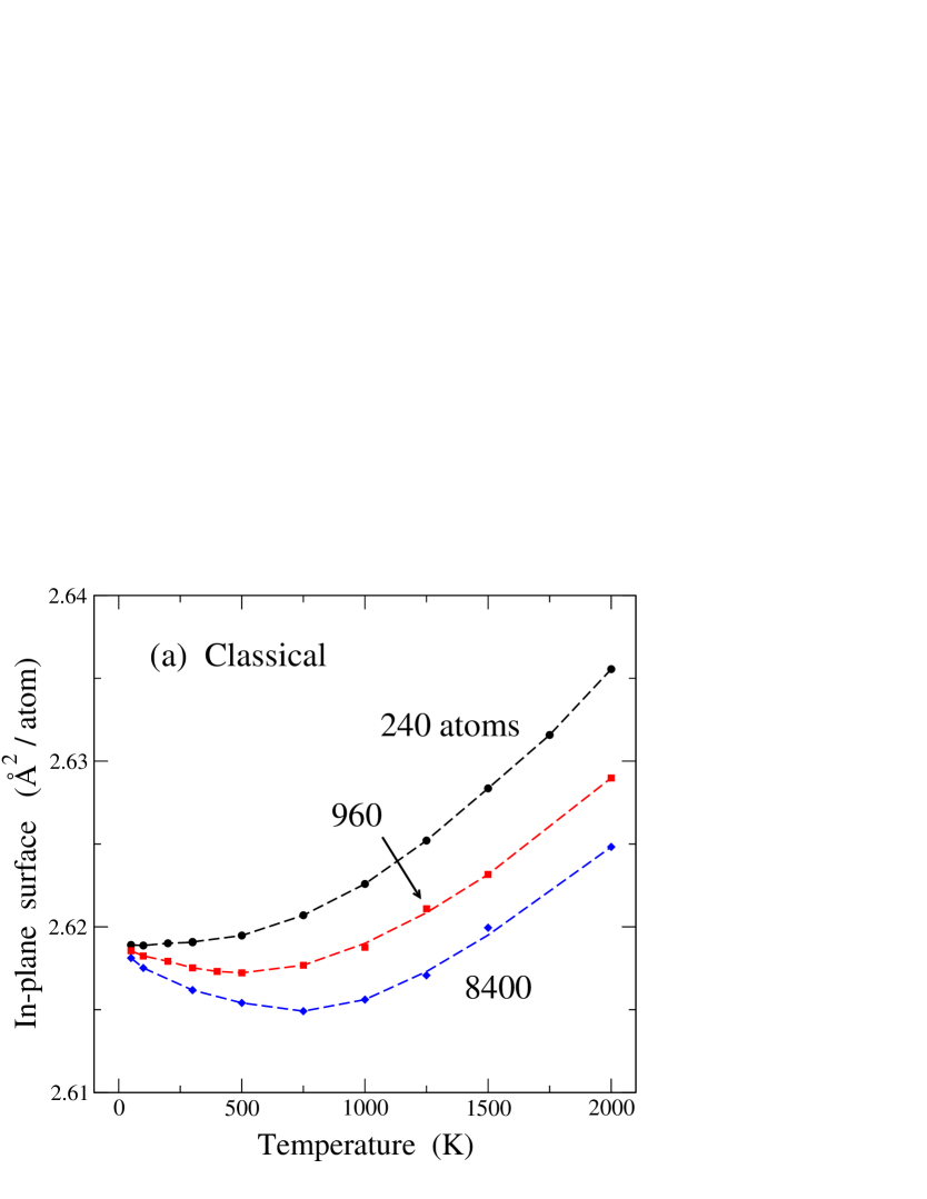
In Fig. 2 we display the temperature dependence of the in-plane area associated to the graphene layer, as derived from (a) classical MD and (b) PIMD simulations. In each plot, results for three cell sizes are given: = 240 (circles), 960 (squares), and 8400 (diamonds) atoms. Let us look first at the results of the classical simulations in Fig. 2(a). For the larger sizes (960 and 8400 atoms) one observes first a decrease in for rising , and at higher temperatures increases with . For the smallest size presented here, the low-temperature decrease in is also present, although almost unobservable in the figure. Moreover, one sees that the normalized in-plane surface per atom is smaller for larger simulation cells. These results are similar to those found in earlier classical Monte Carlo and MD simulations of graphene single layers.Zakharchenko et al. (2009); Gao and Huang (2014); Brito et al. (2015) There are two competing effects which explain this temperature dependence of , as discussed below.
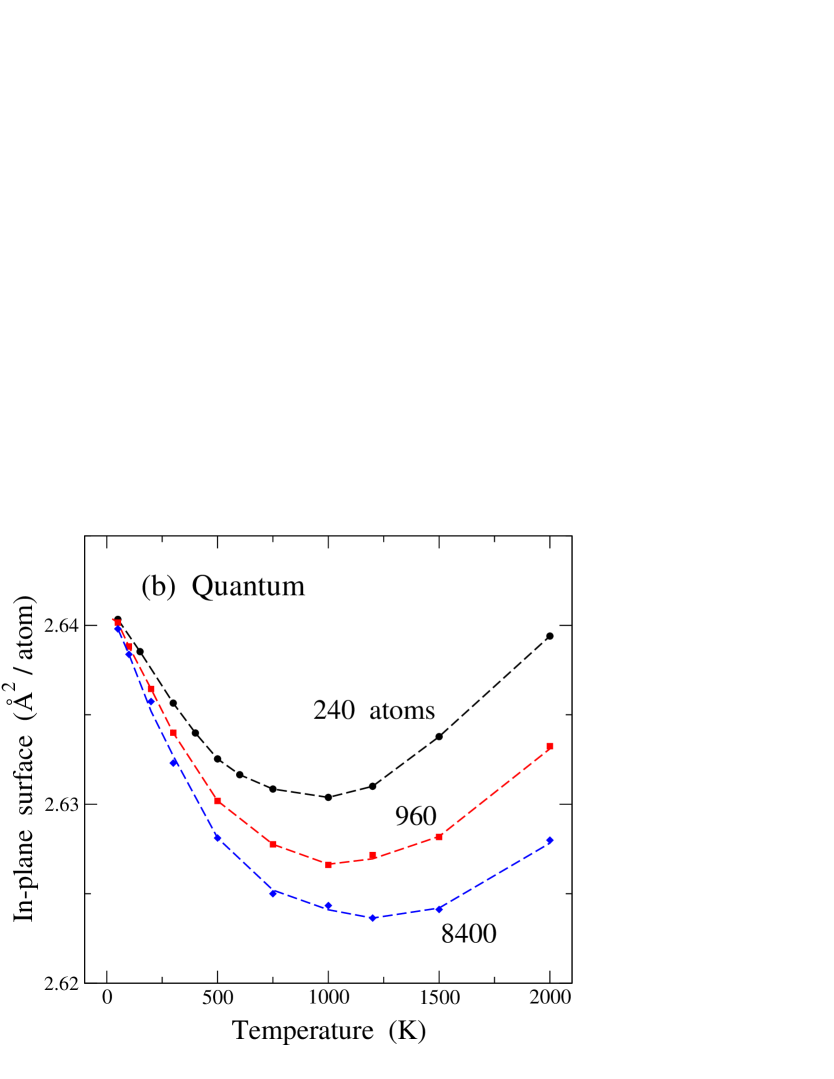
In Fig. 2(b) we present the temperature dependence of , as derived from PIMD simulations, for the same cell sizes as in Fig. 2(a). This dependence is qualitatively similar to that corresponding to the classical results, but in the quantum simulations the low-temperature decrease of the in-plane area is more pronounced. This is particularly visible for the smallest size presented here ( = 240), for which such a decrease in for rising is almost inappreciable in the classical results, whereas it is clearly visible in the results of the quantum simulations. It is important to note that, in spite of the large differences in the in-plane area per atom for the different system sizes, in each case (classical or quantum) all sizes converge at low to a single value. This could be expected because for the graphene sheet becomes strictly planar in the classical case and close to planar in the quantum model (a zero-point effect).
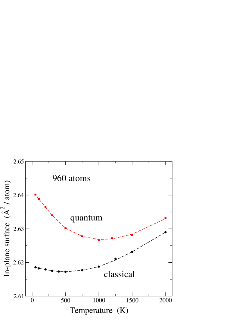
For a direct comparison of the in-plane area obtained from classical and quantum simulations, we show in Fig. 3 both sets of results for system size = 960. In the limit , the difference between them converges to 0.022 Å2. This difference decreases for rising temperature, as nuclear quantum effects become less relevant. For this system size, the overall behavior of vs is similar for both classical and quantum models, in the sense that at low temperature and this derivative becomes positive at high . However, the slope of the vs curve at low temperature is much larger for the quantum than for the classical model.
In view of the results shown in Fig. 3, it seems that could not vanish for , in disagreement with the third law of thermodynamicsCallen (1960); Wallace (1972) (This apparent inconsistency is however not real, as shown below in Sec. IV). Moreover, one can ask if can be treated as a true extensive variable, given that it shows a strong size effect, as shown in Fig. 2. In any case, one can use as a helpful variable to carry out simulations of layered systems such as graphene, and indeed it is which defines the area of the simulation cell in the plane. This in-plane area has been studied earlier in several worksGao and Huang (2014); Brito et al. (2015); Zakharchenko et al. (2009); Los et al. (2016); Chacón et al. (2015) as a function of temperature and external stress, but one can argue that it is not necessarily a variable to which one can associate properties of a real material surface.
This can be further illustrated by considering a “real” surface (in 3D space) for graphene, as can be defined from the actual bonds between carbon atoms. Thus, we define a mean area per atom from the mean C–C distance derived from the simulations, as (see Fig. 7 in Ref. Ramírez et al., 2016). A similar expression has been used by Hahn et al.Hahn et al. (2016) to study nanocrystalline graphene from atomistic simulations. As the actual interatomic distance changes from bond to bond in a simulation step and for each bond it fluctuates along a simulation run, is a mean value for a given temperature, and fluctuations of the instantaneous area depend on the fluctuations of the interatomic distance. One could employ alternative definitions for the real area, based for example on the areas of the hexagons that make up the graphene sheet, or on a triangulation based on the atomic positions. We have checked that such definitions yield area values slightly smaller than the area defined above, but in the present conditions (zero applied stress and not very large out-of-plane fluctuations) this difference is not relevant for our current purposes.
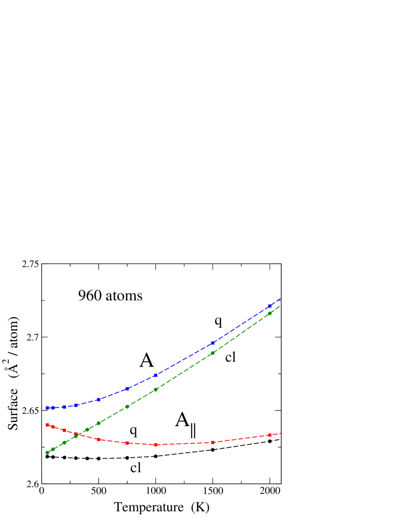
In Fig. 4 we show the areas and vs temperature for a simulation cell including 960 atoms. In both cases, we present results from classical and PIMD simulations. The surface is larger than , and the difference between both increases with temperature. In fact, is the 2D projection of , and the actual surface becomes increasingly bent as temperature is raised and out-of-plane atomic displacements are larger. For the area we do not observe the anomalous decrease displayed by in both classical and quantum cases at low temperature. Moreover, the area derived from quantum simulations shows a temperature derivative approaching zero as , in agreement with low-temperature thermodynamics.
For the classical results, we find that both surfaces and converge one to the other in the low- limit, as expected for a convergence of the actual graphene surface to a plane when out-of-plane atomic displacements go to zero as . In the quantum case, and become closer as temperature is reduced, but in the low- limit is still larger than , and the extrapolated difference amounts to Å2/atom for . This difference is due to the fact that even for the graphene layer is not strictly planar due to zero-point motion of the carbon atoms in the out-of-plane direction.
We now discuss the behavior of as a function of , with at relatively low temperature. There appears a competition between two opposite factors. On one side, the actual area increases as temperature is raised, as shown in Fig. 4 for both classical and quantum simulations. On the other side, bending (rippling) of the surface causes a decrease in its 2D projection, i.e., in . At low , the decrease associated to out-of-plane motion dominates the thermal expansion of the actual surface, and thus . This is particularly marked for the quantum results, because in this case the thermal expansion at low is very small. At high temperature, the increase in dominates the reduction in the projected area associated to out-of-plane atomic displacements. For example, for the classical results, increases roughly linearly with , but the mean-square atom displacements (causing the reduction of ) grow up slower than linearly, as a consequence of anharmonicity. This is in line with the discussion given by Gao and HuangGao and Huang (2014) for the thermal behavior of observed in classical MD simulations of a single graphene layer, as well as with the trends for calculated by Michel et al.Michel et al. (2015a)
The discussion of a real area and a projected area presented here is reminiscent of the analysis carried out earlier in the context of biological membranes, where consideration of a “true” area is important to describe some properties of those membranes.Chacón et al. (2015) In fact, it has been shown that values of the membrane compressibility may be very different when they are related to or to . Something similar can happen for graphene, and this topic requires further research.
To summarize the results of this section, we emphasize that changes in interatomic distances and in the graphene area (both and ) are important anharmonic effects. On one side, changes in the distance and in the real area are mainly due to anharmonicity of the C-C stretching vibration. The dilation of the C-C bond displayed in Fig. 1 equally appears in a strictly planar graphene, and shows a temperature dependence similar to that of interatomic distances in solids. In real graphene, will be also affected by out-of-plane vibrations, which in fact couple with in-plane vibrational modes, but this coupling changes less than the only anharmonicity of the in-plane modes, at least for the conditions considered here. Something different occurs for the projected area , as manifested by the strong size effect which it displays. In this case, the coupling between in-plane and out-of-plane modes is crucial to understand the temperature dependence of in the absence of an external stress (). The amplitude of out-of-plane vibrations strongly depend on the size ,Gao and Huang (2014) causing the large size effect in . At low temperatures, all these anharmonic effects are clearly enhanced by quantum motion, as shown for example in Fig. 3 for the projected area. This is due to the fact that anharmonicity is manifested in the quantum model even in the limit , contrary to the classical case, where it gradually appears as temperature is raised. This is further quantified and discussed in the next section.
III.3 Vibrational energy
In the zero-temperature limit we find in the classical approach a strictly planar graphene surface with an interatomic distance of 1.4199 Å. This corresponds to fixed atomic nuclei on the equilibrium sites without spatial delocalization, defining a minimum energy , taken as a reference for our calculations. In the quantum approach, the low-temperature limit includes out-of-plane atomic fluctuations due to zero-point motion, so that the graphene layer is not strictly planar, as commented above. Moreover, anharmonicity of in-plane vibrations cause a slight zero-point bond expansion, giving an interatomic distance of 1.4287 Å, as shown in Fig. 1.
We now turn to the results of our simulations at finite temperatures, and will discuss the resulting energy for graphene. The internal energy, , at temperature can be written as:
| (6) |
where is the elastic energy corresponding to an area , and is the vibrational energy of the system. Our simulations directly yield in both classical and quantum approaches. We can then split the internal energy into an elastic and a vibrational part.
To define the elastic energy corresponding to an area , we have carried out calculations of the (classical) energy of a supercell including 960 atoms, expanding it isotropically and keeping it flat. This strict 2D atomic layer gives us a reference to evaluate the vibrational energy. The elastic energy increases with , and for small expansion it can be approximated as , with = 2.41 eV/Å2. For the area derived from our classical and PIMD simulations at 300 K, we found elastic energies of 0.4 and 2.8 meV/atom, respectively. This much larger value for the quantum approach is a consequence of the larger surface , as compared to the classical limit at = 300 K. Those values of the elastic energy increase to 20.8 and 22.9 meV/atom at 2000 K.
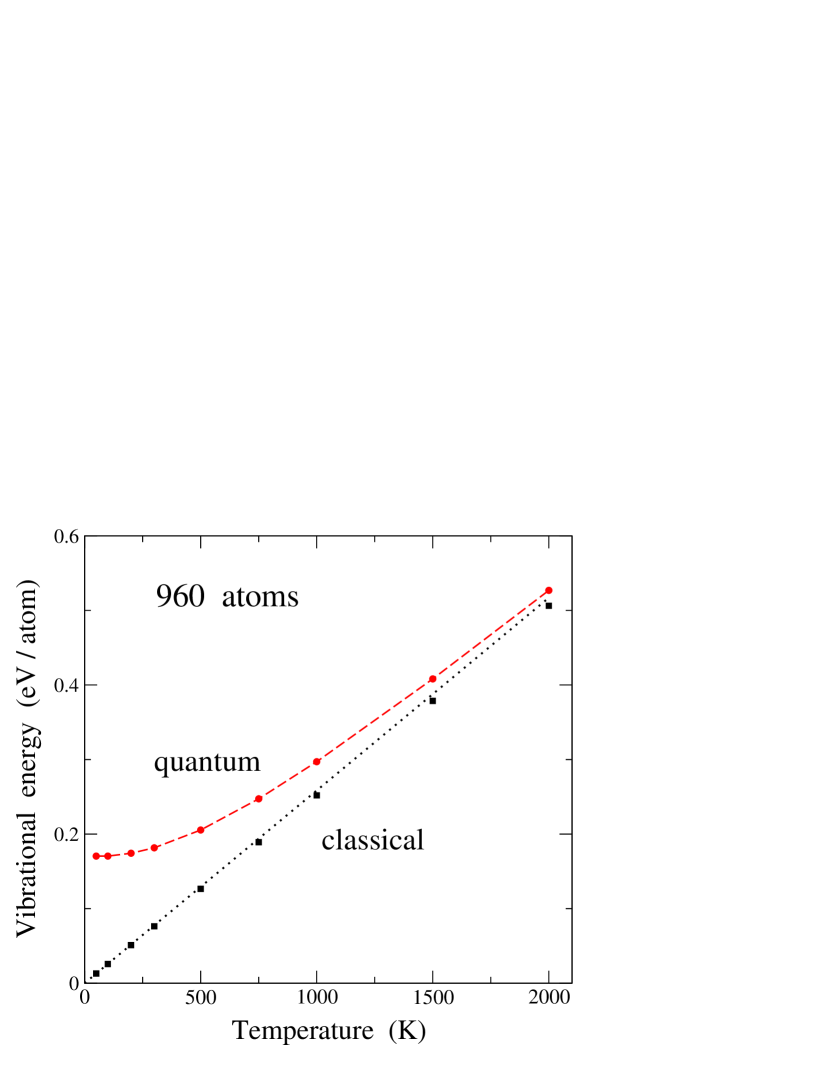
Thus, we obtain the vibrational energy from the results of our simulations by subtracting in each case the elastic energy from the internal energy . In Fig. 5 we show the temperature dependence of , derived from simulations for a supercell including 960 carbon atoms. At 300 K, the vibrational energy amounts to 182 meV/atom, somewhat smaller than the values reported for diamond of 195 and 210 meV/atom, yielded by path-integral simulations with Tersoff-type and tight-binding potentials, respectively.Herrero and Ramírez (2000); Ramírez et al. (2006) This has to be compared to the value expected in a classical harmonic approximation: = 77.6 meV/atom ( is Boltzmann’s constant). Note also that the elastic energy in the quantum approach at 300 K is 1.5% of the internal energy , most of this energy corresponding to the vibrational energy .
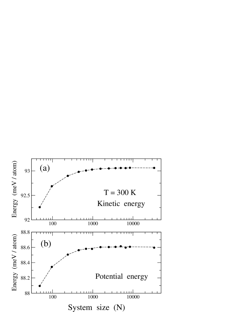
PIMD simulations allow us to separate the potential () and kinetic () contributions to the vibrational energy,Herman et al. (1982); Giansanti and Jacucci (1988); Gillan (1990) so that . In the classical limit, the kinetic energy amounts to per atom. In the quantum case, however, depends on the spatial delocalization of the quantum paths, which can be obtained from the simulations as indicated above [see Eq. (3)]. In our simulations of graphene, both kinetic and potential energy were found to slightly increase with system size, but their convergence is rather fast. In Fig. 6, we present and derived from PIMD simulations as a function of cell size at = 300 K. Symbols indicate results of our simulations for [panel (a)] and [panel (b)], whereas dashed lines are guides to the eye. In both and there appears a shift of less than 1 meV/atom when increasing the cell size from 40 atoms to the largest size considered here (about 30,000 atoms). For cells in the order of 1000 atoms the size effect is almost inappreciable when compared to the largest cell. The potential energy is found to be smaller than the kinetic energy, indicating an appreciable anharmonicity of the lattice vibrations (see below).
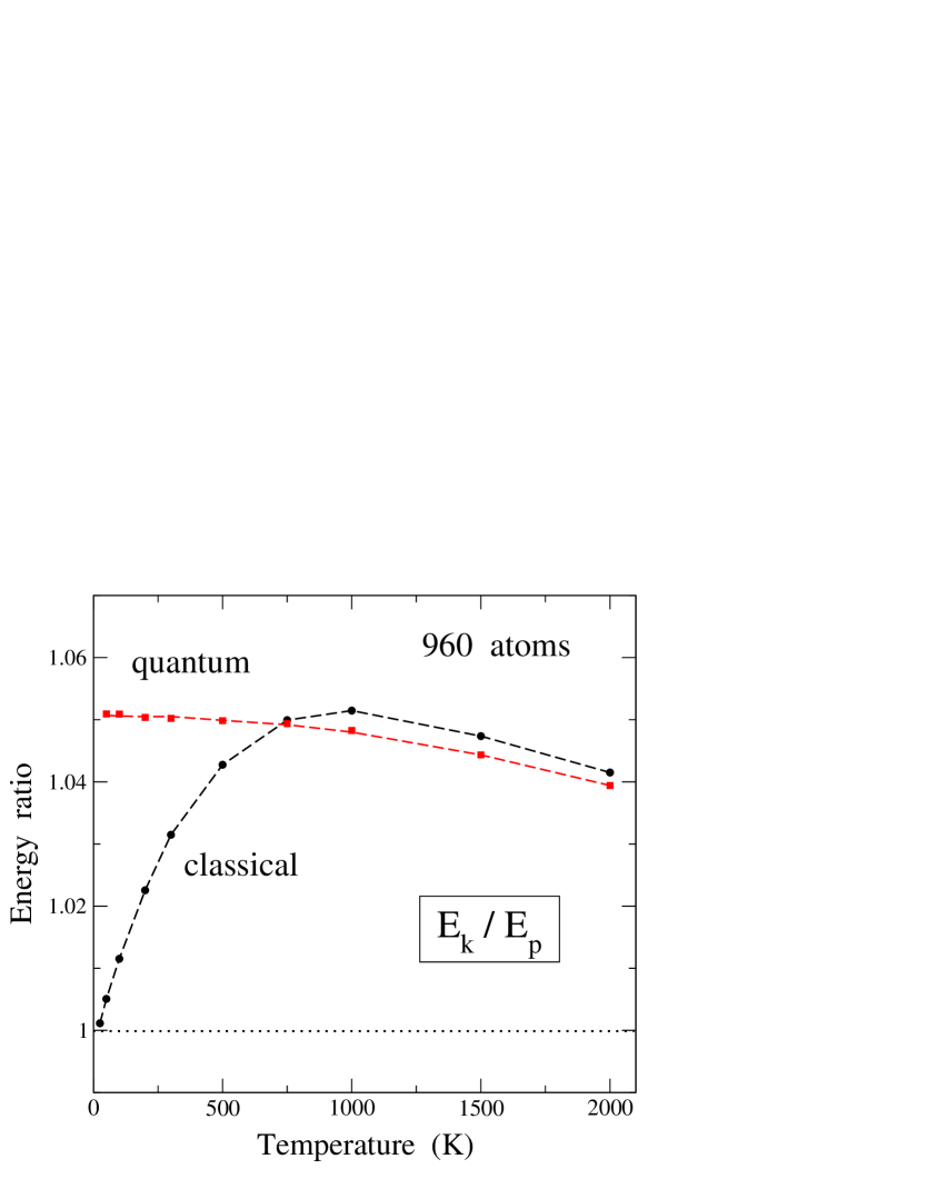
Differences between the kinetic and potential contribution to the vibrational energy can be used for a quantification of the anharmonicity in condensed matter, as has been discussed earlier from path-integral simulations, e.g., for H impurities in siliconHerrero and Ramírez (1995) and van der Waals solids.Herrero (2002) In Fig. 7 we display the ratio between kinetic and potential parts of the vibrational energy of graphene as a function of temperature. Results are shown for classical (circles) and PIMD (squares) simulations carried out for a system size = 960 atoms. The effect of system size on the energy ratio is a slight shift in both cases, classical and quantum, as can be derived from results such as those presented in Fig. 6.
For a purely harmonic model for the vibrational modes, one expects (virial theoremLandau and Lifshitz (1980); Feynman (1972)), i.e., an energy ratio equal to unity at any temperature in both classical and quantum approaches. The ratio is found in the classical model for the low-temperature limit, since in this case the atomic motion does not feel the anharmonicity of the interatomic interactions, due to the vanishingly small vibrational amplitudes. This is not the case of the quantum results for , because now the vibrational amplitudes remain finite and feel the anharmonicity. In particular, we find , and at low temperature this ratio amounts to about 1.05. In the classical model, increases at low , due to an enhancement of vibrational amplitudes, as in this approach the mean-square atomic displacements increase at low linearly with rising temperature. This increase in the energy ratio continues until about = 1000 K, and at higher temperatures is found to decrease, close to the quantum result. This slow decrease for rising obtained for the energy ratio from both classical and PIMD simulations does not mean that the difference decreases (in fact it rises with ), but is due to the large increase in the denominator . Also, for 1000 K the ratio turns out to be larger for the classical case than in the quantum approach, even though the difference is similar in both cases, because in the classical approach is smaller.
Turning to the energy results for the quantum approach at , it is interesting to note that earlier analysis of anharmonicity in solids, based on quasiharmonic approximations and perturbation theory indicate that low-temperature changes in the vibrational energy with respect to a harmonic calculation are mainly due to the kinetic energy. In fact, assuming perturbed harmonic oscillators (with perturbations of or type) at , the first-order change in the energy is caused by changes in , the potential energy remaining unaltered with respect to its unperturbed value.Landau and Lifshitz (1965); Herrero and Ramírez (1995)
III.4 Atomic motion: Out-of-plane displacements
In this section we present results for the mean-square displacements of carbon atoms in graphene, as obtained from our PIMD simulations. We mainly focus on the character of these atomic displacements, i.e., if they can be described by a classical model, or the C atoms mainly behave as quantum particles. One obviously expects that the quantum description will become more relevant as the temperature is lowered, but we show that the system size also plays an important role in this question. We use the notation introduced in Sec. II.
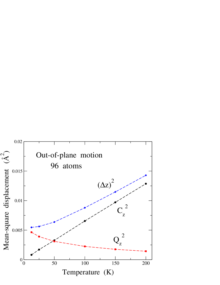
In Fig. 8 we display results for the motion in the out-of-plane direction , derived for a cell including 96 atoms. Diamonds represent the mean-square displacement as a function of temperature [see Eq. (2)]. As explained above, this displacement can be split into two parts: one of them properly quantum in nature, corresponding to the spread of the quantum paths, (squares), and another of semiclassical character, taking into account the centroid motion, i.e., global displacements of the paths, (circles). In the limit , vanishes and converges to a value of about Å2. decreases for increasing temperature, whereas increases almost linearly with . For the system size shown in Fig. 8 (N = 96), both contributions to are nearly equal at = 50 K. At higher temperatures, the semiclassical part is the main contribution to the atomic displacements on the out-of-plane direction. Values of obtained from our PIMD simulations coincide within error bars with the mean-square atomic displacement in the direction obtained from classical MD simulations. The proper quantum delocalization can be estimated from the mean extension of the quantum paths in the direction, i.e., from . At 25 and 300 K we find an average extension 0.06 and 0.03 Å, respectively.
The vibrational amplitudes in the layer plane are smaller than in the direction. This is true for both, quantum and classical contributions. In the limit , zero-point motion yields a mean-square displacement on the plane Å2, which means = = Å2. Thus, for each direction in the plane we find a value about three times smaller than the zero-point mean-square displacement in the direction. This is due, of course, to the low-frequency out-of-plane modes, which cause a larger vibrational amplitude. At finite temperatures, the difference between vibrational amplitudes in-plane and out-of-plane are larger than at . At 300 K, we find = 11.9 and 61.8 for simulation cells with 96 and 960 atoms, respectively. This is a consequence of the appearance of long-wavelength modes (with low frequency) with larger vibrational amplitudes in the larger cells, as explained below.
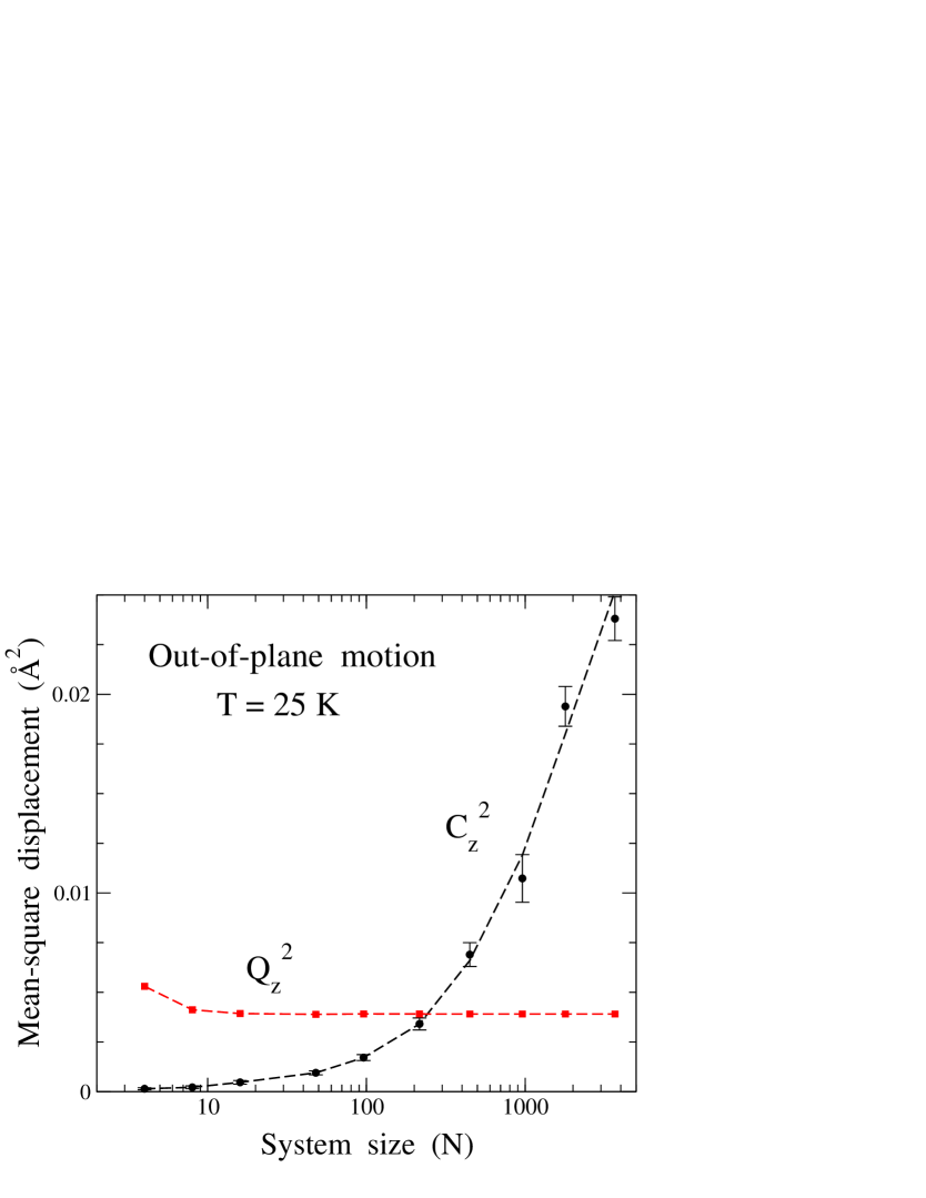
The picture shown in Fig. 8 for the atom displacements in the direction is qualitatively the same for different system sizes, but the temperature region where or is the main contribution to is strongly dependent on the system size . This is mainly due to the enhancement of the classical-like contribution for increasing size, a fact already observed and described earlier from results of classical MD simulations.Los et al. (2009); Gao and Huang (2014); Ramírez et al. (2016) In Fig. 9 we present mean-square displacements and in the out-of-plane direction at = 25 K for different . One observes that the quantum contribution converges fast as is increased, and in fact for , changes in are much smaller than the symbol size. Clear finite-size effects are only observed for very small simulation cells. The semiclassical contribution is small for small , and grows with system size, so that at = 25 K it becomes similar to for . Calling the system size at which and are equal, we found that decreases for rising temperature, and for 50 K we have [see Fig. 8].
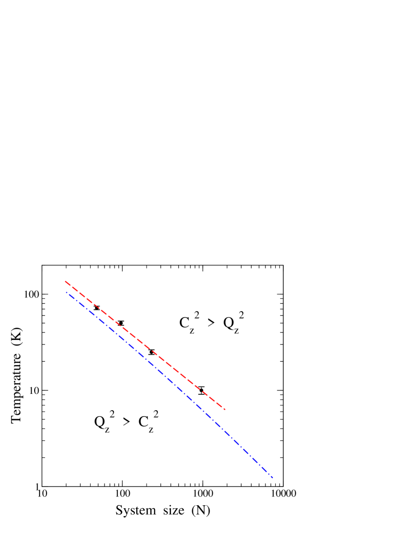
On the other side, for a given system size , the ratio decreases for increasing , and there is a crossover temperature for which this ratio is unity. For classical-like motion dominates the atomic mean-square displacement in the direction. In Fig. 10 we show as a function of the system size . Symbols are results derived from our PIMD simulations. The dashed line through the data points was obtained as a linear fit of vs for the crossover temperatures derived from the simulations for several cell sizes. This is consistent with a power-law dependence of the crossover temperature on system size, i..e, with a factor K and an exponent .
This means that for a given temperature (even very low), there is a system size for which classical-like motion along the out-of-plane direction dominates over atomic quantum delocalization. Thus, extrapolating the dashed line in Fig. 10, we find for = 1 K and 0.1 K crossover sizes and , respectively. These values are much larger than the simulation cells which can be dealt with in PIMD simulations at low temperatures. We note, however, that the dependence of on may depart from the power-law given above (dashed line in Fig. 10) for larger system sizes. This is related to the size dependence of , which has been proposed to increase logarithmically with (from an atomistic model for the spectral amplitudesGao and Huang (2014); Ramírez et al. (2016)) or as a power-law (based on a scaling theory in the continuum medium approachLos et al. (2009)). In any case, this difference would be detected for system sizes much larger than those considered here in the PIMD simulations.
This can be rationalized in terms of vibrational modes in the direction appearing for different system sizes. The mean-square displacements and can be estimated in a harmonic approximation in the following way. The classical part is given by:
| (7) |
where is the atomic mass and the sum is extended to the wavevectors in the reciprocal lattice corresponding to the two-dimensional simulation cell.Ramírez et al. (2016) This expression is valid for relatively low temperatures, as for high anharmonic effects cause to rise sublinearly with .Gao and Huang (2014) On the other side, in the limit , converges to
| (8) |
Increasing the system size causes the appearance of vibrational modes with longer wavelength . In fact, one has an effective cut-off , with . Calling , this translates into , i.e., . We consider a dispersion relation of the form , consistent with an atomic description of grapheneRamírez et al. (2016) (, surface mass density; , effective stress; , bending modulus). Then, the sum in Eq. (7) diverges in the large-size limit due to the term in the denominator and the two-dimensional character of the wavevector Gao and Huang (2014); Ramírez et al. (2016) (see results for vs at 25 K in Fig. 9). However, the sum in Eq. (8) converges to a finite value for large , in agreement with the results of our PIMD simulations at low temperature (see results for vs in Fig. 9).
Given a temperature , modes with frequency may be considered in the classical regime. Then, increasing one reaches a system size for which any further increase introduces new modes with frequency , and therefore contributing to increase the classical displacement more than the quantum one . Thus, at any finite temperature classical-like displacements will dominate over quantum delocalization in the out-of-plane direction, provided that the system size is larger than the corresponding .
All this can be visualized in terms of the harmonic model. Taking into account that at low temperatures , the dispersion relation in the direction is (see Ref. Ramírez et al., 2016). At temperature , the mean-square displacement can be approximated as
| (9) |
Then, from Eqs. (7) and (9), and remembering that , we calculate for each the temperature at which . This yields the curve shown as a dashed-dotted line in Fig. 10, displaying a dependence of on very similar to that derived from PIMD simulations for system sizes accessible in our calculations. In fact, for , the results can be approximated in both cases by a power-law with nearly the same exponent. For larger sizes, the harmonic calculation deviates to temperatures somewhat smaller than the extrapolation of the simulation data. At this point, we cannot assure if this deviation is a real trend of the physical system or only a consequence of the harmonic approach. The main limitations of this approximation are the neglect of anharmonicity in the vibrational modes (expected to be reasonably small at low ) and the overestimation of frequencies in the -space region far from the point (k = 0). In that region, increases with slower than (see Ref. Mounet and Marzari, 2005; Michel et al., 2015b; Ramírez et al., 2016). Even with these limitations the harmonic model captures qualitatively, and almost quantitatively, the basic aspects of the competition between classical-like and proper quantum dynamics of the carbon atoms in the direction.
We finally note that the competition between and as a function of discussed here appears only in the direction. For motion in the plane, both and converge fast with increasing system size to their asymptotic value, similarly to the behavior known for vibrational motion in 3D solids.Herrero and Ramírez (2014)
IV Thermodynamic consistency
Here we analyze the thermodynamic consistency of the results of our PIMD simulations. In particular, we discuss their compatibility with the third law of thermodynamics. According to this law, some variables such as the heat capacity or thermal expansion should vanish in the limit .Callen (1960); Wallace (1972)
Concerning the heat capacity derived from the PIMD simulations, we find for all system sizes considered here low-temperature values compatible with the third law, i.e. for . This can be visualized in Fig. 5, where the vibrational energy obtained from PIMD simulations fulfills at low . Something similar happens for the elastic energy , so that the temperature derivative of the internal energy [see Eq. (6)] also vanishes at low . This is similar to the results of earlier path-integral simulations of 3D solids,Herrero and Ramírez (2000, 2014) where the resulting data were in agreement with the basic laws of thermodynamics.
A more subtle question appears for the thermal expansion of graphene. We first note that, following our definitions of 3D area and in-plane area , we consider two different definitions for the areal thermal expansion coefficient:
| (10) |
and
| (11) |
The 3D area derived from our PIMD simulations displays a negligible size effect, as indicated in Sec. III.B. Therefore, the same happens for the coefficient , which vanishes in the zero-temperature limit and is found to be positive at all finite temperatures considered here (see Fig. 4).
Concerning the in-plane area , we have shown that there appears a strong size effect in both classical and quantum results (see Fig. 2). Moreover, for both kinds of simulations the data shown in Figs. 2 and 3 seem to indicate that the in-plane thermal expansion coefficient is negative at low temperature, irrespective of the cell size. This causes no particular problems for the classical results, as discussed above. However, in the quantum case, one should expect a vanishing at temperatures low enough to have all vibrational modes (nearly) in their ground state, so that the system is “frozen” and no change in could occur.
A hint to solve this apparent inconsistency can be obtained from the discussion in Sec. III.D concerning the vibrational modes appearing effectively for each cell size. The relevant modes for this purpose are the low-frequency out-of-plane modes (in the direction), since in-plane modes have much larger frequencies. The results summarized in Fig. 10 indicate that the temperature region where proper quantum motion dominates over classical-like motion in the direction is strongly dependent on the system size. Thus, for = 240 (the smallest size shown in Fig. 2), one has to go to K to observe the mode “freezing” mentioned above.
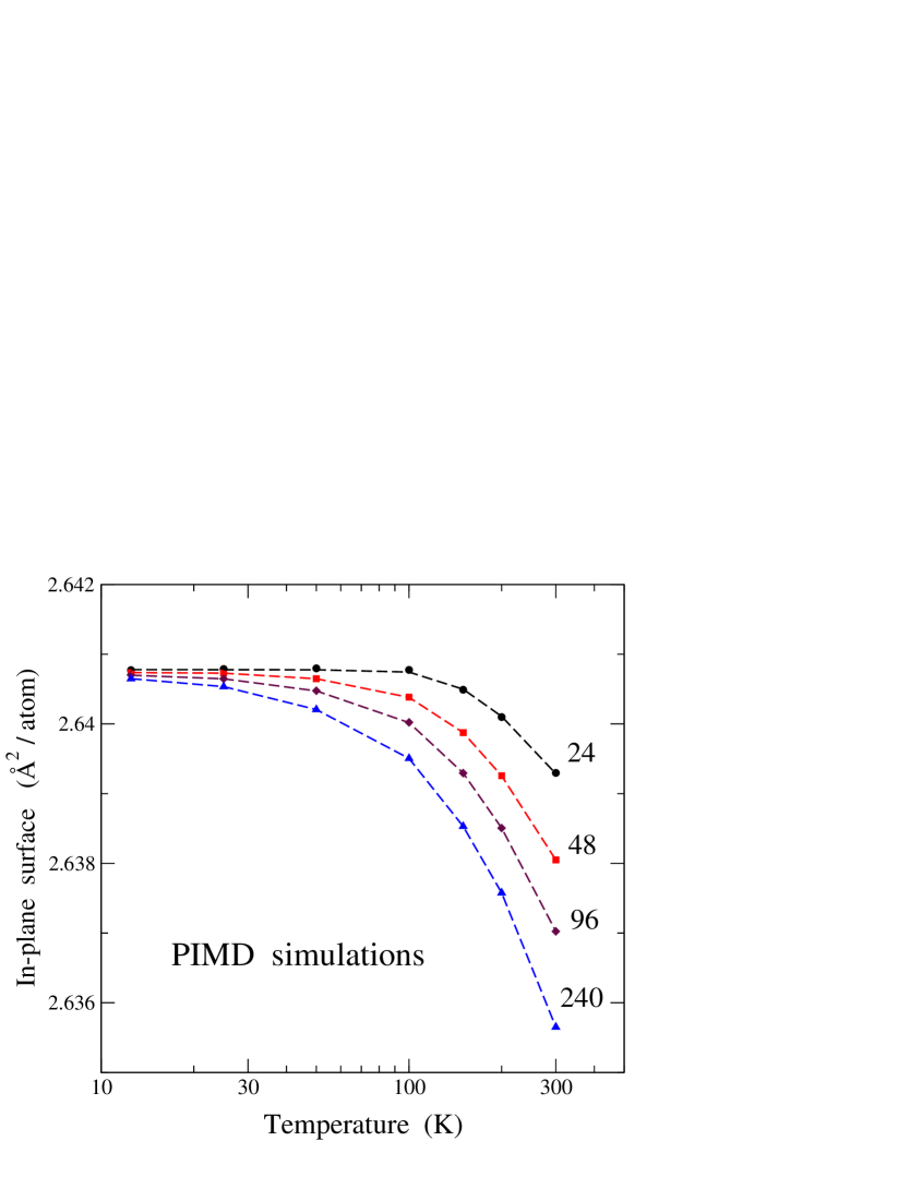
Since the temperature for this “freezing” to occur increases by reducing the cell size, making it more readily appreciable, we have carried out some PIMD simulations for cell sizes and temperatures down to = 24 and = 12 K. The results for are displayed in Fig. 11 in a semilogarithmic plot, including system sizes of 24, 48, 96, and 240 atoms. In all cases we find that the curve becomes flat at low temperature, as expected for a vanishing of , but this is more manifest for smaller sizes, in agreement with Fig. 10. Moreover, converges to the same value for the different cell sizes: = 2.6408 Å2/atom. For = 240 one observes that saturates at low to the same value as the smaller cell sizes, although this is almost inappreciable at the scale of Fig. 2(b).
These low-temperature data for are consistent with the trend in the low-temperature limit derived by Amorim et al.,Amorim et al. (2014) who investigated the thermodynamic properties of 2D crystalline membranes using a first-order perturbation theory and a one-loop self-consistent approximation. These authors also found that the limits and do commute, a fact compatible with the results shown in Fig. 11, i.e., at low all system sizes yield the same results. We find, however, that an evaluation of the low-temperature (quantum) properties becomes harder in both limits. Going to larger does not only mean to increase the system size, but to reduce the temperature to reach the proper quantum regime, with the consequent increase in the Trotter number appearing in PIMD simulations.
V Summary
In this paper we have presented results of PIMD simulations of a graphene monolayer in the isothermal-isobaric ensemble at several temperatures and zero external stress. The relevance of quantum effects has been assessed by comparing results given by PIMD simulations with those yielded by classical MD simulations. Structural variables are found to change when quantum nuclear motion is taken into account, especially at low temperatures. Thus, the sheet area and interatomic distances change appreciably in the range of temperatures considered here.
The LCBOPII potential model is known to describe fairly well various structural and thermodynamic properties of carbon-like materials, and graphene in particular. Here we have investigated its reliability to study effects related to the quantum character of atomic nuclei, and their vibrational motion in particular. Given the ability of this effective potential to describe rather accurately the vibrational frequencies of graphene, one expects that quantum effects associated to vibrational motion should be equally described in a reliable manner by PIMD simulations using this potential. The results obtained in the simulations have allowed us to propose a consistent interpretation of the in-plane () and “real” () graphene surfaces. In order to check these finite-temperature results, it would be desirable to study structural and thermodynamic properties of graphene from an ab-initio method. This is, however, not feasible at present for the large supercells required to study these properties.
Particular emphases has been laid on the atomic vibrations along the out-of-plane direction. Even though quantum effects are present in these vibrational modes, we have shown that at any finite temperature classical-like motion dominates over quantum delocalization, provided that the system size is large enough. This size effect is present in the quantum simulations at low temperatures, as a consequence of the appearance of vibrational modes with smaller wavenumbers in larger graphene cells. Moreover, by comparing the kinetic and potential energy derived from PIMD simulations, we have shown that vibrational modes display a nonnegligible anharmonicity, even for . This comparison indicates that the overall kinetic energy is larger than the vibrational potential energy by about 5% at low temperatures.
An important question related to the overall consistency of the simulation results is their agreement with the basic principles of thermodynamics. This is usually taken for granted in the standard simulation methods used today, but in the case of graphene some subtle questions may appear due to its 2D character in a 3D world. In particular, the third law of thermodynamics has to be satisfied, in the sense that proper thermodynamic variables should display at low temperature a behavior compatible with this law, e.g., thermal expansion coefficients should converge to zero for . We have shown that this requirement is fulfilled by both the in-plane area and the 3D area derived from PIMD simulations.
In summary, we have shown that (1) the so-called thermal contraction of graphene mentioned in the literature is in fact a reduction of the projected area due to out-of-plane vibrations, and not a to an actual decrease in the real area of the graphene sheet. (2) The difference between and increases for rising due to the larger amplitude of those vibrations. (3) Zero-point expansion of the graphene layer due to nuclear quantum effects is not negligible, and it amounts to an increase of about 1% in the area . (4) The temperature dependence of the projected area may be qualitatively different when derived from classical or PIMD simulations, even at temperatures between 300 and 1000 K (see Fig. 3). (5) Anharmonicity of the vibrational modes is appreciable and should be taken into account in any finite-temperature calculation of the properties of graphene. (6) The temperature region where out-of-plane vibrational modes are predominantly of quantum character decreases as the system size rises. This is important for a comparison of results derived from classical and quantum models for different system sizes. (7) Thermodynamic consistency of the results of PIMD simulations at low has been shown.
Path-integral simulations similar to those presented here may help to understand low-temperature properties of a hydrogen monolayer on graphene (graphane). Also, the dynamics of free-standing graphene multilayers may display interesting quantum features at low temperature.
Acknowledgements.
The authors acknowledge the support of J. H. Los in the implementation of the LCBOPII potential, and E. Chacón is thanked for inspiring discussions. This work was supported by Dirección General de Investigación, MINECO (Spain) through Grants FIS2012-31713 and FIS2015-64222-C2References
- Geim and Novoselov (2007) A. K. Geim and K. S. Novoselov, Nat. Mater. 6, 183 (2007).
- Flynn (2011) G. W. Flynn, J. Chem. Phys. 135, 050901 (2011).
- Castro Neto et al. (2009) A. H. Castro Neto, F. Guinea, N. M. R. Peres, K. S. Novoselov, and A. K. Geim, Rev. Mod. Phys. 81, 109 (2009).
- Meyer et al. (2007) J. C. Meyer, A. K. Geim, M. I. Katsnelson, K. S. Novoselov, T. J. Booth, and S. Roth, Nature 446, 60 (2007).
- Fasolino et al. (2007) A. Fasolino, J. H. Los, and M. I. Katsnelson, Nature Mater. 6, 858 (2007).
- Kim and Castro Neto (2008) E.-A. Kim and A. H. Castro Neto, EPL 84, 57007 (2008).
- Amorim et al. (2016) B. Amorim, A. Cortijo, F. de Juan, A. G. Grushin, F. Guinea, A. Gutiérrez-Rubio, H. Ochoa, V. Parente, R. Roldán, P. San-Jose, et al., Phys. Reports 617, 1 (2016).
- Katsnelson and Geim (2008) M. I. Katsnelson and A. K. Geim, Phil. Trans. R. Soc. A 366, 195 (2008).
- Guinea et al. (2008) F. Guinea, M. I. Katsnelson, and M. A. H. Vozmediano, Phys. Rev. B 77, 075422 (2008).
- de Andres et al. (2012a) P. L. de Andres, F. Guinea, and M. I. Katsnelson, Phys. Rev. B 86, 144103 (2012a).
- Warner et al. (2013) J. H. Warner, Y. Fan, A. W. Robertson, K. He, E. Yoon, and G. D. Lee, Nano Lett. 13, 4937 (2013).
- Wei et al. (2013) Y. Wei, B. Wang, J. Wu, R. Yang, and M. L. Dunn, Nano Lett. 13, 26 (2013).
- Mermin (1968) N. D. Mermin, Phys. Rev. 176, 250 (1968).
- Safran (1994) S. A. Safran, Statistical Thermodynamics of Surfaces, Interfaces, and Membranes (Addison Wesley, New York, 1994).
- Nelson et al. (2004) D. Nelson, T. Piran, and S. Weinberg, Statistical Mechanics of Membranes and Surfaces (World Scientific, London, 2004).
- Tarazona et al. (2013) P. Tarazona, E. Chacón, and F. Bresme, J. Chem. Phys. 139, 094902 (2013).
- Pop et al. (2012) E. Pop, V. Varshney, and A. K. Roy, MRS Bull. 37, 1273 (2012).
- Fong et al. (2013) K. C. Fong, E. E. Wollman, H. Ravi, W. Chen, A. A. Clerk, M. D. Shaw, H. G. Leduc, and K. C. Schwab, Phys. Rev. X 3, 041008 (2013).
- Amorim et al. (2014) B. Amorim, R. Roldan, E. Cappelluti, A. Fasolino, F. Guinea, and M. I. Katsnelson, Phys. Rev. B 89, 224307 (2014).
- Wang et al. (2016) P. Wang, W. Gao, and R. Huang, J. Appl. Phys. 119, 074305 (2016).
- Shimojo et al. (2008) F. Shimojo, R. K. Kalia, A. Nakano, and P. Vashishta, Phys. Rev. B 77, 085103 (2008).
- de Andres et al. (2012b) P. L. de Andres, F. Guinea, and M. I. Katsnelson, Phys. Rev. B 86, 245409 (2012b).
- Chechin et al. (2014) G. M. Chechin, S. V. Dmitriev, I. P. Lobzenko, and D. S. Ryabov, Phys. Rev. B 90, 045432 (2014).
- Cadelano et al. (2009) E. Cadelano, P. L. Palla, S. Giordano, and L. Colombo, Phys. Rev. Lett. 102, 235502 (2009).
- Herrero and Ramírez (2009) C. P. Herrero and R. Ramírez, Phys. Rev. B 79, 115429 (2009).
- Akatyeva and Dumitrica (2012) E. Akatyeva and T. Dumitrica, J. Chem. Phys. 137, 234702 (2012).
- Lee et al. (2013) G.-D. Lee, E. Yoon, N.-M. Hwang, C.-Z. Wang, and K.-M. Ho, Appl. Phys. Lett. 102, 021603 (2013).
- Los et al. (2009) J. H. Los, M. I. Katsnelson, O. V. Yazyev, K. V. Zakharchenko, and A. Fasolino, Phys. Rev. B 80, 121405 (2009).
- Shen et al. (2013) H.-S. Shen, Y.-M. Xu, and C.-L. Zhang, Appl. Phys. Lett. 102, 131905 (2013).
- Magnin et al. (2014) Y. Magnin, G. D. Foerster, F. Rabilloud, F. Calvo, A. Zappelli, and C. Bichara, J. Phys.: Condens. Matter 26, 185401 (2014).
- Los et al. (2016) J. H. Los, A. Fasolino, and M. I. Katsnelson, Phys. Rev. Lett. 116, 015901 (2016).
- Ramírez et al. (2016) R. Ramírez, E. Chacón, and C. P. Herrero, Phys. Rev. B 93, 235419 (2016).
- Gillan (1988) M. J. Gillan, Phil. Mag. A 58, 257 (1988).
- Ceperley (1995) D. M. Ceperley, Rev. Mod. Phys. 67, 279 (1995).
- Brito et al. (2015) B. G. A. Brito, L. Cândido, G.-Q. Hai, and F. M. Peeters, Phys. Rev. B 92, 195416 (2015).
- Calvo and Magnin (2016) F. Calvo and Y. Magnin, Eur. Phys. J. B 89, 56 (2016).
- Mounet and Marzari (2005) N. Mounet and N. Marzari, Phys. Rev. B 71, 205214 (2005).
- Shao et al. (2012) T. Shao, B. Wen, R. Melnik, S. Yao, Y. Kawazoe, and Y. Tian, J. Chem. Phys. 137, 194901 (2012).
- Gao and Huang (2014) W. Gao and R. Huang, J. Mech. Phys. Solids 66, 42 (2014).
- Herrero and Ramírez (2000) C. P. Herrero and R. Ramírez, Phys. Rev. B 63, 024103 (2000).
- Ramírez et al. (2006) R. Ramírez, C. P. Herrero, and E. R. Hernández, Phys. Rev. B 73, 245202 (2006).
- Herrero and Ramírez (2007) C. P. Herrero and R. Ramírez, Phys. Rev. Lett. 99, 205504 (2007).
- Herrero and Ramírez (2010) C. P. Herrero and R. Ramírez, Phys. Rev. B 82, 174117 (2010).
- Kwon and Ceperley (2012) Y. Kwon and D. M. Ceperley, Phys. Rev. B 85, 224501 (2012).
- Feynman (1972) R. P. Feynman, Statistical Mechanics (Addison-Wesley, New York, 1972).
- Kleinert (1990) H. Kleinert, Path Integrals in Quantum Mechanics, Statistics and Polymer Physics (World Scientific, Singapore, 1990).
- Chandler and Wolynes (1981) D. Chandler and P. G. Wolynes, J. Chem. Phys. 74, 4078 (1981).
- Herrero and Ramírez (2014) C. P. Herrero and R. Ramírez, J. Phys.: Condens. Matter 26, 233201 (2014).
- Los and Fasolino (2003) J. H. Los and A. Fasolino, Phys. Rev. B 68, 024107 (2003).
- Los et al. (2005) J. H. Los, L. M. Ghiringhelli, E. J. Meijer, and A. Fasolino, Phys. Rev. B 72, 214102 (2005).
- Ghiringhelli et al. (2008) L. M. Ghiringhelli, C. Valeriani, J. H. Los, E. J. Meijer, A. Fasolino, and D. Frenkel, Mol. Phys. 106, 2011 (2008).
- Ghiringhelli et al. (2005a) L. M. Ghiringhelli, J. H. Los, A. Fasolino, and E. J. Meijer, Phys. Rev. B 72, 214103 (2005a).
- Zakharchenko et al. (2009) K. V. Zakharchenko, M. I. Katsnelson, and A. Fasolino, Phys. Rev. Lett. 102, 046808 (2009).
- Zakharchenko et al. (2010) K. V. Zakharchenko, J. H. Los, M. I. Katsnelson, and A. Fasolino, Phys. Rev. B 81, 235439 (2010).
- Zakharchenko et al. (2011) K. V. Zakharchenko, A. Fasolino, J. H. Los, and M. I. Katsnelson, J. Phys.: Condens. Matter 23, 202202 (2011).
- Ghiringhelli et al. (2005b) L. M. Ghiringhelli, J. H. Los, E. J. Meijer, A. Fasolino, and D. Frenkel, Phys. Rev. Lett. 94, 145701 (2005b).
- Politano et al. (2012) A. Politano, A. R. Marino, D. Campi, D. Farías, R. Miranda, and G. Chiarello, Carbon 50, 4903 (2012).
- Lambin (2014) P. Lambin, Appl. Sci. 4, 282 (2014).
- Tuckerman et al. (1992) M. E. Tuckerman, B. J. Berne, and G. J. Martyna, J. Chem. Phys. 97, 1990 (1992).
- Tuckerman and Hughes (1998) M. E. Tuckerman and A. Hughes, in Classical and Quantum Dynamics in Condensed Phase Simulations, edited by B. J. Berne, G. Ciccotti, and D. F. Coker (Word Scientific, Singapore, 1998), p. 311.
- Martyna et al. (1999) G. J. Martyna, A. Hughes, and M. E. Tuckerman, J. Chem. Phys. 110, 3275 (1999).
- Tuckerman (2002) M. E. Tuckerman, in Quantum Simulations of Complex Many–Body Systems: From Theory to Algorithms, edited by J. Grotendorst, D. Marx, and A. Muramatsu (NIC, FZ Jülich, 2002), p. 269.
- Martyna et al. (1996) G. J. Martyna, M. E. Tuckerman, D. J. Tobias, and M. L. Klein, Mol. Phys. 87, 1117 (1996).
- Herrero et al. (2006) C. P. Herrero, R. Ramírez, and E. R. Hernández, Phys. Rev. B 73, 245211 (2006).
- Herrero and Ramírez (2011) C. P. Herrero and R. Ramírez, J. Chem. Phys. 134, 094510 (2011).
- Herman et al. (1982) M. F. Herman, E. J. Bruskin, and B. J. Berne, J. Chem. Phys. 76, 5150 (1982).
- Ramírez et al. (2012) R. Ramírez, N. Neuerburg, M. V. Fernández-Serra, and C. P. Herrero, J. Chem. Phys. 137, 044502 (2012).
- Gillan (1990) M. J. Gillan, in Computer Modelling of Fluids, Polymers and Solids, edited by C. R. A. Catlow, S. C. Parker, and M. P. Allen (Kluwer, Dordrecht, 1990), p. 155.
- Callen (1960) H. B. Callen, Thermodynamics (John Wiley, New York, 1960).
- Wallace (1972) D. C. Wallace, Thermodynamics of crystals (John Wiley, New York, 1972).
- Pozzo et al. (2011) M. Pozzo, D. Alfè, P. Lacovig, P. Hofmann, S. Lizzit, and A. Baraldi, Phys. Rev. Lett. 106, 135501 (2011).
- Yamanaka et al. (1994) T. Yamanaka, S. Morimoto, and H. Kanda, Phys. Rev. B 49, 9341 (1994).
- Ramdas et al. (1993) A. K. Ramdas, S. Rodriguez, M. Grimsditch, T. R. Anthony, and W. F. Banholzer, Phys. Rev. Lett. 71, 189 (1993).
- Kazimorov et al. (1998) A. Kazimorov, J. Zegenhagen, and M. Cardona, Science 282, 930 (1998).
- Chacón et al. (2015) E. Chacón, P. Tarazona, and F. Bresme, J. Chem. Phys. 143, 034706 (2015).
- Hahn et al. (2016) K. R. Hahn, C. Melis, and L. Colombo, J. Phys. Chem. C 120, 3026 (2016).
- Michel et al. (2015a) K. H. Michel, S. Costamagna, and F. M. Peeters, Phys. Status Solidi B 252, 2433 (2015a).
- Giansanti and Jacucci (1988) A. Giansanti and G. Jacucci, J. Chem. Phys. 89, 7454 (1988).
- Herrero and Ramírez (1995) C. P. Herrero and R. Ramírez, Phys. Rev. B 51, 16761 (1995).
- Herrero (2002) C. P. Herrero, Phys. Rev. B 65, 014112 (2002).
- Landau and Lifshitz (1980) L. D. Landau and E. M. Lifshitz, Statistical Physics (Pergamon, Oxford, 1980), 3rd ed.
- Landau and Lifshitz (1965) L. D. Landau and E. M. Lifshitz, Quantum Mechanics (Pergamon, Oxford, 1965), 2nd ed.
- Michel et al. (2015b) K. H. Michel, S. Costamagna, and F. M. Peeters, Phys. Rev. B 91, 134302 (2015b).