Quantum error correction using weak measurements
Abstract
The standard quantum error correction protocols use projective measurements to extract the error syndromes from the encoded states. We consider the more general scenario of weak measurements, where only partial information about the error syndrome can be extracted from the encoded state. We construct a feedback protocol that probabilistically corrects the error based on the extracted information. Using numerical simulations of one-qubit error correction codes, we show that our error correction succeeds for a range of the weak measurement strength, where (a) the error rate is below the threshold beyond which multiple errors dominate, and (b) the error rate is less than the rate at which weak measurement extracts information. It is also obvious that error correction with too small a measurement strength should be avoided.
pacs:
03.67.Pp, 03.65.YzI Introduction
In recent years, the field of quantum information and quantum computation has rapidly progressed from a theoretical framework to an experimental level, where toy systems carry out simple but practical tasks. The main hurdle to be overcome for large scale integration of quantum devices is a control over errors. No physical system can be perfectly isolated from the environment, and the inevitable disturbances affect its operation. Quantum information processors are especially sensitive in this regard, and designs that would make them fault-tolerant are an outstanding challenge. A recent road map for fault-tolerant quantum computation Devoret and Schoelkopf (2013) emphasizes the role that quantum error correction (QEC) would have to play to protect the quantum data. The QEC strategy is to redundantly encode the quantum information in a larger Hilbert space, such that the logical qubits experience a significantly smaller error rate than what the physical qubits do. A cascade of QEC codes can then make the lifetime of encoded quantum information as long as desired.
The standard QEC codes are illustrated by the label . They encode logical qubits into physical qubits, and is the minimum distance between logical codewords. The errors are discretized to a finite set in the Pauli operator basis for each qubit, they are detected using projective measurements of the appropriate syndromes, and then the measurement-result-dependent inverse transformations restore the original information. This procedure corrects upto Pauli errors, and the residual error rate of the encoded state is given by the probability of having more than errors. The procedure is worthwhile only when the error rate of -qubit encoded state is smaller than the error rate of -qubit unencoded state, and that happens only when the error rate of unencoded state is below a critical threshold. Such codes were first devised by Shor Shor (1995) and Steane Steane (1996), and a variety of them have been constructed since then. For practical applications, it is paramount to understand the error mechanisms as well as possible, and then design the codes to maximize the critical threshold. Attempts to build quantum error correction procedures for several physical systems have been made, e.g. liquid Cory et al. (1998); Knill et al. (2001); Boulant et al. (2005) and solid state Moussa et al. (2011) NMR, trapped ions Chiaverini et al. (2004); Schindler et al. (2011), photon modes Pittman et al. (2005), superconducting qubits Reed et al. (2012); Kelly et al. (2015), and NV centers in diamond Waldherr et al. (2014); Taminiau et al. (2014).
Projective measurements are instantaneous, they extract maximum information about the measured observable, and their post-measurement state is known with certainty. These properties allow accurate error correction. In contrast, weak measurements are performed on a stretched out time scale, with only a gentle disturbance to the quantum system Aharonov et al. (1988). They extract only partial information about the measured observable, which rules out complete error correction. With weak measurements, therefore, we can only aim to restore the quantum state with as high fidelity as possible. In this work, we present a protocol to implement quantum error correction using weak measurements. Obviously, it would be useful only when projective measurements cannot be carried out for some reason.
Attempts to construct QEC protocols using weak measurements have been made before Ahn et al. (2002); Sarovar et al. (2004). In our work, we use continuous stochastic measurement dynamics to design a QEC feedback protocol. We propose a general feedback scheme based on binary weak measurements, and numerically investigate its efficacy as a function of the measurement coupling. Our protocol is appropriate for weak measurements of superconducting transmon qubits, but it can be easily extended to other physical systems.
This paper is organized as follows. Section II briefly reviews how a quantum system evolves during weak measurement, using the setting of circuit QED, and presents our feedback scheme for a quantum register when all measurements are binary weak measurements. Section III describes the numerical simulation results of our protocol, for the bit-flip error correction of a single qubit encoded in a three-qubit register, and arbitrary error correction of a single qubit encoded in a five-qubit register. We conclude with a discussion of our results in Section IV.
II Weak measurements and feedback
A quantum system interacting with the environment and the measuring apparatus undergoes a complex evolution. We omit any driving term, e.g. the system could be some quantum information stored in memory, and model the total evolution as:
| (1) |
Here and are the error and the feedback Hamiltonians respectively, and are the projectors for the measured observable. Compared to the usual framework for QEC codes Nielsen and Chuang (2000), we have replaced the projective measurement evolution, , with the weak measurement evolution operator .
We use the framework of continuous quantum stochastic dynamics to describe weak measurements Gisin (1984). In this framework, an ensemble of quantum trajectories is generated, by combining geodesic evolution of the initial quantum state to the eigenstates of the measured observable with white noise fluctuations. In this evolution, every quantum trajectory keeps a pure state pure (i.e. preserves ), and the Born rule is satisfied at every instant of time (upon averaging over the stochastic noise). We use the notation Patel and Kumar (2015):
| (2) |
where the system-apparatus interaction parameter has dimensions of energy ( can be time-dependent, in which case in the rest of the article should be interpreted as ). vanishes at the fixed points , ensuring termination and repeatability of measurements. The weights are normalized to . They are chosen such that the system’s dynamics reproduces the well-established quantum behaviour, and the weak measurement contributes a stochastic noise to Korotkov (1999, 2001); Vijay et al. (2012); Murch et al. (2013). The projective measurement is recovered in the limit .
II.1 Binary measurement
For a binary weak measurement,
| (3) |
where is a white noise with and . During weak measurement, can be experimentally observed along any quantum trajectory.
In recent years, weak measurements have been implemented experimentally for superconducting transmon qubits Vijay et al. (2012); Murch et al. (2013). A transmon qubit is essentially a tunable nonlinear quantum oscillator made of two Josephson junctions in a superconducting loop shunted by a capacitor. The lowest two energy levels of the nonlinear oscillator are used as a qubit. The qubit is kept in a microwave cavity with dispersive coupling, and its weak measurements are carried out by probing the cavity by a microwave signal. For weak measurement of a transmon, the signal observed by the apparatus is a current , and is obtained by scaling it suitably. We adopt the convention that the ideal measurement current is for the measurement eigenstates and . Then the scaled measurement current, , provides an estimate of .
The redundancy of the encoding QEC protocol allows extraction of the syndrome information from the encoded state without disturbing the encoded information. The simplest code to correct a single bit-flip error encodes the logical qubit into three physical qubits. Parities of qubit-pairs provide the syndrome information, which is extracted into two additional ancilla qubits, using -NOT logic gates as illustrated in Fig.1. These parities are then used to apply controlled inverse logic operations to eliminate the error. (For the sake of simplicity, we have assumed that all gate operations are perfect, and the qubits are exposed to the error perturbations only before the measurement and feedback steps. A more elaborate fault-tolerant prescription can take care of errors occurring anywhere during the evolution.) After using the parities for the feedback, the ancilla qubits need to be disentangled from the encoded state, and that is achieved by resetting the ancilla qubits. This resetting is an irreversible step, and it reduces the fidelity of the encoded quantum state. Different methods have been proposed for resetting the ancilla qubits Reed et al. (2010); Geerlings et al. (2013), and they can be applied equally well after strong or weak measurements.

II.2 Feedback design
Initially the quantum system is in the logical subspace. Under the influence of undesired disturbances, it moves out of the logical subspace along some of the error directions. The syndrome operators are designed to reveal the information about the error without disturbing the encoded signal. The binary syndrome operators have a eigenvalue for the logical subspace and a eigenvalue for some of the error states. The complete error information is constructed from a collection of binary syndrome measurements.
The measurement evolution, described by Eqs. (1,2,3), can be expressed in the Itô form as Gisin (1984):
| (4) | |||||
| (5) |
Here the stochastic Wiener increment obeys and . For any initial state , the time evolution of the quantum trajectory distribution is known Gisin (1984). After time , the initial -function distribution becomes a sum of two Gaussians with areas and , centered at and respectively, and with a common variance .
The unperturbed logical space state has or . Due to errors,
the state gets shifted to some finite , and the feedback task is to
move it back to . The syndrome measurement is designed to estimate
, but ends up shifting the state more in the process. To figure out what
feedback to apply, with only incomplete information available, we make the
following approximations:
(i) We approximate the measurement evolution as a binary walk on a line,
producing -function distributions at with probabilities
and . For each step of a quantum trajectory, only one of the two
possibilities occur, i.e. the post-measurement state is either or
. Of course, is known from the properties of the measurement
apparatus.
(ii) The current measured by the apparatus provides an average value of the
signal over the measurement duration; so we use to
estimate either or .
(iii) The measured current is a combination of
and white noise. We next assume that if
then the post-measurement state is , and if
then the post-measurement state is .
With these assumptions, we convert into a rotation angle on the Bloch sphere, and design the feedback transformation. When , the act of measurement moves the state from to , which is closer to the logical subspace corresponding to . We then opt to apply no additional feedback operation. When , we construct the feedback operation as follows. In terms of polar coordinates on the Bloch sphere,
| (6) |
We estimate the post-measurement state location as,
| (7) | |||||
Here the replacement of by is the most severe approximation, due to which the last line of the previous equation is not restricted to the interval . Whenever the value goes outside this interval, we replace it by corresponding to the value being less than or greater than respectively.
The rotation angle represents the combined shift of the quantum state due to error and measurement. This shift can be reversed by applying an inverse rotation by . The binary measurement does not determine the polar angle of the shift on the Bloch sphere. To estimate , knowledge of off-diagonal elements of is needed, which is not available to us. (In case of projective measurements, and ignorance of does not matter.) Knowledge of is necessary to decide around which axis in the X-Y plane the feedback rotation should be applied. Without that knowledge, we ad hoc choose the X-axis as the rotation axis. Consequently, the feedback may correct the error or may make it worse. Whenever the error gets worse, it would become easier to detect, and then to correct, in the next iteration. We hope that the procedure converges with repeated error correction steps with high fidelity, and our simulation results support that.
In weak measurements, the measured current, given by Eq.(3), is a noisy current. We can reduce the noise, and hence increase the accuracy of Eq.(7), by accumulating the signal over as long evolution time as possible:
| (8) |
Use of the integrated current as the signal, instead of the original current , is tantamount to using a stronger interaction strength . Also, a non-uniform integration weight in the definition of would lose some information, and so is not worthwhile. Once the feedback has been applied, then we have to erase all the current history, and wait until ample new current data is accumulated, before deciding on the next feedback operation. All this is equivalent to saying that we apply feedback only when we have sufficient information, and don’t disturb the system otherwise.
II.3 Multiple binary measurements
Now consider the situation where the syndrome consists of two commuting binary measurements, and and are the corresponding measured currents. The physical Hilbert space can be divided into four sectors corresponding to the measurement projectors , , , , where the superscript denotes the measurement number. For each binary measurement, we determine the rotation angle as in the previous subsection:
| (9) |
where denotes reduction of the value to the interval , as described after Eq.(7). The feedback operation is then constructed from these angles. The syndrome definition tells us the location of the error in the multi-qubit register; so we determine the location of the error from the signs of . For -measurements, we do not have knowledge of the polar angles , and as before, we ad hoc choose the -axis as the rotation axis.
When all the are positive, we do not apply any feedback operation. When only one of the is negative, we use the inverse rotation as the feedback operation. When more than one are negative, assuming each to be an equal diagnostic of the error, we estimate movement of the state out of the logical subspace by averaging the corresponding . The feedback operation is then the inverse rotation obtained from the averaged projection. For instance, when and ,
| (10) |
This is an empirical prescription, but numerically we find it to be a good approximation.
III Numerical simulations and results
We have performed numerical simulations to ascertain the accuracy of our feedback scheme. Various terms on the r.h.s. of the evolution equation (1) contribute simultaneously in reality. For ease of simulation, however, we calculate these contributions one by one for evolution time , and then combine them together. As per Trotter’s formula, the error incurred in this procedure is , and we make that inconsequential by choosing to be sufficiently small.
Within time step , the system evolution is broken up into three parts: (1) evolution under error, (2) evolution under measurement, and (3) evolution under feedback. For evolution under error, we evolve Eq.(1) using the fourth order Runge-Kutta method and only the contribution.
We then include the effect of measurement by performing a probabilistic Bayesian update Korotkov (2011) that effectively integrates Eq.(2). The measurement current is drawn from Gaussian probability distributions centered at and with standard deviations . Explicitly, the conditional probability distributions for the measurement current, when the system is in or state, are Vijay et al. (2012):
| (11) |
With these conditional distributions, the probability distribution for the measurement current is,
| (12) |
For a binary measurement of an -dimensional system, all that appear in are updated as Korotkov (2001):
| (13) |
while all that appear in are updated as:
| (14) |
All the off-diagonal are updated according to the unitary evolution constraint,
| (15) |
Finally, we apply the feedback transformation described in the previous section, by converting the rotation into the feedback Hamiltonian , and evolving Eq.(1) with only the contribution.
III.1 Single qubit bit-flip error correction
Consider a single qubit system initialized in the state that undergoes a bit-flip error. The error Hamiltonian is
| (16) |
where is the Pauli operator representing the bit-flip error, and the error coupling is chosen as a Gaussian random number with zero mean and variance . (We choose this form of as a likely scenario in actual experiments.) Evolution under the error Hamiltonian for time changes the state of the system as
| (17) |
where . For a system initialized in the state , Eq.(17) simplifies to
| (18) |
Averaging over the distribution of the error coupling , the averaged density matrix becomes:
| (19) | |||||
Fidelity of the quantum state evolves as
| (20) |
and eventually the system reaches the completely mixed state.
Choosing as a Gaussian random variable is an assumption, and the error distribution may be different in a different experimental setting. As another example, we consider the binary error distribution case, again with zero mean and variance . Then the error coupling is either or with equal probability. In this case, the averaged density matrix after time evolution becomes:
| (21) |
and the fidelity is
| (22) |
Although we use the Gaussian error distribution in our simulations throughout this work, we note that the choice between the Gaussian or the binary error distribution does not matter much for small values of , both giving essentially the same fidelity as shown in Fig. 2.
To protect a single qubit system against bit-flip error, we redundantly encode it in a three-qubit register as:
| (23) |
The states and are basis vectors of the logical space, while and are basis vectors of the physical space. A general logical state to be protected is
| (24) |
with . In our simulations, we have chosen the initial state as to simplify calculations; the linearity of evolution ensures that when the protocol works for the basis states, it will also work for any superposition of basis states. Our measured fidelity of the encoded state is thus
| (25) |
We diagnose the bit-flip errors using the syndrome operators (i.e. ) and (i.e. ).
In the three-qubit Hilbert space, the independent bit-flip error Hamiltonian is:
| (26) |
where the error couplings are independent Gaussian random numbers with zero mean and variance .
Let the measurement currents for and be and respectively. We take the feedback Hamiltonian to be
| (27) |
where are the feedback couplings. We estimate the feedback rotation angles as described in Section II.C. The feedback couplings are then:
| (28) | |||||
In case of projective measurement (i.e. ), , and the fidelity of the quantum state after applying the feedback can be analytically determined as:
| (29) |
From Eqs. (20) and (29), we find that
and therefore projective measurement error correction always improves fidelity, irrespective of the value of .
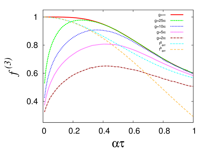
In our simulations, we varied (by holding fixed and varying ), and observed how fidelity changes as the measurement strength is varied. Our results, averaged over trajectories to cut down the statistical errors, are shown in Fig. 2. We observe that for large , the fidelity approaches the result obtained by performing projective measurement error correction. For small , the measurement current fluctuates heavily, leading to uncertain feedback that spoils the fidelity. Increasing reduces these fluctuations, and the measurement accumulates sufficient information to improve fidelity. As a consequence, it is not desirable to perform error correction when is rather small.
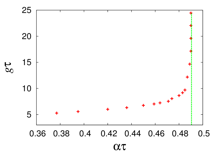
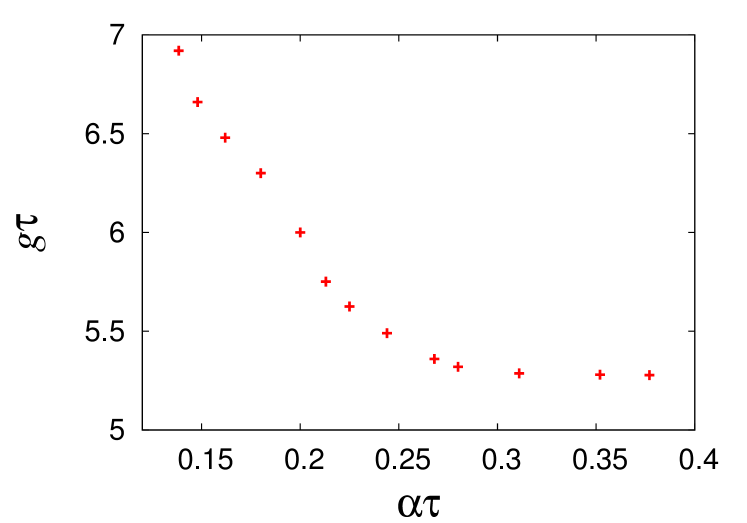
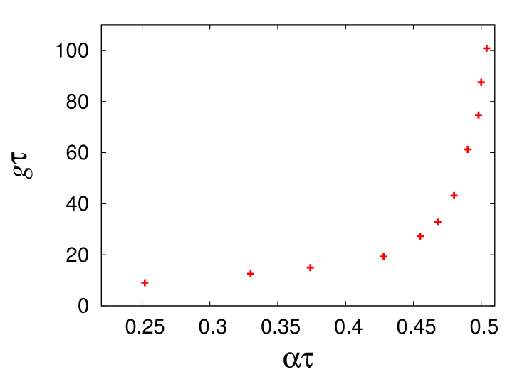
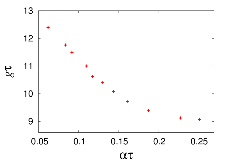
It can also be observed from Fig. 2 that fidelity improvement varies, depending on the relative strengths of and . To illustrate that, we have plotted respectively in Figs. 3, 4, the upper and lower bounds on for different values of , between which reduces by at least a factor of two after applying error correction. These two bounds arise for different physical reasons, and can be understood as follows.
When the measurement coupling decreases, we need to evolve the system for long to accumulate sufficient information. Within the same duration, to keep the overall error under control, we need to decrease . As a result, the upper bound on decreases with decreasing , as displayed in Fig. 3 (this effect is implicit in Fig. 2). For projective measurement error correction, the upper bound on , calculated analytically using Eqs.(20) and (29), is 0.4905. Fig. 3 shows that approaches this value as we increase . Beyond this threshold, multiple errors overwhelm the error correction process and prevent improvement in fidelity.
The lower bound on results from the error correction protocol becoming noisy, when inadequate information is extracted by the weak measurement. In case of projective measurement, the post-measurement state is known precisely, which allows perfect error correction. But for smaller , it is difficult to accurately estimate the qubit state from the measurement current (the approximations described in Section II.B become far from precise), unless it is sufficiently perturbed by a large . Consequently the lower bound on increases with decreasing , as displayed in Fig. 4 (this effect is also visible in Fig. 2).
From our results, we find that the two bounds on meet around . Attempts to correct errors with smaller values of are pointless; the best option in such situations is not to perform any error correction.
III.2 Single qubit arbitrary error correction
In the previous subsection, we described how to correct single bit-flip errors. But a complete quantum error correction protocol has to correct all errors that may occur. For a single qubit, the complete error Hamiltonian can be written as:
| (30) |
Here represents a bit-flip error, represents a phase-flip error, and represents both of them occurring together. We take the error couplings to be independent Gaussian random numbers with zero mean and variance . Assuming that the system is initialized in the state , the density matrix after evolution with the error Hamiltonian for time becomes,
| (31) |
when averaged over the distributions of . The fidelity of the quantum state therefore evolves as
| (32) |
If the error distribution is taken to be a binary distribution, instead of a Gaussian distribution, the averaged density matrix becomes
| (33) |
which has the fidelity
| (34) |
For small values of , Eqs.(32) and (34) give almost the same fidelity as depicted in Fig. 5, and the choice of error distribution doesn’t matter much.
To protect the single logical qubit from arbitrary error, we encode it in a five-qubit physical register Laflamme et al. (1996); Bennett et al. (1996), according to Preskill :
| (35) |
where . In our simulations, without loss of generality, we choose the initial state to be , which makes our measured fidelity of the encoded state
| (36) |
We diagnose all single Pauli errors using the four syndrome operators:
| (37) |
For the five-qubit register, the independent error Hamiltonian can be written as:
| (38) | |||||
where the error couplings are independent Gaussian random numbers with zero mean and variance .
Our feedback Hamiltonian is:
| (39) | |||||
where are the feedback couplings. With four different binary syndrome measurements, there are 16 possible outcomes. The one with all four currents positive stands for “no error”, while the other 15 possibilities correspond to single qubit errors. Different combinations of the measured currents determine the corresponding non-zero , as listed in the following table.
| Non-zero | ||||
|---|---|---|---|---|
| + | + | + | - | |
| - | + | + | + | |
| - | - | + | + | |
| + | - | - | + | |
| + | + | - | - | |
| - | + | - | - | |
| - | - | + | - | |
| - | - | - | + | |
| - | - | - | - | |
| + | - | - | - | |
| - | + | - | + | |
| + | - | + | - | |
| + | + | - | + | |
| - | + | + | - | |
| + | - | + | + |
We estimate the feedback rotation angle by extending the procedure described in Section II.C to four binary measurements. At every evolution step, only one (or none) of the fifteen feedback couplings is non-zero, determined by its unique syndrome signature. The non-zero rotation angle always equals .
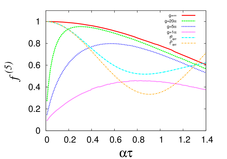
In our simulations, we once again varied (by holding fixed and varying ), and observed how the fidelity changes as the measurement strength varies. Our results, averaged over trajectories to control the statistical errors, are shown in Fig. 5. We notice the same overall features as in the case of the bit-flip error. For large , as expected, the fidelity approaches the value for projective measurement error correction. For small , large fluctuations of the measurement current make the feedback uncertain and spoil the fidelity. With increasing , these fluctuations reduce and the fidelity improves, while error correction with rather small is to be avoided.
Improvement of the fidelity varies depending on the relative strength of and , which can be observed in Fig.5. To make that more explicit, we have plotted respectively in Figs. 6 and 7, the upper and lower bounds on for different values of , between which reduces by at least a factor of two after applying error correction. The physical reasons for these bounds are the same as those described for the bit-flip error correction scheme in the previous subsection. The upper bound specifies the threshold beyond which error correction fails due to multiple errors, and the lower bound signifies the minimum information to be extracted by measurement in order to perform error correction. The two bounds meet around , and it is not worthwhile to attempt error correction for smaller values of .
In case of projective measurement, we numerically find that error correction cannot improve fidelity beyond . When we demand a factor of two improvement in , this threshold decreases to . Our results approach this upper bound rather slowly as increases. This behaviour sharply contrasts with the fast approach to the upper bound in case of the bit-flip error correction protocol. It may be that the considerably larger error subspace of the five-qubit register requires the measurement to extract more information in order to cut down the error.
IV Discussion
We have constructed an error correction protocol based on results of weak measurements of qubits, and numerically tested it as a function of the measurement coupling. Our error model consists of random Gaussian fluctuations, which are common in real life situations. We have shown that it is possible to improve the fidelity of the encoded logical state with our protocol, provided that the error rate is below the threshold beyond which multiple errors dominate, and the measurement strength is large enough to extract sufficient information to perform error correction. We have expressed these features as upper and lower bounds on the error size , for various values of the measurement strength , between which error correction succeeds. This range of is maximized for projective error correction, i.e. . So projective error correction is always preferable, whenever it is possible. In case projective error correction is not possible, in physical systems where measurement would take sizeable time, we can use weak measurements to improve fidelity of the quantum state. Even then, the effort is fruitful only when exceeds certain minimum value. Our simulations have obtained this minimum value for single qubit bit-flip and arbitrary error correction codes. Error correction with smaller values of should be avoided.
On quite general grounds, we can express the combined state of the system and the ancilla in a form that separates the logical and the error subspace components:
Here and are normalised system states in the logical and error subspaces respectively, while and are some unnormalised states of the ancilla. The magnitude of determines the fidelity of the encoded quantum state. Initially, this magnitude is zero, but it becomes after evolution under the error Hamiltonian. After applying the error correction feedback but before resetting the ancilla, the joint state of the system and the ancilla is entangled. At this stage, the magnitude of is for projective measurement error correction, but it remains for weak measurement error correction due to only partial elimination of the error. Ultimately, resetting the ancilla makes the encoded quantum state mixed, and the magnitude of is a measure of the deviation from purity. Our analysis has shown that although weak measurements cannot produce as good quantum error correction as projective measurements, they do manage to reduce the magnitude of under certain conditions and so can be useful.
Performing error correction using weak measurements is becoming feasible, with technological advances in superconducting transmon systems Reed et al. (2012). It would be interesting to check our proposal in such experiments.
Acknowledgments
PK is supported by a CSIR research fellowship from the Government of India. We are grateful to Rajamani Vijayaraghavan for useful discussions and helpful comments on the earlier draft of this work.
References
- Devoret and Schoelkopf (2013) M. H. Devoret and R. J. Schoelkopf, Science 339, 1169 (2013).
- Shor (1995) P. W. Shor, Phys. Rev. A 52, R2493 (1995).
- Steane (1996) A. M. Steane, Phys. Rev. Lett. 77, 793 (1996).
- Cory et al. (1998) D. G. Cory, M. D. Price, W. Maas, E. Knill, R. Laflamme, W. H. Zurek, T. F. Havel, and S. S. Somaroo, Phys. Rev. Lett. 81, 2152 (1998).
- Knill et al. (2001) E. Knill, R. Laflamme, R. Martinez, and C. Negrevergne, Phys. Rev. Lett. 86, 5811 (2001).
- Boulant et al. (2005) N. Boulant, L. Viola, E. M. Fortunato, and D. G. Cory, Phys. Rev. Lett. 94, 130501 (2005).
- Moussa et al. (2011) O. Moussa, J. Baugh, C. A. Ryan, and R. Laflamme, Phys. Rev. Lett. 107, 160501 (2011).
- Chiaverini et al. (2004) J. Chiaverini, D. Leibfried, T. Schaetz, M. D. Barrett, R. Blakestad, J. Britton, W. M. Itano, J. D. Jost, E. Knill, C. Langer, R. Ozeri, and D. Wineland, Nature 432, 602 (2004).
- Schindler et al. (2011) P. Schindler, J. T. Barreiro, T. Monz, V. Nebendahl, D. Nigg, M. Chwalla, M. Hennrich, and R. Blatt, Science 332, 1059 (2011).
- Pittman et al. (2005) T. B. Pittman, B. C. Jacobs, and J. D. Franson, Phys. Rev. A 71, 052332 (2005).
- Reed et al. (2012) M. D. Reed, L. DiCarlo, S. E. Nigg, L. Sun, L. Frunzio, S. M. Girvin, and R. J. Schoelkopf, Nature 482, 382 (2012).
- Kelly et al. (2015) J. Kelly, R. Barends, A. Fowler, A. Megrant, E. Jeffrey, T. White, D. Sank, J. Mutus, B. Campbell, Y. Chen, Z. Chen, B. Chiaro, A. Dunsworth, I.-C. Hoi, C. Neill, P. O’Malley, C. Quintana, P. Roushan, A. Vainsencher, J. Wenner, A. Cleland, and J. M. Martinis, Nature 519, 66 (2015).
- Waldherr et al. (2014) G. Waldherr, Y. Wang, S. Zaiser, M. Jamali, T. Schulte-Herbrüggen, H. Abe, T. Ohshima, J. Isoya, J. Du, P. Neumann, and J. Wrachtrup, Nature 506, 204 (2014).
- Taminiau et al. (2014) T. H. Taminiau, J. Cramer, T. van der Sar, V. V. Dobrovitski, and R. Hanson, Nature nanotechnology 9, 171 (2014).
- Aharonov et al. (1988) Y. Aharonov, D. Z. Albert, and L. Vaidman, Phys. Rev. Lett. 60, 1351 (1988).
- Ahn et al. (2002) C. Ahn, A. C. Doherty, and A. J. Landahl, Phys. Rev. A 65, 042301 (2002).
- Sarovar et al. (2004) M. Sarovar, C. Ahn, K. Jacobs, and G. J. Milburn, Phys. Rev. A 69, 052324 (2004).
- Nielsen and Chuang (2000) M. A. Nielsen and I. L. Chuang, Cambridge: Cambridge University Press 2, 23 (2000).
- Gisin (1984) N. Gisin, Phys. Rev. Lett. 52, 1657 (1984).
- Patel and Kumar (2015) A. Patel and P. Kumar, arXiv:1509.08253 (2015).
- Korotkov (1999) A. N. Korotkov, Phys. Rev. B 60, 5737 (1999).
- Korotkov (2001) A. N. Korotkov, Phys. Rev. B 63, 115403 (2001).
- Vijay et al. (2012) R. Vijay, C. Macklin, D. Slichter, S. Weber, K. Murch, R. Naik, A. N. Korotkov, and I. Siddiqi, Nature 490, 77 (2012).
- Murch et al. (2013) K. Murch, S. Weber, C. Macklin, and I. Siddiqi, Nature 502, 211 (2013).
- Reed et al. (2010) M. D. Reed, B. R. Johnson, A. A. Houck, L. DiCarlo, J. M. Chow, D. I. Schuster, L. Frunzio, and R. J. Schoelkopf, Applied Physics Letters 96, 203110 (2010).
- Geerlings et al. (2013) K. Geerlings, Z. Leghtas, I. M. Pop, S. Shankar, L. Frunzio, R. J. Schoelkopf, M. Mirrahimi, and M. H. Devoret, Phys. Rev. Lett. 110, 120501 (2013).
- Korotkov (2011) A. N. Korotkov, arXiv:1111.4016 (2011).
- Laflamme et al. (1996) R. Laflamme, C. Miquel, J. P. Paz, and W. H. Zurek, Phys. Rev. Lett. 77, 198 (1996).
- Bennett et al. (1996) C. H. Bennett, D. P. DiVincenzo, J. A. Smolin, and W. K. Wootters, Phys. Rev. A 54, 3824 (1996).
- (30) J. Preskill, Lecture Notes for Course on Quantum Computation http://www.theory.caltech.edu/people/preskill/ph229/notes/chap7.pdf .