Quantum Goemans-Williamson Algorithm with the Hadamard Test and Approximate Amplitude Constraints
Abstract
Semidefinite programs are optimization methods with a wide array of applications, such as approximating difficult combinatorial problems. One such semidefinite program is the Goemans-Williamson algorithm, a popular integer relaxation technique. We introduce a variational quantum algorithm for the Goemans-Williamson algorithm that uses only qubits, a constant number of circuit preparations, and expectation values in order to approximately solve semidefinite programs with up to variables and constraints. Efficient optimization is achieved by encoding the objective matrix as a properly parameterized unitary conditioned on an auxilary qubit, a technique known as the Hadamard Test. The Hadamard Test enables us to optimize the objective function by estimating only a single expectation value of the ancilla qubit, rather than separately estimating exponentially many expectation values. Similarly, we illustrate that the semidefinite programming constraints can be effectively enforced by implementing a second Hadamard Test, as well as imposing a polynomial number of Pauli string amplitude constraints. We demonstrate the effectiveness of our protocol by devising an efficient quantum implementation of the Goemans-Williamson algorithm for various NP-hard problems, including MaxCut. Our method exceeds the performance of analogous classical methods on a diverse subset of well-studied MaxCut problems from the GSet library.
]taylorpatti@g.harvard.edu
1 Introduction
Semidefinite programming (SDP) is a variety of convex programming wherein the objective function is extremized over the set of symmetric positive semidefinite matrices [1]. Typically, an -variable extremization problem is upgraded to an optimization over vectors of length , which form the semidefinite matrices of . A versatile technique, SDP can be used to approximately solve a variety of problems, including combinatorial optimization problems (e.g., NP-hard problems, whose computational complexity grows exponentially in problem size) [2], and is heavily used in fields such as operations research, computer hardware design, and networking [3, 4]. In many such cases, semidefinite programs (SDPs) are integer programming relaxations, meaning that the original objective function of integer variables is reformed as a function of continuous vector variables [5], such as the Goemans-Williamson algorithm [6]. This allows the SDP to explore a convex approximation of the problem. Although such solutions are only approximate, SDPs are useful because they can be efficiently solved with a variety of techniques. These include interior-point methods, which typically run in polynomial-time in the number of problem variables and constraints [7]. In recent years, more efficient versions of these classical methods have been developed [8, 9].
An additional advantage of optimization with SDPs is that many have performance guarantees in the form of approximation ratios. Approximation ratios are a provable worst-case ratio between the value obtained by an approximation algorithm and the ground truth global optimum [10]. In short, SDPs represent an often favorable compromise between computational complexity and solution quality.
| \topruleMethod | , Scaling | Solution Guarantee | Near-Term Devices |
|---|---|---|---|
| Quantum Adiabatic [12, 13, 14] | If Infinitely Slow | Sometimes | |
| Quantum Annealing [15, 16] | No | Yes | |
| QAOA [17] | Sometimes | Yes | |
| Boson Sampling [18] | No | Yes | |
| QSDPs [19, 20, 21, 22, 23] | SDP Approx. Ratios | No | |
| Variational QSDPs [24] | SDP Approx. Ratios | Yes | |
| HTAAC-QSDP (Ours) | SDP Approx. Ratios | Yes, exp. vals./epoch |
Despite the favorable scaling of classical SDPs, they still become intractable for high-dimensional problems. A variety of quantum SDP algorithms (QSDPs) that sample -qubit Gibbs states to solve SDPs with up to variables and constraints have been devised [19, 20, 21, 22, 23] (Table 1), as have methods for approximately preparing Gibbs states with near-term variational quantum computers [25, 26, 27]. The former of these algorithms are based on the Arora-Kale method [28] and provide up to a quadratic speedup in and . However, they scale significantly poorer in terms of various algorithm parameters, such as accuracy, and are not suitable for near-term quantum computers. Quantum interior-point methods have also been proposed [29, 30], in close analogy to the leading family of classical techniques.
Variational methods have long played a role in quantum optimization protocols [31] (Table 1), such as adiabatic computation [12, 13, 14], annealing [15, 16], the Quantum Approximate Optimization Algorithm (QAOA) [17], and Boson Sampling [18]. However, only recently have variational QSDPs been proposed [24, 32]. Patel et al [24] addresses the same optimization problems as the quantum Arora-Kale and interior-point based methods, but instead uses variational quantum circuits, which are more feasible in the near-term. Like other SDPs, this method offers specific performance guarantees in the form of approximation ratios [10]. While exact methods are efficient for some SDPs, for worst-case problems (e.g., problems with a large number of constraints , such as MaxCut) they may require the estimation of up to observables per training epoch. Although it has been demonstrated that solving NP-hard optimization problems on variational quantum devices does not mitigate their exponential overhead, problems such as MaxCut may still retain APX hardness and are upper bounded by the same approximation ratio of classical methods [33]. Likewise, while parameterized quantum circuits can form Haar random -designs that result in barren plateaus [34], numerous methods of avoiding, mitigating, or and perturbing these systems to effectuate a more trainable space have been developed [35, 36, 37].
![[Uncaptioned image]](https://cdn.awesomepapers.org/papers/e9b4fb1c-6352-4005-bceb-62bd9e2063e0/algorithm.png)
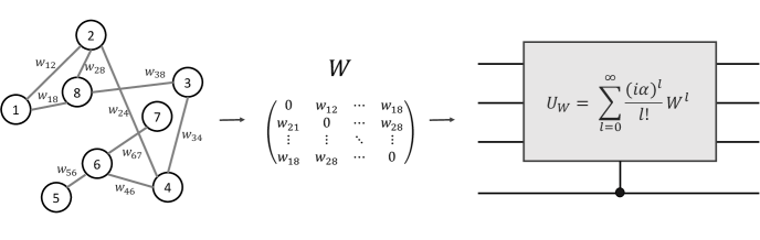
Our Approach: We propose a new variational quantum algorithm for approximately solving QSDPs that uses Hadamard Test objective functions and Approximate Amplitude Constraints (HTAAC-QSDP, Fig. 1).
Theorem 1
HTAAC-QSDP for the Goemans-Williamson algorithm uses qubits, a constant number of quantum measurements, and classical calculations to approximate SDPs with up to variables.
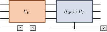
The details of the HTAAC-QSDP implementation must be engineered to each SDP and, in this work, we focus on the Goemans-Williamson algorithm [6], with particular emphasis on its application to MaxCut. In some cases, our method is nearly an exponential reduction in required expectation values, e.g., for high-constraint problems such as MaxCut. As described in Sec. 2, we achieve this, in part, through a unitary objective function encoding with the Hadamard Test [38] (Fig. 1(a)), which allows for the extremization of the entire -dimensional objective by estimating only a single quantum expectation value (Fig. 1(c)). Our quantum Goemans-Williamson algorimth for MaxCut requires amplitude constraints, which we effectively enforce with only 1) a constant number of quantum measurements from a second Hadamard Test (Fig. 1(b)) and 2) the estimation of a polynomial number of properly selected, commuting Pauli strings (Fig. 1(d)).
In Sec. 3, we demonstrate the success of the HTAAC-QSDP Goemans-Williamson algorithm (Algorithm 1) by approximating MaxCut [39] for large-scale graphs from the well-studied GSet graph library [40] (Fig. 5). In addition to satisfying the MaxCut approximation ratio [6], HTAAC-QSDP achieves cut values that are commensurate with the leading gradient-based classical SDP solvers [41], implying that we reach optima that are very near the global optimum of these SDP objective functions.
Finally, in Sec. 4.1 we discuss the feasibility of the Hadamard encoding. For general SDPs, we establish an upper bound (Theorem 2) on the phase of our Hadamard encoding, such that our technique is a high-quality approximation of the original SDP. The purpose of this upper bound is to demonstrate that tractably large values of the unitary phase are permissible (i.e., need not become arbitrarily small) for encoding a wide variety of large-scale problems. We discuss the known difficulty, and thus usefulness, of graph optimization problems under these conditions. Specifically:
Theorem 2
Our approximate Hadamard Test objective function (Sec. 2.1) holds for graphs with randomly distributed edges if
where is the number of non-zero edge weights and is the average number of edges per vertex.
We can view the criteria of Theorem 2 in two ways: for SDPs with arbitrarily many variables , the size of can be kept reasonably large while the Hadamard Test objective function (see Sec. 2.1) remains valid as long as 1) does not grow slower than the total number of edges , or 2) does not grow slower than the the cube of . Both of these conditions hold for graphs that are not too dense, meaning that they are widely satisfiable. For instance, the majority of interesting and demonstrably difficult graphs for MaxCut are relatively sparse [39, 10, 40, 42, 43]. We note that for graphs where edge-density is unevenly distributed, Theorem 2 should hold for the densest region of the graph, i.e., should be the average number of edges per vertex for the most highly connected vertices.
2 Efficient Quantum Semidefinite Programs
| (1) |
where is an symmetric matrix that encodes the optimization problem and () are symmetric matrices (scalars) that encode the problem constraints. denotes the trace inner product
| (2) |
In this section, we detail a method of efficient optimization of the above SDP objective and constraints using quantum methods (Fig. 1), specifically by implementing Hadamard Tests and imposing a polynomial number of Pauli constraints. We provide a concrete example in the form of the Goemans-Williamson [6] algorithm for MaxCut [39], as summarized in Algorithm 1.
2.1 The Hadamard Test as a Unitary Objective
In quantum analogy to the objective function of Eq. 1, we wish to minimize over the -qubit density matrices , which are positive semidefinite by definition. We generate these quantum ensembles from an initial density matrix such that , where is a variational quantum circuit. This yields the quantum objective function
| (3) |
Throughout most of this work, we consider pure states such that and , although we detail the case of mixed quantum states in Sec. 2.6. In the case of pure states, Eq. 3 yields
| (4) |
The Hadamard Test (Fig. 1(c)) is a quantum computing subroutine for arbitrary -qubit states and -qubit unitaries [38]. It allows the real or imaginary component of the -state inner product to be obtained by estimating only a single expectation value , which is the -axis Pauli spin on the th (auxiliary) qubit. For example, to obtain the imaginary component of , we prepare the quantum state and apply a controlled- from the th qubit to , followed by a Hadamard gate on the th qubit. This produces the state
| (5) |
upon which projective measurement yields
| (6) |
Rather than estimate the expectation values required to characterize and optimize the loss function of Eq. 3, our method encodes the -dimensional objective matrix as the imaginary part of an -qubit unitary (Fig. 1(a)). Here, the phase is a constant scalar. is then conditioned on the th (or auxilary) qubit as a controlled-unitary. We then use the Hadamard Test to calculate the objective term in the loss function
| (7) |
The intuition for this objective function is that, for sufficiently small , . By restricting ourselves to quantum circuits with real-valued output states, we render the single expectation value proportional to the objective function of Eq. 3, which requires expectation values to estimate. In Sec. 4.1, we analytically prove that, for many optimization problems, has a practical upper bound such that with a reasonably large , even for arbitrarily large .
2.2 Quantum Goemans-Williamson Algorithm
We now illustrate how can be a close approximation of , including for optimization problems with an arbitrarily large number of variables . For concreteness, we select the NP-complete problem MaxCut [39], and specifically focus on the corresponding NP-hard optimization problem [45]. This problem is of particular interest due to its favorable -approximation ratio with semidefinite programming techniques, notably the Goemans-Williamson algorithm [6], for which we now derive an efficient quantum implementation. The Goemans-Williamson algorithm is also applicable to to numerous other optimization problems, such as MaxSat and Max Directed Cut [6].
For a MaxCut problem with vertices , , let be the matrix that encodes the up to non-zero edge weights in its entries . As the vertices lack self-interaction, . The optimization problem is then defined as
| (8) |
which can be mapped to the classical SDP with constraints
| (9) |
| \topruleGraph | ||||
|---|---|---|---|---|
| G11 | ||||
| G12 | ||||
| G13 | ||||
| G14 | ||||
| G15 | ||||
| G20 | ||||
| G21 |
As described by Eq. 3, we can transform the optimization portion of Eq. 9 by substituting the classical positive semidefinite matrix for the quantum density operator . The solution to the SDP is then stored in , i.e., (for more details, see Sec. 2.3). As detailed in Sec. 2.1, the evaluation of this objective function can be optimized by estimating a single expectation value with the Hadamard Test. Likewise, we now introduce a quantum alternative to the constraint from Eq. 9. First, note that due to the orthonormality of quantum states, the exact quantum equivalent of Eq. 9 is
| (10) |
This rescaling changes neither the effectiveness nor the guarantees of the semidefinite program, because the salient feature of the constraint is that all of the quantum states have the same amplitude magnitude , such that all of the vertices are of equal magnitude and none are disproportionately favored. The solutions and differ only by a constant factor, such that . This yields the quantum MaxCut SDP
| (11) |
As graph weights are real-valued and symmetric (i.e., ), is Hermitian. We can thus use it as the generator of such that (Fig. 1(a))
| (12) |
As is real, the odd powers of in Eq. 12 are the imaginary components. The condition that is upheld iff, for the vast majority of variables , . Note that, when this condition holds, approximates with only vanishing error and a rescaling by . In Sec. 4.1, we prove Theorem 2, demonstrating that this condition is achievable with a tractable (i.e., larger than some fixed finite value that is constant in problem size ) for a wide variety of graphs.
Next, we note that enforcing the amplitude constraints would require the estimation of all -axis Pauli strings of order (all Pauli strings with Pauli- operators) of the state . This would be a total of expectation values. As an alternative to this large overhead, HTAAC-QSDP proposes the use of Approximate Amplitude Constraints (Fig. 1(d)). For example, consider the set of Pauli strings of length
| (13) |
where are the Pauli -operators on the th qubit. We can use these equalities as partial constraints for the -qubit output state . This set of constraints approximates the same restrictions as the set of constraints of Eq. 11 by limiting quantum correlations, as these indicate subsets of states with unequal populations. That is, each such -axis Pauli string is the difference of the total populations of two equal partitions of state space. To gain intuition, let us consider a two-qubit state and the Pauli string . Using the constraints for Eq. 13, we enforce the equality which, while not fully enforcing the constraints of Eq. 11 (e.g., not enforcing that all states have equal populations), does enforce equal populations among a subset of states. This results in a lighter-weight and more flexible set of constraints. As an example, promotes all state components to be populated by disallowing states where the first qubit is in a computational basis state, such as or . Likewise, the , -axis Pauli string constraint produces the equality , which would, for example, disallow the Bell State . We highlight that the Pauli string constraints of Eq. 13 are commuting, such that they can be estimated as different marginal distributions from a single set of -qubit -axis measurements.
We again emphasize that these constraints only approximately enforce the SDP constraint . Fully satisfying this constraint would require restricting Pauli- correlations between any subset of the qubits, such that no states of unequal amplitude magnitudes are permitted. Eq. 10 can be fully satisfied if we constrain with all of the Pauli strings of length . However, as there exist choose -axis Pauli strings of order , this requires estimating different expectation values and greatly decreases the efficiency of the algorithm. Sec. 3 details that, in practice for -vertex graphs, competitive results are obtained using only constraint terms (Fig. 2 and Table 2), and optimization performance is largely saturated with terms (Fig. 4 and Table 3).
In order to explicitly see how the constraints of Eq. 13 largely enforce the constraint , let us take the example of a three-qubit state (), which can encode up to eight vertices () using HTAAC-QSDP. Any real-valued state can be written generically as
and its constraints from Eq. 13 are
| (14) |
Combined with the normalization constraint , the above system of equations nearly guarantees that Eq. 10 is fulfilled. However, it still permits a small subset of states that do not satisfy Eq. 10 due to three-qubit correlations, e.g.,
States with higher-order correlations such as , which neither satisfy Eq. 10 nor are disallowed by Eq. 13, can be avoided by adding higher-order Pauli string constraints. For the above example, we would add the constraint , which would disallow as .
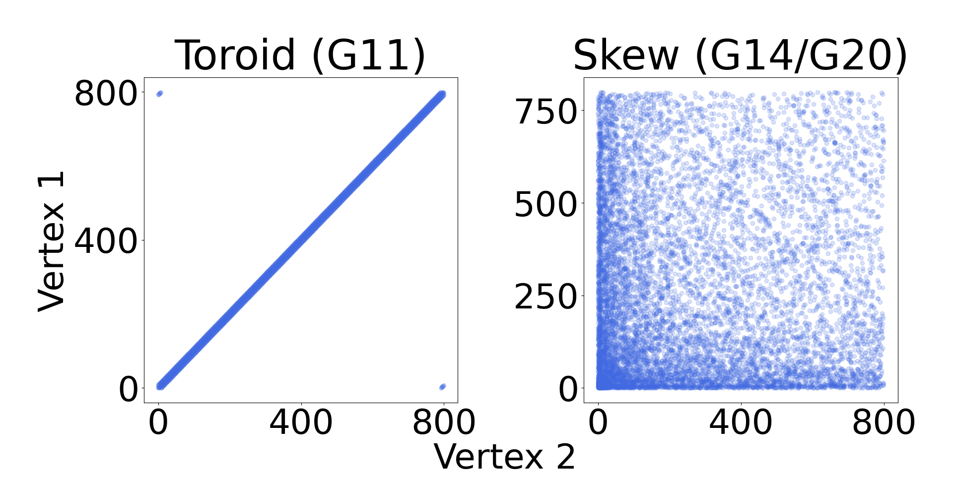
Eq. 10 can also be systematically undermined by the unequal distribution of graph edges among the quantum states. For instance, the asymmetrically distributed edge-weights in skewed graphs (Fig. 5 left and Sec. 3). With such graphs, the minimization of the loss function can lead to outsized state populations for quantum states that encode high-degree (high edge-weight) vertices. Moreover, as the number of classical variables will not generally be a power of two, there will often be quantum states that are not encoded with a classical variable. For example and as detailed in Sec. 3, we use qubits ( states) to optimize the -vertex () GSet graphs, such that the states to are absent from the objective function. In such cases, the minimization of the loss function can lead to outsized state populations of quantum states that are present in the optimization function. In principle, these imbalances can be addressed by increasing the magnitude of the Pauli string amplitude constraints, but this is known to cause poor objective function convergence [46].
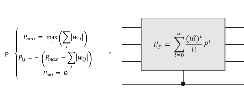
To redress this systematic skew, we add a population-balancing unitary (Fig. 1(b)), which is implemented on via a second Hadamard Test (Sec. 2.1, Fig. 1(c)) and adds the loss function term . Specifically, where is some diagonal operator of edge weights , where is an adjustable hyperparameter and is the maximum magnitude of edge weights for any given vertex. works to balance the state populations by premiating the occupation of states that are lesser represented by or absent from the objective function .
Combining both the efficient Hadamard Test objective function and the Approximate Amplitude Constraints, we can use simple gradient descent-based penalty methods [46] to find the solution. Specifically, we minimize the HTAAC-QSDP loss function for the Goemans-Williamson algorithm
| (15) |
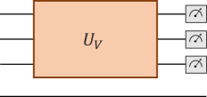
at each time step by preparing a quantum state on a variational quantum computer. The scalar is the penalty hyperparameter. While for simplicity we have chosen a single, time-constant for all constraints, in principle each constraint could be parameterized with a distinct , each of which could also vary as a function of . The number of quantum circuit preparations required to optimize our HTAAC-QSDP protocol is constant with respect to the number of qubits (and thus to the maximum number of vertices ), as and each require only the Pauli- measurement on the auxilary qubit, and the amplitude constraint terms can be calculated from a single set of -qubit measurements on the state . The classical complexity of each training step scales as just , as one marginal expectation value is calculated from the measurements for each of the constraints.
2.3 Retrieving SDP Solutions
At the end of our protocol, the SDP solution is encoded into . Like in other QSDP protocols, may either be used to extract the full -variable solution or for less computationally intensive analysis (i.e., to characterize the features of the solution or as an input state for further quantum protocols). For many SDPs, such as MaxCut, a good approximation of the solution (here, cut value) can also be extracted from the expectation values comprising the cost function.
To extract this approximate cut value, we note that Eq. 8 can be rewritten as
| (16) |
where . We note that this latter sum can be computed on a quantum device as
| (17) |
where is the Hadamard gate, as is the positive-phase and equal superposition of all states. Thus, can be estimated with a Hadamard test where is applied to the input state, which we here denote . Likewise, note that the second summation in Eq. 16 is given by
| (18) |
in the case that the constraints are well-enforced. This allows us to estimate the cut value with , the Hadamard test using the variationally prepared . Thus, the cost function can be estimated directly as
| (19) |
If the full solution is desired, then full real-space tomography of must be conducted by calculating the marginal distributions of all Pauli strings along the and -axes [47], although partial and approximate methods could make valuable contributions [48, 49]. We now show that once is determined, it suffices to assign the partition of each vertex as , or the sign of the state component .
In classical semidefinite programming algorithms, such as the Goemans-Williamson algorithm [6], the optimal solution is factorized by Cholesky decomposition into the product , where is an upper diagonal matrix. The sign of each vertex is then designated as
| (20) |
where are the column vectors of and is a length- vector of normally distributed random variables .
We define the quantum parallel by noting that as , its Cholesky decomposition is simply the matrix that has the first row and and all other entries equal to zero. In this decomposition, Eq. 20 reduces to
| (21) |
As MaxCut has symmetry, the cut values are symmetric under inversion, or flipping the sign of all vertices. This makes the sign of the normally distributed irrelevant to the graph partitioning. Without loss of generality, we can therefore set and classify each vertex as .
2.4 Error Convergence
We now demonstrate that our method has an approximately error convergence rate. Assuming that our loss function is a convex function, which is generally only locally and/or approximately satisfied, it has been established that it will converge as for iterations if it is -Lipschitz continuous [50].
While parameterized quantum circuits are known to be -Lipschitz continuous [24, 34], we here, in the name or thoroughness, explicitly demonstrate this for our particular loss function. Specifically, a function is -Lipschitz continuous if
| (22) |
for all parameter inputs and . will be -Lipschitz continuous if each of its components are independently so.
Starting with the objective function , note that
| (23) |
where is the generator of the unitary matrix parameterized by . Eq. 23 is now composed of two terms, each comprised entirely of normal matrices and vectors, save for perhaps the Hermitian generators , with some extremal eigenvalue . Then, and . This proof doubles for the constraint terms, save that we replace the unitary matrix with some Pauli string observable.
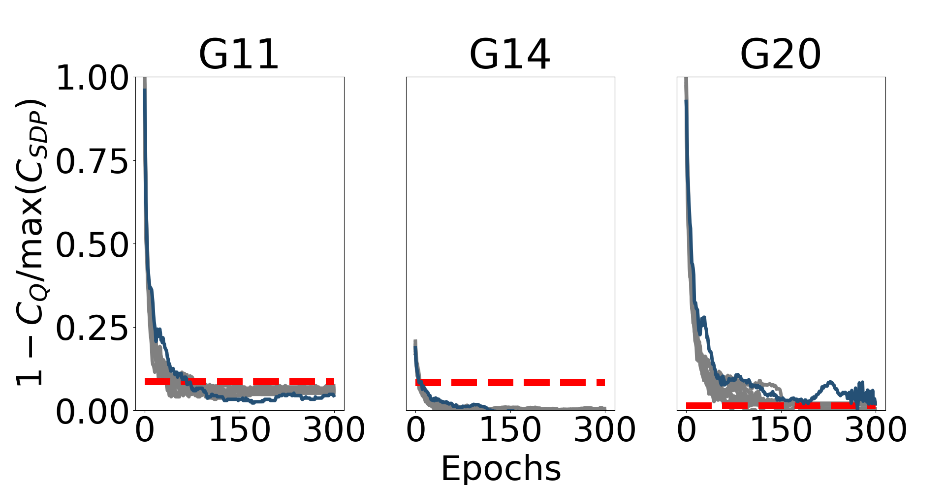
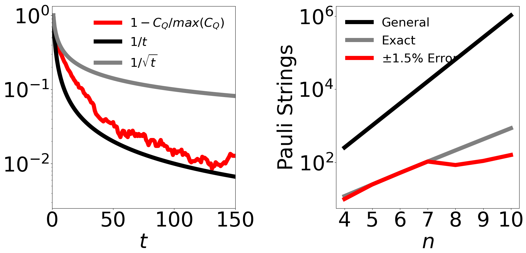
Fig. 6 (left) demonstrates this approximate convergence for the cut value of G11. The approximate nature of this convergence stems from both the discontinuous rounding process and the nonconvexities of the optimization space.
2.5 Extensions to Other SDPs
| \topruleGraph | ||||||
|---|---|---|---|---|---|---|
| G11 | () | () | () | () | () | |
| G14 | () | () | () | () | () | |
| G20 | () | () | () | () | () |
As explained above, the Goemans-Williamson algorithm [6] can be applied to numerous other optimization algorithms, such as MaxSat and Max Directed Cut [6]. Moreover, HTAAC-QSDP can be adapted to accommodate the constraints of various other SDPs. The use of our method is particularly advantageous when the constraints of a problem are amenable to being expressed through a tractable number of Pauli strings, or when these constraints can be approximately enforced by such a set of strings. The precise mapping of constraints to limited sets of Pauli strings depends on the problem at hand and may require some engineering. We here provide a few such examples.
2.5.1 Max and Min Bisection
As one example, consider the Min/Max Bisection problems [51]. Min/Max Bisection are particularly relevant to very-large-scale integration (VLSI) for integrated circuit design [52], a vital application area for large-scale SDPs.
The SDPs for estimating the Max Bisection problem has the standard form:
| (24) |
The first constraint is equivalent to requiring that half of the variables of be partitioned equally, hence the term “bisection”. In analogy with Eq. 11, Eq. 24 can be written as
| (25) |
The second of these two constraints can be enforced by the Pauli strings constraints of Eq. 13. For large and assuming no systematic correlations between the ordering of the vertices, the first constraint can be ensured by adding any single Pauli string constraint
| (26) |
where is any Pauli string of operators. To see how Eq. 26 enforces the first constraint of Eq. 11, consider that any operator induces a bit-flip on a subset of qubits, such that each state is mapped to another state . This means that is the sum of products , where for each , , as enforced by the Pauli-Z constraints of Eq. 13. If the probability that a random state of is positive is , then in the limit of large and uncorrelated vertex assignment
| (27) |
The above yields iff , which would correspond to the equal partitioning of the vertices required by the Bisection problems. In the case of correlated vertex encodings, the average of several Pauli- strings can be considered. We note that Eq. 26 can be modified to enforce any partition ratio by solving for (Eq. 27) with the desired .
2.5.2 MaxSat
MaxSat problems are another branch of optimization tasks with constraints that focus on equally weighted vertices. In Max -Sat problems, the number of logical boolean strings of length are maximized over a given set of boolean variables [53]. For example, Max -Sat is given by [6]
| (28) |
where and are the coefficients of the problem. To convert this problem into an SDP, we optimize the objective function
| (29) |
2.5.3 Correlation Matrix Calculation
Correlation matrices are key to a wide array of statistical applications and can be estimated with limited information using SDPs [54, 55]. In particular, autocorrelation dictates that correlation matrices have unit diagonals (), much like MaxCut, Min/Max Bisection, and MaxSat, and can thus be addressed with the rescaled quantum version (, Eq. 10) and approximated by the -axis Pauli string constraints. Meanwhile, the extremization of certain correlations (e.g., maximize/minimize ) and the enforcement of inequality and equality constraints (e.g., or ) can be enforced by additional constraints with either Pauli strings or the tomography of a select few state components.
2.6 HTAAC-QSDP with Mixed Quantum States
We now overview the implementation of the HTAAC-QSDP Goemans-Williamson algorithm with mixed quantum states, such as might occur on a noisy quantum device or by interacting the utilized qubits with a set of unmeasured qubits. While the formalism for measuring Pauli strings on such systems is well known, we demonstrate how the required Hadamard Test remains viable. We start with , some mixed state equivalent of the variational state . Upon application of the controlled- (without loss of generality for ) conditioned on the th qubit, we obtain the density matrix
| (30) |
Upon applying a Hadamard gate on the th qubit and measuring it along the -axis, we obtain
| (31) |
which is proportional to Eq. 3 with the same coefficient as prescribed by Eq. 7. This enables not only optimization, but also evaluation of the cut value estimation (Eq. 19), which is an accurate representation of the true cut value (Fig. 3). Alternatively, the element-wise rounded cut value calculated using Eq. 21 can still be utilized as an approximation to the traditional Goemans-Williamson rounding scheme. Although it would not result in the typical inner-product rounding, the sign of each vertex could still defined as the relative sign between each and .
This mixed state formalism of the HTAAC-QSDP Goemans-Williamson algorithm works not only in principle, but also in practice. Fig. 2 displays the best cut value of a mixed state formalism with otherwise equal parameters (dark blue). The mixed state was generated by adding an unmeasured qubit to the randomly parameterized quantum circuit, which was then traced over prior to minimization and cut classification. The higher rank states moderately improved the performance on most graphs, with a mean higher-rank SDP value of (G11), (G14), and (G20), compared to , , and in the rank-1 case.
3 Simulations and Results
The viability of our HTAAC-QSDP Goemans-Williamson algorithm is displayed in Fig. 2 and Table 2. We compare , the cut values obtained by HTAAC-QSDP, to , the best results obtained by the leading gradient-based classical method [41]. We study all of the -vertex MaxCut problems explored in [41] (Table 2) in order to make an extensive comparison with the leading classical gradient-based interior point method. These graphs represent a broad sampling from the well-studied GSet graph library [40]. Graphs G11, G12, and G13 have vertices that are connected to nearest-neighbors on a toroid structure and weights (Fig 5, right), while G14 and G15 (G20 and G21) have binary weights and (integer weights ) and randomly distributed edge density that is highly skewed towards the lower numbered vertices (Fig 5, left).
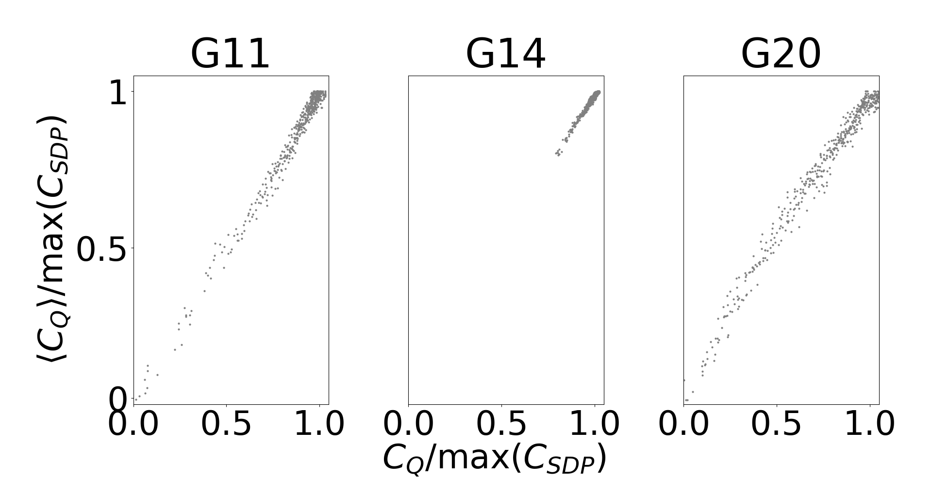
HTAAC-QSDP with -Pauli term constraints exceeds the performance of its classical counterpart on skewed binary and skewed integer graphs, and falls narrowly short of classical performance on toroid graphs (Fig. 2 and Table 2). The slight differences between the HTAAC-QSDP solution quality and those of the classical solver are typical of comparing different SDP solvers, which often differ slightly in their answers due to different numerical factors, including sparsity tolerance, rounding conventions (especially in the context of degenerate SDP solutions), and other hyperparameters [56]. All trajectories converge above the -approximation ratio (dashed red line) guaranteed by classical semidefinite programming, where is the highest known cut of each graph found by intensive, multi-shot, classical heuristics [44]. As SDPs are approximations of the optimization problem, the extremization of the loss function and the figure of merit (here, cut value) are highly correlated, particularly for well-enforced constraints. Fig. 3 demonstrates the strong correlation between the cut values estimated by quantum observables (Eq. 19) and the fully rounded SDP result , indicating that the HTAAC-QSDP Goemans-Williamson algorithm measurement of few quantum observables closely approximates the rounded and composited cut values of all variables.
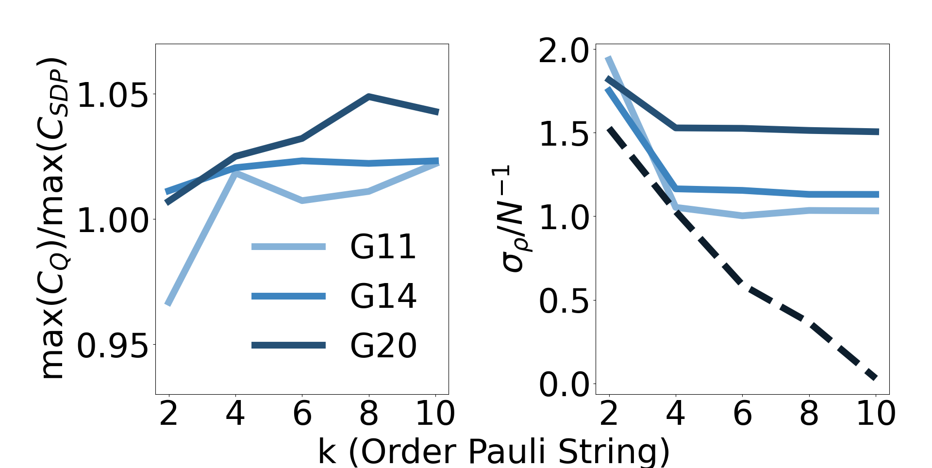
The addition of Pauli string amplitude constraints with can better enforce Eq. 10, leading to higher-quality solutions to the SDPs. Fig. 4 and Table 3 demonstrate that increasing produces moderately higher values for the -vertex graphs, until the performance increases saturate . Moreover, we note that at values , HTAAC-QSDP outperforms the analogous classical algorithm for all graph types, indicating a well-conditioned solution. Likewise, the population variance (solid lines) decreases substantially until saturating near at around .
Note that, in the absence of the competing objective function () dynamics, all Pauli- correlations become restricted as . This results in the complete constraint , such that (black dashed line in Fig. 4, left). We can understand this behavior in the context of other penalty methods [57]. In particular, consider the penalty methods formulation , where in our case are the time-dependent optimized parameters, , and represents the constraints. In the limits and , it is known that , where is the fully enforced solution of the hard constraints in some neighborhood of [58]. That is, the constraint-only dynamics (black dashed line of Fig. 4) represents the solution quality with respect to constraints in the limit.
The HTAAC-QSDP Goemans-Williamson algorithm was also tested against the G81 graph, a 20,000 vertex graph with a similar structure to G11-G13, and which is the largest MaxCut graph available that has been benchmarked against classical SDP methods. The average ratio between the HTAAC-QSDP obtained cut value for G81 and that of the classical counterpart was within of the -vertex toroid graphs tested (ratio of ). While the requisite circuit-depth for some quantum objective functions is known to grow linearly with the size of the circuit’s Hilbert space [59], this has not been shown for objective functions of the form of Eq. 15. This is in agreement with our observation that, while Hilbert space required to solve the G81 graphs is times larger than that for G11-G21, it’s circuit-depth is times larger. This reduction in requisite circuit-depth could also be due to the influence of constraints, which may effectively limit the degrees of freedom of the quantum circuit, a phenomenon that has been referred to as a “Hamiltonian informed” model [59].
That being said, even if the worst-case exponential bounds for quantum optimization were saturated, that would not preclude them from having lesser overhead than classical SDPs. We note that classically solving an NP-hard problem of variables is exponentially hard with respect to the variables (that is, it scales as ) and that, while these problems can be classically approximated using polynomial time and memory with respect to the number of variables, this still yields a classical complexity . For instance, the leading classical techniques, interior point methods [56], have a memory cost that scales as and a computational cost that scales as , making them in fact less efficient than the exponential bounds put on some worst-case quantum objective functions of memory cost and computational cost, a quartic and quadratic reduction, respectively.
Even among the lighter-weight yet often less powerful first-order methods, the classical overhead is considerable. For example, the popular branch of projection-based methods has arithmetic and memory complexity of and , respectively, for such variable problems [60]. Alternative algorithms, such as the Arora-Kale algorithm, can have time complexity as efficient as [61], although for problems such as MaxCut this still reduces to ). On a similar topic of scale, we note that G81 was optimized with constraints of orders , which results in a similar ratio of approximate to exact constraints as that of smaller experiments.
3.1 Simulation Details
All simulations are done using a one-dimensional ring qubit connectivity, such that each qubit has two neighbors and the th qubit neighbors the st qubit. The circuit ansatz of the simulations for graphs G11-G21 (G81) is () repetitions of two variationally parameterized -axis rotations interleaved with CNOT gates, alternating between odd-even and even-odd qubit control. The TensorLy-Quantum simulator [62, 63] is used for graphs G11-G21111Source code at https://github.com/tensorly/quantum/blob/main/doc/source/examples/htaacqsdp.py., while a modified version of cuStateVec [64] is used for G81. Gradient descent was conducted an ADAM [65] optimizer, with learning rate () for graphs G11-G21 (G81), as well as hyperparameters , and .
The evolution angle was set as for all graphs. The values of used in this work were for the toroid graphs and for the skew binary and skew integer graphs. We did not employ a unitary for the G81 graph. values should be chosen such that , as diagonal entries are always satisfiable (i.e., some population can always be placed on the state, lowering the loss function), in contrast to edge cuts, which are not (i.e., not every edge can be cut with any given partition for general graphs). values can be tuned on the device in the real time by monitoring the Pauli string constraints and choosing a that leads to largely satisfied Pauli constraints with relatively small coefficients , such that the convergence of the algorithm is not hindered by large constraints that outweigh the objective function or lead to unstable convergence. In this work, we set , to keep the total influence of constraint terms in proportion to the objective term . Specifically, for the -vertex graphs, we choose for the toroid and skew binary graphs and for the skew integer graphs. For the G81 graph, .
4 Theoretical Analysis of Hadamard Test Unitaries
This subsection addresses the implementation of the Hadamard tests found in this work, including the approximation of by with a finite phase , the construction of for difficult problems, and the implementation of the prescribed Hadamard Tests using ZX-calculus.
4.1 Finite Phase for Unitary Objective Function
In this subsection, we derive Theorem LABEL:theorem.general_claims, which we here restate for completeness:
Theorem 1 Our approximate Hadamard Test objective function (Sec. 2.1) holds for graphs with randomly distributed edges if
where is the number of non-zero edge weights and is the average number of edges per vertex.
As discussed above, Theorem 2 can be understood in two ways: that satisfies the approximation of Eq. 32 while remaining tractably large for SDPs of arbitrary , as long as does not 1) grow slower than the total number of edges , or 2) grow slower than the the cube of . We again note that Theorem 2 should hold for the densest graph region if the edge density is assymetrically distributed, i.e., should be the average number of edges for the densest vertices. As the conditions of Theorem 2 hold for graphs that are not too dense, they are widely satisfiable as the majority of interesting and demonstrably difficult graphs for MaxCut are relatively sparse [39, 10, 40, 42, 43]. Many classes of graphs for which MaxCut is NP-hard satisfy Theorem 2 with tractably large , even for arbitrarily large .
As an example, we consider non-planar graphs, for which optimization problems like MaxCut are typically NP-complete. While planar graphs can be solved in polynomial time [66], a graph is guaranteeably non-planar when , which reduces to in the limit of large [67]222Other families of easy graphs are even more restrictive, such as graphs that lack a giant component. In the limit of large , these graphs only occur in more than a negligible fraction of all possible graphs when and thus [68].. In accordance with Theorem 2, constant values of actually permit to grow as , while for constant can grow as , such that our approximation is valid for a wide variety of large-scale non-planar graphs. Indeed, most standard benchmarking graph sets have a small average number of edges per vertex, e.g., [40, 42, 43], as sparse edge-density is common among graphs with real-world applications. In fact, solving MaxCut with many classes of dense graphs (i.e., graphs with nearly all non-zero edges) is provably less challenging, and therefore less interesting, than with their relatively sparse counterparts [69].
We here sketch a brief proof of Theorem 2 for Erdös–Rényi random graphs [70] with edge weights , where is the uniform distribution on the interval . The edge density of a graph is described as , where is the number of non-zero edges and is the number of total possible edges. We provide a detailed proof of this and other graph types in the Appendix A.
Proof sketch of Theorem 2:
-
•
The Hadamard Test encoding is a good approximation when .
-
•
This is satisfied when for typical edges between vertices ,.
-
•
The mean of the non-zero elements in is 333The mean value of all elements of is , however the relevant comparison is between the elements of and the non-zero elements of ..
-
•
Elements are the sum of terms , with expectation value . That is, the additive error between the Hadamard encoding terms and the matrix elements scales as .
-
•
.
-
•
Substituting and , we obtain Theorem 2.
4.2 Construction of
While some optimization problems of variables may only be represented by graphs of distinct Pauli strings, we here illustrate that there are many interesting (indeed, NP-hard optimization problems) for which this is not the case. In particular, we focus on the MaxCut problem and discuss toroid and Erdos Renyi random graphs.
Toroid graphs, or graphs that can be embedded on a toroid such that none of the edges connecting vertices cross, have a regular, yet still three-dimensional (non-planar), topological structure [71]. While encoding difficult problems, these data sets can often be represented in just Pauli strings, as is the case with the 8-100 tourus family to which G11 pertains (Fig. 6, right, gray). What is more, the number of Pauli strings can be reduced even further by instead constructing an approximate operator and permitting a small amount of error (Fig. 6, right, red). The population balancing graphs are a similar subset of structured graphs, whose diagonality renders them expressible with Pauli strings of only -axis and identity gates.
Likewise, we can use similarly few terms to construct Erdös–Rényi random graphs, in which edges between any two vertices are equally likely and occur with probability [70]. As Pauli strings are a spanning set, these same statistics are replicated when such strings are chosen randomly. Moreover, we note that each Pauli string adds edges, such that the graph is rapidly populated.
4.3 Construction of Controlled Unitaries
The construction of unitary rotations and follows naturally from ZX calculus [72]. Specifically, Pauli Gadgets can be used to generalize unitary rotations from the qubit to which they are applied to multiple qubits through the use of CNOT gates, one on either size of each qubit and its rotated counterparts in a conjugated ladder scheme [73]. Moreover, rotations along distinct Pauli axes are achieved by conjugating these qubits with rotation gates along said axis. The gates are selected to match the terms of or and is the phase applied.
As this method generalizes to all rotations, it can also be paired with the controlled gates required for the Hadamard Test. Specifically, the Pauli rotation gate applied to the auxiliary-adjacent qubit is fashioned as a controlled rotation, with the control conditioned on the auxiliary qubit. Moreover, the small values of used in this work make the addition of multiple Pauli terms by Trotterization favorable, as the error of this technique is bounded by times the spectral norm [74].
5 Conclusion
The efficient optimization of very large-scale SDPs on variational quantum devices has to the potential to revolutionize their use in operations, computer architecture, and networking applications. In this manuscript, we have introduced HTAAC-QSDP, which uses qubits to approximate SDPs of up to variables and constraints by taking only a constant number of quantum measurements and a polynomial number of classical calculations per epoch. As we approximately encode the SDP objective function into a unitary operator, the Hadamard Test can be used to optimize arbitrarily large SDPs by estimating a constant number of expectation values. Likewise, we demonstrate that the constraints of many SDPs can also be efficiently enforced with approximate amplitude constraints.
Devising a quantum implementation of the Goemans-Williamson algorithm, we approximately enforce the constraints with a population-balancing Hadamard Test and the estimation of as few as Pauli string expectation values. We demonstrate our method on a wide array of graphs from the GSet library [40], approaching and often exceeding the performance of the leading gradient-based classical SDP solver on all graphs [41]. Finally, we note that by increasing the order of our Pauli string constraints, we improve the accuracy of our results, exceeding the classical performance on all graphs while still estimating only polynomially-many expectation values.
The approximate amplitude constraints of HTAAC-QSDP make it particularly helpful for problems with a large number of constraints . The benefits of using the Hadamard Test objective function depend on the original optimization problem. The optimization matrix of many NP-hard problems can be encoded with controlled-unitaries of polynomially-many Pauli terms, such that the Hadamard Test would be efficient to implement. While such cases could instead be optimized by directly estimating polynomially-many different non-commuting expectation values, use of the Hadamard Test circumvents the need to prepare an ensemble of output states for each Pauli term, eliminating these extra circuit preparations. Conversely, optimizing worst-case objective functions with the Hadamard Test would require controlled-unitaries with up to Pauli terms. While exact implementation of these problems with HTAAC-QSDP on purely gate-based quantum computers would be inefficient, such objective functions could be engineered as the natural time-evolution of quantum devices with rich interactions (e.g., quantum simulators [75, 76, 77] in their future iterations), or by approximate means.
Due to the immense importance of SDPs in scientific and industrial optimization, as well as the ongoing efforts to generate effective quantum SDP methods that are often limited by poor scaling in key parameters such as accuracy and problem size, our work provides a variational alternative with tractable overhead. In particular, the largest SDPs solved via classical methods, which required over 500 teraFLOPs on nearly ten-thousand CPUs and GPUs [78], could be addressed by our method with just qubits.
In future work, the techniques of this manuscript can be extended to additional families of SDPs. For instance, SDPs that extremize operator eigenvalues are a natural application for quantum circuits [79]. Similarly, variational quantum linear algebra techniques [80] can potentially be adapted to enforce the more general constraints
of Eq. 1. In many cases, more general constraints are likewise satisfiable with the Pauli string constraints, as suggested in this work. For instance, when the number of requisite constraints is much smaller than the number of variables , or, as is the case with our quantum implementation of the Goemans-Williamson algorithm, by enforcing a relatively small subset of the constraints.
6 Acknowledgments
At CalTech, A.A. is supported in part by the Bren endowed chair, and Microsoft, Google, Adobe faculty fellowships. S.F.Y. thanks the AFOSR and the NSF (through the CUA PFC and QSense QLCI) for funding. The authors would like to thank Matthew Jones, Robin Alexandra Brown, Eleanor Crane, Alexander Schuckert, Madelyn Cain, Austin Li, Omar Shehab, Antonio Mezzacapo, Mark M. Wilde, and Patrick J. Coles for useful conversations.
References
- [1] Stephen P. Boyd and Lieven Vandenberghe. “Convex optimization”. Cambridge Press. (2004).
- [2] Michel X. Goemans. “Semidefinite programming in combinatorial optimization”. Mathematical Programming 79, 143–161 (1997).
- [3] Lieven Vandenberghe and Stephen Boyd. “Applications of semidefinite programming”. Applied Numerical Mathematics 29, 283–299 (1999).
- [4] Wenjun Li, Yang Ding, Yongjie Yang, R. Simon Sherratt, Jong Hyuk Park, and Jin Wang. “Parameterized algorithms of fundamental np-hard problems: a survey”. Human-centric Computing and Information Sciences 10, 29 (2020).
- [5] Christoph Helmberg. “Semidefinite programming for combinatorial optimization”. Konrad-Zuse-Zentrum fur Informationstechnik Berlin. (2000).
- [6] Michel X. Goemans and David P. Williamson. “Improved approximation algorithms for maximum cut and satisfiability problems using semidefinite programming”. J. ACM 42, 1115–1145 (1995).
- [7] Florian A. Potra and Stephen J. Wright. “Interior-point methods”. Journal of Computational and Applied Mathematics 124, 281–302 (2000).
- [8] Haotian Jiang, Tarun Kathuria, Yin Tat Lee, Swati Padmanabhan, and Zhao Song. “A faster interior point method for semidefinite programming”. In 2020 IEEE 61st annual symposium on foundations of computer science (FOCS). Pages 910–918. IEEE (2020).
- [9] Baihe Huang, Shunhua Jiang, Zhao Song, Runzhou Tao, and Ruizhe Zhang. “Solving sdp faster: A robust ipm framework and efficient implementation”. In 2022 IEEE 63rd Annual Symposium on Foundations of Computer Science (FOCS). Pages 233–244. IEEE (2022).
- [10] David P. Williamson and David B. Shmoys. “The design of approximation algorithms”. Cambridge University Press. (2011).
- [11] Nikolaj Moll, Panagiotis Barkoutsos, Lev S Bishop, Jerry M Chow, Andrew Cross, Daniel J Egger, Stefan Filipp, Andreas Fuhrer, Jay M Gambetta, Marc Ganzhorn, et al. “Quantum optimization using variational algorithms on near-term quantum devices”. Quantum Science and Technology 3, 030503 (2018).
- [12] Edward Farhi, Jeffrey Goldstone, Sam Gutmann, and Michael Sipser. “Quantum computation by adiabatic evolution” (2000). arXiv:quant-ph/0001106.
- [13] Tameem Albash and Daniel A. Lidar. “Adiabatic quantum computation”. Rev. Mod. Phys. 90, 015002 (2018).
- [14] Sepehr Ebadi, Alexander Keesling, Madelyn Cain, Tout T Wang, Harry Levine, Dolev Bluvstein, Giulia Semeghini, Ahmed Omran, J-G Liu, Rhine Samajdar, et al. “Quantum optimization of maximum independent set using rydberg atom arrays”. Science 376, 1209–1215 (2022).
- [15] Tadashi Kadowaki and Hidetoshi Nishimori. “Quantum annealing in the transverse ising model”. Phys. Rev. E 58, 5355–5363 (1998).
- [16] Elizabeth Gibney. “D-wave upgrade: How scientists are using the world’s most controversial quantum computer”. Nature541 (2017).
- [17] Edward Farhi, Jeffrey Goldstone, and Sam Gutmann. “A quantum approximate optimization algorithm”. arXiv (2014). arXiv:1411.4028.
- [18] Juan M Arrazola, Ville Bergholm, Kamil Brádler, Thomas R Bromley, Matt J Collins, Ish Dhand, Alberto Fumagalli, Thomas Gerrits, Andrey Goussev, Lukas G Helt, et al. “Quantum circuits with many photons on a programmable nanophotonic chip”. Nature 591, 54–60 (2021).
- [19] Fernando G. S. L. Brandão, Amir Kalev, Tongyang Li, Cedric Yen-Yu Lin, Krysta M. Svore, and Xiaodi Wu. “Quantum SDP Solvers: Large Speed-Ups, Optimality, and Applications to Quantum Learning”. 46th International Colloquium on Automata, Languages, and Programming (ICALP 2019) 132, 27:1–27:14 (2019).
- [20] Joran Van Apeldoorn and András Gilyén. “Improvements in quantum sdp-solving with applications”. In Proceedings of the 46th International Colloquium on Automata, Languages, and Programming (2019).
- [21] Joran van Apeldoorn, Andràs Gilyèn, Sander Gribling, and Ronald de Wolf. “Quantum sdp-solvers: Better upper and lower bounds”. Quantum 4, 230 (2020).
- [22] Fernando G.S.L. Brandão and Krysta M. Svore. “Quantum speed-ups for solving semidefinite programs”. In 2017 IEEE 58th Annual Symposium on Foundations of Computer Science (FOCS). Pages 415–426. (2017).
- [23] Fernando G.S L. Brandão, Richard Kueng, and Daniel Stilck França. “Faster quantum and classical SDP approximations for quadratic binary optimization”. Quantum 6, 625 (2022).
- [24] Dhrumil Patel, Patrick J. Coles, and Mark M. Wilde. “Variational quantum algorithms for semidefinite programming” (2021). arXiv:2112.08859.
- [25] Anirban N. Chowdhury, Guang Hao Low, and Nathan Wiebe. “A variational quantum algorithm for preparing quantum gibbs states” (2020). arXiv:2002.00055.
- [26] Taylor L Patti, Omar Shehab, Khadijeh Najafi, and Susanne F Yelin. “Markov chain monte carlo enhanced variational quantum algorithms”. Quantum Science and Technology 8, 015019 (2022).
- [27] Youle Wang, Guangxi Li, and Xin Wang. “Variational quantum gibbs state preparation with a truncated taylor series”. Physical Review Applied 16, 054035 (2021).
- [28] Sanjeev Arora, Elad Hazan, and Satyen Kale. “The multiplicative weights update method: A meta-algorithm and applications”. Theory of Computing 8, 121–164 (2012).
- [29] Iordanis Kerenidis and Anupam Prakash. “A quantum interior point method for lps and sdps”. ACM Transactions on Quantum Computing1 (2020).
- [30] Brandon Augustino, Giacomo Nannicini, Tamás Terlaky, and Luis F. Zuluaga. “Quantum interior point methods for semidefinite optimization” (2022). arXiv:2112.06025.
- [31] M. Cerezo, Andrew Arrasmith, Ryan Babbush, Simon C. Benjamin, Suguru Endo, Keisuke Fujii, Jarrod R. McClean, Kosuke Mitarai, Xiao Yuan, Lukasz Cincio, and Patrick J. Coles. “Variational quantum algorithms”. Nature Reviews Physics 3, 625–644 (2021).
- [32] Kishor Bharti, Tobias Haug, Vlatko Vedral, and Leong-Chuan Kwek. “Noisy intermediate-scale quantum algorithm for semidefinite programming”. Phys. Rev. A 105, 052445 (2022).
- [33] Lennart Bittel and Martin Kliesch. “Training variational quantum algorithms is np-hard”. Phys. Rev. Lett. 127, 120502 (2021).
- [34] Jarrod R. McClean, Sergio Boixo, Vadim N. Smelyanskiy, Ryan Babbush, and Hartmut Neven. “Barren plateaus in quantum neural network training landscapes”. Nature Communications 9, 4812 (2018).
- [35] Carlos Ortiz Marrero, Mária Kieferová, and Nathan Wiebe. “Entanglement-induced barren plateaus”. PRX Quantum 2, 040316 (2021).
- [36] Taylor L. Patti, Khadijeh Najafi, Xun Gao, and Susanne F. Yelin. “Entanglement devised barren plateau mitigation”. Phys. Rev. Res. 3, 033090 (2021).
- [37] Arthur Pesah, M. Cerezo, Samson Wang, Tyler Volkoff, Andrew T. Sornborger, and Patrick J. Coles. “Absence of barren plateaus in quantum convolutional neural networks”. Phys. Rev. X 11, 041011 (2021).
- [38] Dorit Aharonov, Vaughan Jones, and Zeph Landau. “A polynomial quantum algorithm for approximating the jones polynomial”. Algorithmica 55, 395–421 (2009).
- [39] Clayton W. Commander. “Maximum cut problem, max-cutmaximum cut problem, max-cut”. Pages 1991–1999. Springer US. Boston, MA (2009).
- [40] Steven J. Benson, Yinyu Yeb, and Xiong Zhang. “Mixed linear and semidefinite programming for combinatorial and quadratic optimization”. Optimization Methods and Software 11, 515–544 (1999).
- [41] Changhui Choi and Yinyu Ye. “Solving sparse semidefinite programs using the dual scaling algorithm with an iterative solver”. Manuscript, Department of Management Sciences, University of Iowa, Iowa City, IA52242 (2000). url: web.stanford.edu/ yyye/yyye/cgsdp1.pdf.
- [42] Angelika Wiegele. “Biq mac library – a collection of max-cut and quadratic 0-1 programming instances of medium size”. Alpen-Adria-Universität Klagenfurt (2007). url: biqmac.aau.at/biqmaclib.pdf.
- [43] Stefan H. Schmieta. “The dimacs library of mixed semidefinite-quadratic-linear programs”. 7th DIMACS Implementation Challenge (2007). url: http://archive.dimacs.rutgers.edu.
- [44] Yoshiki Matsuda. “Benchmarking the max-cut problem on the simulated bifurcation machine”. Medium (2019). url: medium.com/toshiba-sbm/benchmarking-the-max-cut-problem-on-the-simulated-bifurcation-machine-e26e1127c0b0.
- [45] R. M. Karp. “Reducibility among combinatorial problems”. Springer US. Boston, MA (1972).
- [46] Dimitri P Bertsekas. “Constrained optimization and lagrange multiplier methods”. Academic press. (1982).
- [47] G Mauro D’Ariano, Matteo GA Paris, and Massimiliano F Sacchi. “Quantum tomography”. Advances in imaging and electron physics 128, 206–309 (2003).
- [48] Alessandro Bisio, Giulio Chiribella, Giacomo Mauro D’Ariano, Stefano Facchini, and Paolo Perinotti. “Optimal quantum tomography”. IEEE Journal of Selected Topics in Quantum Electronics 15, 1646–1660 (2009).
- [49] Max S. Kaznady and Daniel F. V. James. “Numerical strategies for quantum tomography: Alternatives to full optimization”. Phys. Rev. A 79, 022109 (2009).
- [50] Javier Peña. “Convergence of first-order methods via the convex conjugate”. Operations Research Letters 45, 561–564 (2017).
- [51] Alan Frieze and Mark Jerrum. “Improved approximation algorithms for maxk-cut and max bisection”. Algorithmica 18, 67–81 (1997).
- [52] Clark David Thompson. “A complexity theory for vlsi”. PhD thesis. Carnegie Mellon University. (1980). url: dl.acm.org/doi/10.5555/909758.
- [53] Chu Min Li and Felip Manya. “Maxsat, hard and soft constraints”. In Handbook of satisfiability. Pages 903–927. IOS Press (2021).
- [54] Nicholas J Higham. “Computing the nearest correlation matrix—a problem from finance”. IMA journal of Numerical Analysis 22, 329–343 (2002).
- [55] Tadayoshi Fushiki. “Estimation of positive semidefinite correlation matrices by using convex quadratic semidefinite programming”. Neural Computation 21, 2028–2048 (2009).
- [56] Todd MJ. “A study of search directions in primal-dual interior-point methods for semidefinite programming”. Optimization methods and software 11, 1–46 (1999).
- [57] Roger Fletcher. “Penalty functions”. Mathematical Programming The State of the Art: Bonn 1982Pages 87–114 (1983).
- [58] Robert M Freund. “Penalty and barrier methods for constrained optimization”. Lecture Notes, Massachusetts Institute of Technology (2004). url: ocw.mit.edu/courses/15-084j-nonlinear-programming-spring-2004.
- [59] Eric Ricardo Anschuetz. “Critical points in quantum generative models”. In International Conference on Learning Representations. (2022). url: openreview.net/forum?id=2f1z55GVQN.
- [60] Amir Beck. “First-order methods in optimization”. SIAM. (2017).
- [61] Sanjeev Arora and Satyen Kale. “A combinatorial, primal-dual approach to semidefinite programs”. J. ACM63 (2016).
- [62] Taylor L. Patti, Jean Kossaifi, Susanne F. Yelin, and Anima Anandkumar. “Tensorly-quantum: Quantum machine learning with tensor methods” (2021). arXiv:2112.10239.
- [63] Jean Kossaifi, Yannis Panagakis, Anima Anandkumar, and Maja Pantic. “Tensorly: Tensor learning in python”. Journal of Machine Learning Research 20, 1–6 (2019). url: http://jmlr.org/papers/v20/18-277.html.
- [64] cuQuantum Team. “Nvidia/cuquantum: cuquantum v22.11” (2022).
- [65] Diederik P. Kingma and Jimmy Ba. “Adam: A method for stochastic optimization” (2017). arXiv:1412.6980.
- [66] Brahim Chaourar. “A linear time algorithm for a variant of the max cut problem in series parallel graphs”. Advances in Operations Research (2017).
- [67] Yury Makarychev. “A short proof of kuratowski’s graph planarity criterion”. Journal of Graph Theory 25, 129–131 (1997).
- [68] Béla Bollobás. “The evolution of random graphs—the giant component”. Page 130–159. Cambridge Studies in Advanced Mathematics. Cambridge University Press. (2001). 2 edition.
- [69] Sanjeev Arora, David Karger, and Marek Karpinski. “Polynomial time approximation schemes for dense instances of np-hard problems”. Journal of computer and system sciences 58, 193–210 (1999).
- [70] Rick Durrett. “Erdös–rényi random graphs”. Page 27–69. Cambridge Series in Statistical and Probabilistic Mathematics. Cambridge University Press. (2006).
- [71] Gary Chartrand and Ping Zhang. “Chromatic graph theory”. Taylor and Francis. (2008).
- [72] John van de Wetering. “Zx-calculus for the working quantum computer scientist” (2020). arXiv:2012.13966.
- [73] Alexander Cowtan, Silas Dilkes, Ross Duncan, Will Simmons, and Seyon Sivarajah. “Phase gadget synthesis for shallow circuits”. Electronic Proceedings in Theoretical Computer Science 318, 213–228 (2020).
- [74] Andrew M. Childs, Yuan Su, Minh C. Tran, Nathan Wiebe, and Shuchen Zhu. “Theory of trotter error with commutator scaling”. Phys. Rev. X 11, 011020 (2021).
- [75] Joseph W Britton, Brian C Sawyer, Adam C Keith, C-C Joseph Wang, James K Freericks, Hermann Uys, Michael J Biercuk, and John J Bollinger. “Engineered two-dimensional ising interactions in a trapped-ion quantum simulator with hundreds of spins”. Nature 484, 489–492 (2012).
- [76] Hannes Bernien, Sylvain Schwartz, Alexander Keesling, Harry Levine, Ahmed Omran, Hannes Pichler, Soonwon Choi, Alexander S Zibrov, Manuel Endres, Markus Greiner, et al. “Probing many-body dynamics on a 51-atom quantum simulator”. Nature 551, 579–584 (2017).
- [77] Gheorghe-Sorin Paraoanu. “Recent progress in quantum simulation using superconducting circuits”. Journal of Low Temperature Physics 175, 633–654 (2014).
- [78] Katsuki Fujisawa, Hitoshi Sato, Satoshi Matsuoka, Toshio Endo, Makoto Yamashita, and Maho Nakata. “High-performance general solver for extremely large-scale semidefinite programming problems”. In SC ’12: Proceedings of the International Conference on High Performance Computing, Networking, Storage and Analysis. Pages 1–11. (2012).
- [79] Adrian S. Lewis and Michael L. Overton. “Eigenvalue optimization”. Acta Numerica 5, 149–190 (1996).
- [80] Xiaosi Xu, Jinzhao Sun, Suguru Endo, Ying Li, Simon C. Benjamin, and Xiao Yuan. “Variational algorithms for linear algebra”. Science Bulletin 66, 2181–2188 (2021).
Appendix A Appendix: Theoretical Analysis of Hadamard Test Objective Function
We now derive Theorem 2 in detail. In order for the efficient encoding to hold, it is sufficient to enforce that the third-order term in Eq. 12 is substantially smaller than the first-order term. That is
| (32) |
for typical edges between vertices ,. By induction, the criterion in Eq. 32 also guarantees that odd (imaginary) powers will likewise be smaller than the first order term, and are thus also negligible. While this condition can always be satisfied with an arbitrarily small , we in practice require that maintain some finite size to avoid unitary rotations with vanishingly small gate times and imaginary components . We now demonstrate that this criteria can be met for a wide array of graphs with NP-complete MaxCut optimization complexity.
First, we consider Erdös–Rényi random graphs [70] with elements , which are uniformly distributed on the interval . The graphs are said to have edge density , which is the fraction of non-zero edges over total possible edges . Typical elements are the sum of terms , with expectation value , such that the matrix elements of have the expectation value . As the mean of the non-zero elements in is , the criterion of Eq. 32 becomes
| (33) |
We can rewrite this criterion in terms the number of non-zero edges by noting that graph density scales as , where is the number of non-zero edges possible for an vertex graph. Likewise, the average number of edges per vertex is then , and Eq. 33 can be rewritten as
| (34) |
For graphs where edge density is not uniformly distributed, the above conditions should hold for the most densely connected vertices of the graph.
We briefly illustrate how our approximation holds for a few other classes of graphs. For instance, graphs with elements drawn from uniform distributions with both positive and negative components generally require ranges that are even more permissible (i.e., can be even larger) than those of the positive case, with the criterion of Eq. 33 serving as a small lower-bound.
Similar proofs of implementability can also be done for graphs with normally distributed weights of mean and variance . For the case , and need only satisfy
| (35) |