Quantum gradient descent algorithms for nonequilibrium steady states and linear algebraic systems
Abstract
The gradient descent approach is the key ingredient in variational quantum algorithms and machine learning tasks, which is an optimization algorithm for finding a local minimum of an objective function. The quantum versions of gradient descent have been investigated and implemented in calculating molecular ground states and optimizing polynomial functions. Based on the quantum gradient descent algorithm and Choi-Jamiolkowski isomorphism, we present approaches to simulate efficiently the nonequilibrium steady states of Markovian open quantum many-body systems. Two strategies are developed to evaluate the expectation values of physical observables on the nonequilibrium steady states. Moreover, we adapt the quantum gradient descent algorithm to solve linear algebra problems including linear systems of equations and matrix-vector multiplications, by converting these algebraic problems into the simulations of closed quantum systems with well-defined Hamiltonians. Detailed examples are given to test numerically the effectiveness of the proposed algorithms for the dissipative quantum transverse Ising models and matrix-vector multiplications.
PACS number(s): 02.30.Mv, 02.60.Pn, 03.67.Lx, 03.65.Yz
Keywords: Quantum simulation, Quantum gradient descent algorithm, Nonequilibrium steady state, Quantum open system
I Introduction
Quantum computers can effectively simulate the dynamics of quantum systems Feynman1982Simulating ; Bacon2010Recent ; Childs2012Hamiltonian , prepare quantum states Xin2019Preparation ; Yang2019Dissipative and solve machine learning tasks Shor1994 ; Grover1996 ; HHL2009 ; QML2017 ; Li2020Efficient ; Ye2021Generic ; Ran2020Tensor , although the related algorithms generally require deep gate sequences. In the past years, rapid advances in the construction of large-scale fault-tolerate universal quantum computers have been made based on, for instance, superconducting qubits Krantz2019A ; Huang2020Superconducting ; Wu2021Strong , photos Slussarenkoa2019Photonic , silicon quantum dots Yang2019Silicon and ultracold trapped ions Blatt2012Quantum ; Bruzewicza2019Trapped .
Currently, we are in an era of noisy intermediate-scale quantum (NISQ) processors that may have limited resources such as a few tens to hundreds of qubits with no error correction capability, shallow circuit depth and short coherence time preskill2018quantum ; larose2019variational ; peruzzo2014variational ; higgott2019variational ; jones2019variational . Such devices have ushered in the era of variational quantum algorithms (VQAs). VQAs aim to tackle complex problems by combining classical computers and NISQ devices benedetti2019parameterized ; wang2020variational ; li2021optimizing ; Liu2021Hybrid ; Liang2021Quantum. Experimental evidence related to VQAs suggests that NISQ devices may improve machine learning performance for image generation Huang2021Experimental , classification havlivcek2019supervised and combinatorial optimization problems Harrigan2021Quantum .
Different from VQAs, the full quantum eigensolver (FQE) finds the ground state of a hermitian Hamiltonian of a closed quantum system wei2020a ; Long2006General on a quantum computer without classical optimizers. In particular, due to the fact that the iterative optimization part utilizes the quantum gradient descent (QGD) algorithm, FQE does not require quantum-classical optimization loops like VQAs and thus can be applied totally on a quantum computer. This significant example implies that QGD as an optimization scheme is of importance in the NISQ era Fan2021Exponential .
Inspired by FQE for chemistry simulation, here we try to find interesting applications of QGD in open quantum systems and linear algebraic systems. In reality, the coupling to the environment is unavoidable for quantum systems and may lead to a rich variety of novel physical phenomena diehl2008quantum ; verstraete2009quantum . When the interaction with the environment is a Markovian one, the open quantum system is governed by the quantum master equation in the Lindblad form breuer2002the ; rotter2009a . As a result, the dynamics of the system give rise to incoherent characteristics such as damping and dephasing process. Such non-unitary evolution thus can not be directly implemented by normal methods designed for the isolated quantum systems rotter2009a .
Aside from simulating open quantum systems on a quantum computer Han2021Experimental ; wei2016duality , the nonequilibrium steady state (NESS) under time-independent dissipation is also a particularly significant topic. The NESS exhibits significant properties in measurement-based quantum computation kraus2008preparation and is topologically nontrivial diehl2011topology . However, with the exponential growth of the Hilbert space with the number of lattice sites, exponentially many complex numbers are required to describe the full density matrix, which in practice is hard to tackle. Although some previous results based on neural networks nagy2019variational ; hartmann2019variational ; vicentini2019variational and variational quantum algorithm framework yoshioka2020variational ; Liu2021Variational have been reported, the study of NESS still requires more investigation.
In this work, we provide an efficient quantum iterative algorithm for determining the NESS with the help of quantum gradient descent (QGD) algorithm. The proposed method is implemented totally on the quantum computer and thus does not require the classical-quantum optimization loop compared with previous works yoshioka2020variational ; Liu2021Variational . The quantum master equation in Lindblad form is mapped into a pure state form described by a stochastic Schrdinger equation with a non-Hermitian Hamiltonian. In this case, the NESS is expressed in terms of a linear equation. We then apply the QGD algorithm to search the ground state of the redefined hermitian Hamiltonian which involves the Liouvillian superoperator associated to the master equation. Although the output NESS is in a vector form of the density matrix, two strategies are proposed to evaluate the expectation value of physical observables for the NESS. It is worth to notice that our QGD is based on the linear combinations of unitaries Long2006General ; wei2020a instead of the quantum simulation of the gradient operator rebentrost2019quantum . Moreover, we find broader applications of QGD in solving linear algebra problems. In particular, we solve the linear systems of equations and matrix-vector multiplications by converting these algebraic problems into hermitian Hamiltonian evolutions. Finally, we numerically test our algorithms with the dissipative quantum transverse Ising model and other toy examples.
II Quantum gradient descent algorithm
As a popular optimization approach, the classical gradient descent (CGD) method plays a particularly significant role in various fields. The CGD iteratively finds a local minimum of the objective function starting from an initial guess by moving along the negative gradient of the objective function. In quantum realm, an appealing paradigm of CGD is to train a variational quantum circuit on the parameter space. These circuits run several times to optimize some objective functions which could associate to the energy of quantum states HardwareVQE2017 ; Parrish2019Quantum or the loss in a quantum machine learning model Lloyd2018Quantum ; Demers2018Quantum . The first quantum version of CGD is based on the quantum simulation of the gradient operator and the quantum phase estimation rebentrost2019quantum . Due to the substantial circuit depth, this algorithm requires more computational resources.
The second type quantum gradient descent algorithm (QGD) li2021optimizing is based on the linear combination of unitary operators, which provides explicitly quantum circuit with amenable circuit depth and firstly demonstrates the process to optimize polynomials on a quantum simulator. Moreover, a generalized QGD gets rid of the homogeneous and even-order constraints in previous work and thus accomplishes the quantum gradient algorithm for general polynomials Gao2021Quantum . In addition, a second-order optimization algorithm Fan2021Exponential inspired by the classical Newton algorithm achieves a faster convergence speed compared with the above work rebentrost2019quantum ; Gao2021Quantum .
In this section, we first summarize the framework of quantum gradient descent (QGD) algorithm with the linear combination of unitary operators Gao2021Quantum ; wei2020a .
Let be the objective function to be minimized. Given an initial quantum state , one iteratively updates the quantum state by using the negative gradient direction of the objective function. The update process is given by,
| (1) |
The learning rate, , determines the step length of each iteration. The gradient direction state is specifically formulated by applying a gradient operator (not necessary unitary) to the state ,
| (2) |
The non-unitary operator may be either parameter-dependent or parameter-independent in different cases. For example, in calculating the molecular ground energies and electronic structures, the non-unitary operator is a parameter-independent operator, where is the Hamiltonian of the system wei2020a .
The gradient iteration can be seen as a state evolution under the non-unitary operator . This non-unitary dynamic can not be naturally simulated on quantum devices. However, it is possible to embed the non-unitary operator into a unitary operator in a larger Hilbert space. The basic idea is to denote in terms of local operators . By adding the ancillary system, one performs a controlled unitary on the state to prepare the state . The size of the ancillary system is determined by the number of local terms of the operator .
In the following sections, we adapt QGD to prepare the nonequilibrium steady states and handle linear algebra problems, such as the linear equations with hermitian and non-Hermitian matrices and matrix-vector multiplication.
III Simulation of open quantum system with QGD algorithm
III.1 Dynamics of open quantum systems
The dynamics of density matrix, , , is governed by a quantum master equation in the Lindblad form lindbald1976on ,
| (3) |
where is the Liouvillian superoperator such that
| (4) |
is the time and is the Hamiltonian operator. The term describes the unitary part of the dynamics, while gives the non-unitary time evolution governed by dissipative superoperators,
| (5) |
Here each is the th jump operator associated with a dissipative channel occurring at rate . Let us consider the special but quite common case in which the Hamiltonian and the jump operator is usually expressed as the sum of tensor products lloyd1996universal ; mahdian2020hybrid ,
| (6) |
Under the Choi-Jamiolkowski isomorphism havel2003robust ; yoshioka2019constructing ; kamakari2021digital , , Eq. (3) is written as,
| (7) |
with the Liouville operator
| (8) |
where denotes the complex conjugate of and is the identity matrix. In this representation, the time evolution is formally solved as with the initial state .
III.2 Searching NESS by QGD
The NESS , or schirmer2010stabilizing ; minganti2018spectral , corresponds to a pure state satisfying . Since the operator (III.1) is not hermitian, we consider instead the hermitian operator . It is straightforward to see that also be the ground state of . Thus, the objective function is defined as the expectation value of ,
| (9) |
We here use QGD to minimize . The QGD iterative process can be regraded as,
| (10) |
Therefore, according to Eqs. (6) and (III.1), can be expressed as a sum of local terms, , where the unitary consists of some local Pauli operators. After normalization, we obtain the iterative equation such that
| (11) |
where the normalized constant,
| (12) |
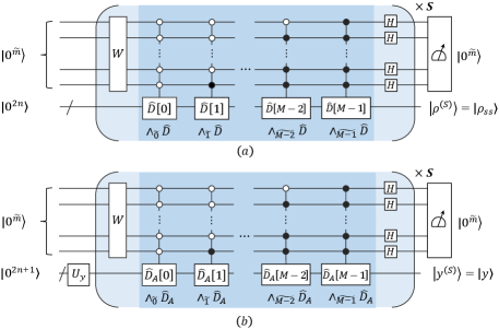
can be estimated from the expectation value of . The Algorithm 1 below and the Fig. (1.a) outline the preparation of NESS with QGD.
Our QGD algorithm requires two quantum registers, the register 1 and register 2. The input is a tensor product state , . The state is an initial guess state picked from easily prepared states such as .
In step 1, we employ the amplitude encoding method to prepare a -qubit input state , where . The preparation takes steps if and can be efficiently computed by classical algorithms Grover2002Creating ; Soklakov2006Efficient . The preparation process can be carried out by applying the following unitary gate on state ,
| (13) |
where the elements are arbitrary so long as is unitary.
In step 2, we implement the -qubit-controlled unitary,
| (14) |
on state to generate the entangled state
| (15) |
The non-unitary gradient operator is realized by an extended unitary gate on a larger Hilbert space.
Without loss of generality, can be expressed as , , where the Pauli operator acts on th qubit. The multi-qubit-controlled unitary gate can be written as
Namely, can be decomposed into multi-qubit-controlled Pauli operators , . Specifically, can be implemented by multiple-qubit-controlled unitary operators.
Last step, we apply Hadamard gates on register 1 and the system state now becomes a separable one,
Suppose that the steps 1-3 are repeated times. The final state of the system is given by
| (16) |
When the register 1 is in state , the state could be a better approximation of the NESS if the satisfies . Otherwise, repeat the overall procedures again until the convergence condition is satisfied. The success probability of obtaining is given by
| (17) |
which decreases exponentially with respect to the number of iterations. Performing quantum amplitude amplification brassard2000quantum , we have that the number of measurements is at most
| (18) |
where and . The final success probability is at least .
III.3 Estimation of expectation values
In addition to focusing on the NESS of open quantum systems, it is also important to provide an efficient scheme to compute expectation values of physical observables. Our algorithm yields a quantum state related to the density matrix . Note that in our approach the state is normalized, i.e., . In general, the condition on the trace is not automatically fulfilled. Thus, the expectation value of an arbitrary observable must be estimated as,
| (19) |
with respect to the density matrix for a given observable . Here, the super-operator and the maximally entangled state
| (20) |
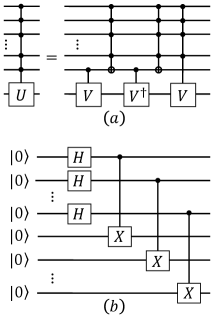
which is prepared by applying the unitary on an initial state . The quantum circuit of the unitary consists of the Hadamard gate and CNOT gate, see Fig. (2.b.) In particular, by setting , the trace of NESS can be calculated by .
We propose two strategies to estimate the expectation value (19) from the output state of the algorithm. While the swap test calculates the square of the inner product buhrman2001quantum ; fanizza2020beyond , the magnitude and sign of the inner product are also required in our specific cases.
Strategy 1. Our first strategy calculates the real and imaginary parts separately based on the modified swap test zhao2019quantum or Hadamard test aharonov2008a .
Start with an initial state with or . We prepare the state by applying the control unitary (see Proposition 1) on the state . After applying the Hadamard gate on the first qubit, we obtain the state
| (21) |
Now we measure the qubit system in the basis of Pauli operator . The measurement output is a random variable , where the output corresponds to the measurement output state . The expectation value of is given by
| (22) |
If , we have . If , then . Let be the probability of measurement outcome . To estimate the probability , we perform independent trials of the Bernoulli test. Then sample times and record the number of observed . The frequency then gives an estimator for up to a sampling error . From Hoeffding’s inequality hoeffding1963 , we have
| (23) |
We obtain the number of measurements, . Therefor we have the following conclusion.
Proposition 1. Let be the controlled unitary gate with and . There exists a quantum algorithm that calculates and to accuracy with success probability at least by using queries of .
Next we estimate the trace average .
Proposition 2. Denote the hermitian operator and the controlled unitary gate with and . The success probability to calculate to accuracy via measuring the expectation value of on state is at least by using queries of .
Proposition 2 can be proved by noting that
| (24) |
due to the structure of the operator . Therefore, similar to the proof of Proposition 1, the number of measurements is .
In the last two Propositions we have assumed that the state can be prepared by applying a unitary on an initial state . However, as shown in Algorithm 1, our state is prepared via a unitary evolution (denoted as ) coupling to a measurement operator . The overall process corresponds to a non-unitary process,
| (25) |
Thus, in order to employ the unitary introduced in the two Propositions, we need to find a unitary to approximate this non-unitary process . Here, we propose a variational quantum non-unitary process approximation to find the unitary . Let be an initial system state. The evolved (normalized) state under the non-unitary operator is given by . The main idea is to train a parameterized quantum circuit , via minimizing an objective function which quantifies the difference between the states and . consists of single-qubit rotation gates and two-qubit CNOT gates havlivcek2019supervised ; commeau2020variational .
Let us have a detailed analysis on the non-unitary approximation algorithm. Our variational quantum non-unitary process approximation outputs a unitary to approximately construct the non-unitary process on a given initial state. A natural objective function is the square of the trace distance between and , i.e.,
which can be evaluated by measuring the expectation of the observable with respect to the state . It is straightforward to verify that the objective function can be expressed as
| (26) |
The objective function is faithful if and only if .
The parameters are trained through a gradient-based optimization method. The optimal parameters can be obtained by updating , where is the learning rate and . The gradient information can be computed on a quantum computer via the finite difference formulae,
| (27) |
where is a small perturbation to . The minimization gives rise to the optimal unitary .
Strategy 2. Our second strategy provides an directly estimation of (19) from the output . Moreover, strategy 2 circumvents local measurement and unitary approximations, thus further reduces the computational complexity.
Proposition 3. Define the hermitian operator and the controlled unitary , with and . Then we can calculate to accuracy via measuring the expectation value of on the state
The success probability is at least by using queries of .
Concerning the proof of Proposition 3 it is straightforward to check that the expectation of the observable is given by
| (28) |
In particular, by setting , the measurement returns to the quantity .
The above strategies do not require the prior knowledge of the spectrum of obtained by quantum phase estimate liang2019quantum and quantum state tomography cramer2010efficient . Thus our approach is experimentally friendly in near-term quantum devices.
III.4 Computational complexity and error analysis
In this section we present the resource complexity and error analysis. The computation complexity contains (1) the gate complexity, the number of the basic quantum gates (single and two qubit gates); (2) the qubit complexity, the number of qubits.
Proposition 4. Concerning the computational complexity of the preparation of , the gate complexity of finding the NESS is , where is the number of decomposition terms of the non-unitary gradient operator and . The qubit complexity is counted as with .
[Proof]. The dominated source of the computational complexity is the controlled unitary in Algorithm 1. The unitary can be simulated by a sequence of single qubit controlled gate and Toffoli gates barenco1995elementary ; Long2006Mathematical ; Wen2020One ; xin2017quantum ; wei2018efficient . Specifically, performing Algorithm 1 one time requires controlled unitary operator . Thus the circuit depth of obtaining NESS is . Under the Pauli decomposition of , the controlled unitary operations can always be rewritten as multi-qubit-controlled Pauli operators , . A general for any unitary matrix can be approximately simulated by a network (Fig. 2.a) including of unitaries , and the Toffoli gate barenco1995elementary . The number of basic operators scales to . Furthermore, the Toffoli gate on qubits can be decomposed into single-qubit and CNOT gates. The unitary operators and can be simulated with a cost . Denote the gate complexity of decomposing . We have the following recurrence relation, , which implies that . Hence, the total gate complexity of simulating is roughly
As shown in Fig. (1.a), the register 2 contains qubits used to store the NESS and the state . The ancillary system requires qubits determined by . Thus the total qubit complexity scales to .
Proposition 5. Concerning the computational complexity of estimating the expectation value , the gate and the qubit complexity are and ( and ) for strategy 1 (strategy 2), respectively.
[Proof]. For both strategies, it is direct to check that the qubit complexity scales to and . The gate complexity for strategy 1 is determined by the parameterized quantum circuit which requires basic quantum gates HardwareVQE2017 ; liang2020variational . Therefore, by using the result of Proposition 4, the total gate complexity for strategy 1 is . For strategy 2, we only require to perform the Algorithm 1 to prepare the state . According to Propositions 3 and 4, we obtain the gate complexity .
Now we determine the upper bound of the error after time iterations. Suppose that the Algorithm 1 runs accurate enough such that
| (29) |
Let be the normalized ideal NESS and the actual state.
Proposition 6. Denote the overlap between an initial state and the state is the largest eigenstate of operator . The approximation error has an upper bound
scaling with , iterations , the gap between largest and lowest eigenvalues of , . and are the two largest eigenstates of the operator .
[Proof]. Consider the eigenvalue decomposition of the hermitian matrix with the eigenvalues arranged in order, . The eigenvalues of are then , . We express the initial state in the basis of the eigenvectors ,
| (30) |
with some coefficients. After applying the non-unitary operator to times, we have
| (31) |
As for all , for larger we can approximate the ground state of as
| (32) |
where the normalization constant
| (33) |
The error satisfies
| (34) |
Therefore, the approximation error has an upper bound scaling with , and .
The above error bound shows that the convergence is geometric with ratio . This implies that the Algorithm 1 would converge slowly if an eigenvalue is close to the dominant eigenvalue of the operator . Hence, one should choose an the initial state with a larger overlap .
The estimation error of the expectation value after time iterations is bounded by a function ,
| (35) |
where denotes the approximation result of . Clearly goes to zero if .
IV QGD for linear algebra problems
In this section, we focus on implementing the QGD algorithm to tackle the linear algebra problems such as solving linear equations and preparing the matrix-vector multiplication states. The core of our strategy is to transform these problems to the simulation of a well-defined Hamiltonian system.
IV.1 QGD for linear equations
Given a sparse matrix and a state vector . The problem is to solve the linear equation . Here, if is not hermitian, one can always transform the problem into an equivalent one with hermitian matrix . The solution can be expressed as . We define the Hamiltonian Subasi2019Quantum ,
| (36) |
where the state . It is easy to check that is the ground state of the Hamiltonian with ground energy , . It is worthwhile to notice that the Hamiltonian has another different form, , as suggested in Xu2020Variational ; LiuWu2021Variational . It can be verified that the solution is the unique eigenstate associated with the minimum eigenvalue zero of .
Concerning the quantum setting in solving the linear equations, let be an efficient Pauli decomposition of the matrix , where , , and are Pauli strings. For classically access to the right-hand side vector we also assume that is an efficient Pauli decomposition of the hermitian matrix , with , and the Pauli strings. The Hamiltonian can then be efficiently encoded,
| (37) |
In order to search the ground state of Hamiltonian , we define the objective function as
| (38) |
It is clear that the minimum of is the desired result with respect to . The gradient of the objective function is given by
| (39) |
Thus the gradient descent iteration can be regraded as the evolution of under the operator ,
| (40) |
where is the learning rate, . Hence, the gradient descent iteration can be also viewed as an evolution of under the non-unitary operator . consists of a polynomial number (with respect to the number of qubits) of tensor products of local Pauli strings, . cannot be implemented directly in quantum circuits as it is not unitary. Such non-unitary evolution can be realized in unitary quantum circuits by adding additional qubits Long2006General ; Cao2010Restricted . We use the following four steps to achieve the iterative process, see Fig. (1.b).
Step 1. Prepare the initial state. The register contains a work system and an ancillary system. At first, one picks an initial vector . The -qubit quantum input state can be prepared by, for instance, employing the amplitude encoding. This encoding uses -qubit to represent vector and requires resources that are polynomial in the number of qubits, if the norm of can be efficiently computed Grover2002Creating ; Soklakov2006Efficient . Note that the exact decomposition of universal gate preparing a general state requires the CNOT gate complexity Bergholm2005Quantum ; Plesch2011Quantum . Another state preparation approach is the quantum random access memory which consumes queries to the oracle that access the element of Giovannetti2008Architectures .
In our iteration algorithm, we only need an easily prepared quantum state, i.e., tensor product state . Then we add qubits and prepare the state by applying the unitary given in (13), where is the normalization constant. The state of the whole system now is
| (41) |
Step 2. Implement the non-unitary operator. We apply a series of ancillary controlled operators,
| (42) |
on the whole state space, where . The whole system state is transformed into
| (43) |
The work qubits and the ancilla qubits are now entangled.
Step 3. Combine the states from different subspaces. We perform Hadamard gates on the ancillary register to combine the states . The system state becomes
| (44) |
Step 4. Measurement. After repeating the above three steps times, the final state of the system is of the form,
| (45) |
Then we measure the former qubits and obtain the classical bits string . The system state collapses to which is an approximate solution of if . Otherwise, we repeat the overall procedures again until the convergence condition is satisfied. The success probability of obtaining the state is given by
| (46) |
which decreases exponentially with respect to the number of iteration steps. Using amplitude amplification brassard2000quantum , we have that measurements are sufficient. Clearly, the qubit complexity is .
IV.2 QGD for matrix-vector multiplication
Given an hermitian matrix and an state , our goal is to prepare the normalized state,
| (47) |
Defining the Hamiltonian Xu2020Variational , one can easily check that the ground state of with ground energy is the state . The expectation value of with respect to an arbitrary state satisfies
| (48) | ||||
| (49) |
where the equality holds if and only if state is the ground eigenstate of . Hence, we define the objection function,
| (50) |
The gradient descent iteration can be regraded as an evolution of under the operator ,
| (51) |
where the non-unitary operator . We only need to substitute the Hamiltonian with and apply the algorithm discussed in last subsection to find the matrix-vector multiplication state . But, here, we require qubits to store and prepare rather than qubits.
In order to estimate the normalization constant
| (52) |
we assume availability of an efficient -qubit quantum circuit such that Huang2019near . The constant (52) is written as
| (53) |
where each term can be evaluated via the Hadamard test aharonov2008a or the measurement on the Pauli basis.
V Numerical experiments
In this section we present some examples to illustrate our approaches.
V.1 The dissipative quantum transverse Ising model
The Hamiltonian of the dissipative quantum transverse Ising model is given by
| (54) |
where are the Pauli operator acting on the -th qubit. The first term denotes the nearest-neighbor spin-spin interaction depending only on the components with coupling strength . The second term accounts for a local and uniform magnetic field along the transverse direction . The site-dependent jump operator (the Lindbald operator) is , and , where . Substitute Eq. (54) into Eq. (III.1), we have for ,
where .
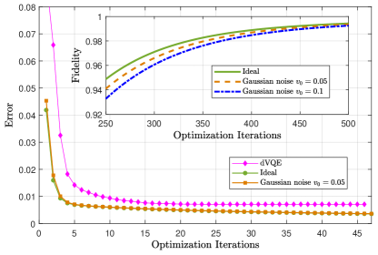
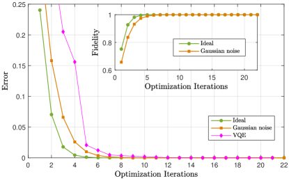
We set , , and the initial state with the learning rate , where . Because of the unavoidable errors in the operations, the non-unitary operator should be substituted by the noise dynamical map . Consider the noise model modeled by a Gaussian noise with variance and mean , . The result error is given by . In Fig. 3 we compare the numerical results of that with and without Gaussian noise. When the optimization iterations increase, the error converges to the minimal value zero in both situations. It is clear that the noise error converges to zero slower than the ideal error. In particular, and for ideal and Gaussian noise (), respectively, with iteration . Another quantity to evaluate our algorithm is the fidelity . The inset of in Fig. (3.a) illustrates that the ideal fidelity is which is higher than the Gaussian noise fidelities () and (), at iteration . Thus, the numerically behavior ensures that our algorithms are robust to Gaussian noise.
Furthermore, we compare our results with the dissipative-system variational quantum eigensolver (dVQE) yoshioka2020variational . In dVQE, the optimization of the loss function starts with a same state . The parameterized quantum circuit
where
| (55) |
and
| (56) |
The rotation operator , , and denotes the complex conjugate of . We apply the classical gradient descent algorithm to optimize the variational parameters. As shown in Fig. (3.a), our results converge faster than dVQE. The minimal error of dVQE is compared with our results (ideal result) or (Gaussian noise, ) at step .
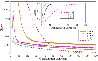
Finally, we perform numerical simulation under different learning rates. As shown in Fig. (3.b), the result error does not converge to the minimal value when . So we should choose the proper learning rate in practical situation.
V.2 Example for matrix-vector multiplication
We now consider the linear equation with
| (57) |
and . Let us consider the case of and the initial state with learning rate , where . The defined Hamiltonian is then encoded in a -qubit system. As , can be expressed as . As a result, the non-unitary operator also has similarly an Pauli decomposition.
With the growth of the number of iterations, Fig. (4) shows that the error of our approach can converges to the local minimum of the objective function. In particular, the fidelity and the error when . Even at the presence of Gaussian noise (), our result still approaches the ideal value, and when . For a comparison we calculate the ground state of by using VQE peruzzo2014variational . As shown in Fig. (4), our result converges faster than that obtained from the VQE.
VI Conclusion and Discussion
In conclusion, based on the quantum gradient descent algorithm we have presented a quantum approach for the (nondegenerate) nonequilibrium steady state problem of open quantum systems. Our method is scalable since the gate and the qubit complexity is polynomial functions of the size of open quantum systems. Capturing the characteristic property of NESS, we introduced two strategies to evaluate the expectation value of the interested physical observable associated with the output state given by vector forms of the density matrix . Furthermore, we have adapted the quantum gradient descent algorithm to solve linear algebra problems including linear equation and matrix-vector multiplications. The basic idea is to convert the linear algebra problems into the simulation of a closed quantum system with a well-defined Hamiltonian. Our quantum linear solver may also serve as a subroutine in solving the Poisson equations with Dirichlet boundary conditions LiuWu2021Variational . On the one hand, the whole optimization procedures of our methods are implemented on a quantum computer. On the other hand, our approach does not need to perform measurements for the expectation values of the Hamiltonian, neither the classical optimization feedbacks, compared with the recent works yoshioka2020variational ; Liu2021Variational . Thus the computational complexity is substantially reduced. Furthermore, different from that the VQAs optimize the cost function in the parameter space, our algorithms optimize the cost function on the original state space. With the increase of the iteration, our algorithm can always obtain a better approximation of the NESS or ground state. Thus another advantage of our strategies is that the barren plateaus do not appear in the quantum gradient descent procedure.
This work focused on the first-order optimization method, but the second-order optimization method (the Newton method) Li2021Quantum may also be used in the preparation of NESS. Aside from the preparation of NESS, it is possible to simulate the dynamics of quantum open systems on a double-dimension Hilbert space. Our approaches highlight the fact that a non-unitary operator composing of local unitary terms may be implemented on NISQ devices. Motivated by the idea of quantum imaginary time evolution Mcardle2019Variational ; Motta2020Determining , approximate simulation of non-unitary evolutions may be possible with a parameterized quantum circuit. Once the optimal parameters are learned, the non-unitary evolution can be carried out by a low-depth quantum circuit which is amenable for NISQ devices. One of the advantages of this strategy is that no any other ancillary systems are required compared with the existing schemes.
Acknowledgements: We would like to thank Dong Liu and Qiao-Qiao Lv for their helpful suggestions and discussions. This work is supported by NSF of China (Grant No. 12075159, 12171044), Beijing Natural Science Foundation (Z190005), Academy for Multidisciplinary Studies, Capital Normal University, the Academician Innovation Platform of Hainan Province, and Shenzhen Institute for Quantum Science and Engineering, Southern University of Science and Technology (No. SIQSE202001). The National Natural Science Foundation of China under Grants No. 12005015.
References
- (1) R. P. Feynman, Int. J. Theor. Phys. 21, 467 (1982).
- (2) A. M. Childs, and N. Wiebe, Quantum Info. Comput. 12, 901 (2012).
- (3) D. Bacon and W. van Dam, Commun. ACM 53, 84 (2010).
- (4) T. Xin, L. Hao, S.-Y. Hou, G.-R. Feng and G.-L. Long, Sci. China Phys. Mech. Astron. 62, 960312(2019).
- (5) C. Yang, D. X. Li and X. Q. Shao, Sci. China Phys. Mech. Astron. 62, 110312 (2019).
- (6) H.-S. Li, P. Fan, H. Xia, H. Peng and G.-L. Long, Sci. China Phys. Mech. Astron. 63, 280311 (2020).
- (7) Z.-D. Ye, D. Pan, Z. Sun, C.-G. Du, L.-G. Yin and G.-L. Long, Front. Phys. 16, 21503 (2021).
- (8) S.-J. Ran, Z.-Z Sun, S.-M. Fei, G. Su and M. Lewenstein, Phys. Rev. Research 2, 033293 (2020).
- (9) P. Shor, in Proceedings of 35th Annual IEEE Symposium on Foundations of Computer Science (IEEE, Piscataway, 1994), pp. 124-134.
- (10) L. K. Grover, Phys. Rev. Lett. 79, 325 (1997).
- (11) A. W. Harrow, A. Hassidim, and S. Lloyd, Phys. Rev. Lett. 103, 150502 (2009).
- (12) J. Biamonte, P. Wittek, N. Pancotti, P. Rebentrost, N. Wiebe, and S. Lloyd, Nature 549, 195 (2017).
- (13) P. Krantz, M. Kjaergaard, F. Yan, T. P. Orlando, S. Gustavsson, and W. D. Oliver, Appl. Phys. Rev. 6, 021318 (2019).
- (14) H.-L. Huang, D. Wu, D. Fan, and X. Zhu, Sci. China Inf. Sci. 63, 180501 (2020).
- (15) Y. Wu, W.-S. Bao, S. Cao et al., Phys. Rev. Lett. 127, 180501 (2021).
- (16) S. Slussarenkoa and G. J. Pryde, Appl. Phys. Rev. 6, 041303 (2019).
- (17) C. H. Yang, K. W. Chan, R. Harper, W. Huang, T. Evans, J. C. C. Hwang, B. Hensen, A. Laucht, T. Tanttu, F. E. Hudson, S. T. Flammia, K. M. Itoh, A. Morello, S. D. Bartlett, and A. S. Dzurak, Nat Electron 2, 151 (2019).
- (18) R. Blatt and C. F. Roos, Nature Phys 8, 277 (2012).
- (19) C. D. Bruzewicza, J. Chiaverinib, R. McConnellc, and J. M. Saged, Appl. Phys. Rev. 6, 021314 (2019).
- (20) J. Preskill, Quantum 2, 79 (2018).
- (21) R. LaRose, A. Tikku, É. O’Neel-Judy, L. Cincio, and P. J.Coles, npj Quantum Inform. 5, 8 (2019).
- (22) A. Peruzzo, J. McClean, P. Shadbolt, M.-H. Yung, X.-Q. Zhou, P. J. Love, A. Aspuru-Guzik, and J. L. O’Brien, Nat. Commun. 5, 4213 (2014).
- (23) O. Higgott, D. Wang, and S. Brierley, Quantum 3, 156 (2019).
- (24) T. Jones, S. Endo, S. McArdle, X. Yuan, and S. C. Benjamin, Phys. Rev. A 99, 062304 (2019).
- (25) X. Wang, Z. Song, Y. Wang, Quantum 5, 483 (2021).
- (26) M. Benedetti, E. Lloyd, S. Sack, and M. Fiorentini, Quantum Sci. Technol. 4, 043001 (2019).
- (27) K. Li, S. Wei, P. Gao, F. Zhang, Z. Zhou, T. Xin, X. Wang, P. Rebentrost, and G. Long, npj Quantum Inf 7, 16 (2021).
- (28) J. Liu, K. H. Lim, K. L. Wood, W. Huang, C. Guo, and H.-L. Huang, Sci. China Phys. Mech. Astron. 64, 290311 (2021).
- (29) J.-M. Liang, S.-Q. Shen, M. Li, and S.-M. Fei, Quantum Inf. Process. 21, 23 (2022).
- (30) H.-L. Huang, Y. Du, M. Gong et al. Phys. Rev. Applied 16, 024051 (2021).
- (31) Vojtěch Havlíček, A. D. Córcoles, K. Temme, A. W. Harrow, A. Kandala, J. M. Chow, and J. M. Gambetta, Nature 567, 209 (2019).
- (32) M. P. Harrigan, K. J. Sung, M. Neeley et al. Nat. Phys. 17, 332 (2021).
- (33) S. Wei, H. Li, and G. Long, Research 2020, 1 (2020).
- (34) G. L. Long, Commun. Theor. Phys. 45, 825 (2006).
- (35) H. Fan, Sci. China Phys. Mech. Astron. 64, 100332 (2021).
- (36) S. Diehl, A. Micheli, A. Kantian, B. Kraus, H. P. Büchler, and P. Zoller, Nat. Phys. 4, 878 (2008).
- (37) F. Verstraete, M. M.Wolf, and J. I. Cirac, Nat. Phys. 5, 633 (2009).
- (38) I. Rotter, J. Phys. A: Math. Theor. 42, 153001 (2009).
- (39) H. P. Breuer and F. Petruccione, The Theory of Open Quantum Systems (Oxford University Press, Oxford, 2002).
- (40) J. Han, W. Cai, L. Hu, X. Mu, Y. Ma, Y. Xu, W. Wang, H. Wang, Y. P. Song, C.-L. Zou, and L. Sun, Phys. Rev. Lett. 127, 020504 (2021).
- (41) S.-J. Wei, D. Ruan, and G.-L. Long, Sci. Rep 6, 30727 (2016).
- (42) B. Kraus, H. P. Buchler, S. Diehl, A. Kantian, A. Micheli, and P. Zoller, Phys. Rev. A 78, 042307 (2008).
- (43) S. Diehl, E. Rico, M. A. Baranov, and P. Zoller, Nat. Phys. 7, 971 (2011).
- (44) A. Nagy and V. Savona, Phys. Rev. Lett. 122, 250501 (2019).
- (45) M. J. Hartmann and G. Carleo, Phys. Rev. Lett. 122, 250502 (2019).
- (46) F. Vicentini, A. Biella, N. Regnault, and C. Ciuti, Phys. Rev. Lett. 122, 250503 (2019).
- (47) N. Yoshioka, Y. O. Nakagawa, K. Mitarai, and K. Fujii, Phys. Rev. Research 2, 043289 (2020).
- (48) H.-Y. Liu, T.-P. Sun, Y.-C. Wu and G.-P. Guo, Chin. Phys. Lett. 38 080301 (2021).
- (49) P. Rebentrost, M. Schuld, L. Wossnig, F. Petruccione, and S. Lloyd, New J. Phys. 21, 073023 (2019).
- (50) A. Kandala, A. Mezzacapo, K. Temme, M. Takita, M. Brink, J. M. Chow, and J. M. Gambetta, Nature 549, 242 (2017).
- (51) R. M. Parrish, E. G. Hohenstein, P. L. McMahon, and T. J. Martánez, Phys. Rev. Lett. 122, 230401 (2019).
- (52) S. Lloyd and C. Weedbrook, Phys. Rev. Lett. 121, 040502 (2018).
- (53) P.-L. Dallaire-Demers and N. Killoran, Phys. Rev. A 98, 012324 (2018).
- (54) P. Gao, K. Li, S. Wei, J. Gao, and G. Long, Phys. Rev. A 103, 042403 (2021).
- (55) G. Lindblad, Commun. Math. Phys. 48, 119 (1976).
- (56) M. Mahdian and H. D. Yeganeh, J. Phys. A: Math. Theor. 53 415301 (2020).
- (57) S. Lloyd, Science 273, 1073 (1996).
- (58) N. Yoshioka and R. Hamazaki, Phys. Rev. B 99, 214306 (2019).
- (59) H. Kamakari, S.-N. Sun, M. Motta, and A. J. Minnich, arXiv:2104.07823.
- (60) T. F. Havel, J. Math. Phys 44, 534 (2003).
- (61) F. Minganti, A. Biella, N. Bartolo, and C. Ciuti, Phys. Rev. A 98, 042118 (2018).
- (62) S. G. Schirmer and X.Wang, Phys. Rev. A 81, 062306 (2010).
- (63) L. Grover and T. Rudolph, arXiv:quant-ph/0208112.
- (64) A. N. Soklakov and R. Schack, Phys. Rev. A 73, 012307 (2006).
- (65) G. Brassard, P. Hoyer, M. Mosca, A. Tapp, Contemp. Math. 305, 53 (2002).
- (66) H. Buhrman, R. Cleve, J. Watrous, and R. de Wolf,Phys. Rev. Lett. 87, 167902 (2001).
- (67) M. Fanizza, M. Rosati, M. Skotiniotis, J. Calsamiglia, and V. Giovannetti, Phys. Rev. Lett. 124, 060503 (2020).
- (68) Z. Zhao, J. K. Fitzsimons, and J. F. Fitzsimons, Phys. Rev. A 99, 052331 (2019).
- (69) D. Aharonov, V. Jones, and Z. Landau, Algorithmica 55, 395 (2009).
- (70) W. Hoeffding, J. Am. Stat. Assoc. 58, 13 (1963).
- (71) B. Commeau, M. Cerezo, Z. Holmes, L. Cincio, P. J. Coles, A. Sornborger, arXiv:2009.02559.
- (72) J.-M. Liang, S.-Q. Shen, M. Li, and L. Li, Phys. Rev. A 99, 052310 (2019).
- (73) M. Cramer, M. B. Plenio, S. T. Flammia, R. Somma, D. Gross, S. D. Bartlett, O. Landon-Cardinal, D. Poulin, and Y.-K. Liu, Nat. Commun. 1, 149 (2010).
- (74) G. L. Long, Quantum Inf. Process. 6, 49 (2007).
- (75) J. W. Wen, X.C. Qiu, X.Y. Kong, X.Y. Chen, F. Yang, and G.L. Long, Sci. China Phys. Mech. Astron. 63, 230321 (2020).
- (76) A. Barenco, C. H. Bennett, R. Cleve, D. P. DiVincenzo, N. Margolus, P. Shor, T. Sleator, J. A. Smolin, and H. Weinfurter, Phys. Rev. A 52, 3457 (1995).
- (77) T. Xin, S.-J. Wei, J. S. Pedernales, E. Solano, and G.-L. Long, Phys. Rev. A 96, 062303 (2017).
- (78) S.-J. Wei, T. Xin, and G.-L. Long, Sci. China Physics, Mech. Astron., 61, 70311 (2018).
- (79) J.-M. Liang, S.-Q. Shen, M. Li, and L. Li, Phys. Rev. A 101, 032323 (2020).
- (80) Y. Subasi and R. D. Somma, Phys. Rev. Lett. 122, 060504 (2019).
- (81) X. Xu, J. Sun, S. Endo, Y. Li, S. C. Benjamin, X. Yuan, arXiv:1909.03898.
- (82) H.-L. Liu, Y.-S. Wu, L.-C. Wan, S.-J. Pan, S.-J. Qin, F. Gao, and Q.-Y. Wen, Phys. Rev. A 104, 022418 (2021).
- (83) H. X. Cao, L. Li, Z. L. Chen, Y. Zhang, and Z. H. Guo, Chinese Science Bulletin, 55, 2122 (2010).
- (84) V. Bergholm, J. J. Vartiainen, M. Möttönen, and M. M. Salomaa, Phys. Rev. A 71, 052330 (2005).
- (85) M. Plesch and Č. Brukner, Phys. Rev. A 83, 032302 (2011).
- (86) V. Giovannetti, S. Lloyd, and L. Maccone, Phys. Rev. A 78, 052310 (2008).
- (87) H.-Y. Huang, K. Bharti, and P. Rebentrost, arXiv:1909.07344.
- (88) P. Gao, K. Li, S. Wei, and G.-L. Long, Sci. China Phys. Mech. Astron. 64, 100311 (2021).
- (89) S. McArdle, T. Jones, S. Endo, Y. Li, S. C. Benjamin, and X. Yuan, npj Quantum Inf 5, 75 (2019).
- (90) M. Motta, C. Sun, A. T. K. Tan, M. J. O’Rourke, E. Ye, A. J. Minnich, F. G. S. L. Brandão, and G. K.-L. Chan, Nat. Phys 16, 205 (2020).