Quantum measurement process with an ideal detector array
Abstract
Any observable with finite eigenvalue spectrum can be measured using
a multiport apparatus realizing an appropriate unitary transformation
and an array of detector instruments, where each detector operates
as an indicator of one possible value of the observable. The study
of this setup in the frame of von Neumann’s quantum mechanical measurement
process has a remarkable result: already after the interaction of
the measured system with the detector array without collapse, exactly
one detector is indicating a detection. Each single detector indicates
either 0 or 1 detection, and no superposition can be attributed to
it.
Keywords: Measurement process Detector array
Definite outcome Preferred base Wave function collapse
1 Introduction
Reck et al. (1994) demonstrated that any finite dimensional unitary transformation can be realized in the laboratory using a lossless multiport apparatus constructed with beam splitters, mirrors, and phase shifters. Furthermore, any finite dimensional observable can be measured realizing an appropriate unitary transformation, attaching a particle source to the input port and particle detectors to the output ports. In this case, each detector operates as an indicator of one possible value of the observable.
Measurement instruments of this type are used in many modern versions of quantum mechanical experiments. The authors list Einstein-Podolsky-Rosen (Einstein et al., 1935; Bohm and Aharonov, 1957) and Bell test (Bell, 1964; Clauser et al., 1969) experiments, as well as variants of Stern-Gerlach experiments (Gerlach and Stern, 1922), and quantum cryptography devices (Ekert, 1991). A famous example is Aspect’s Bell test experiment (Aspect et al., 1982) with photons, which was repeated in many variants, even with neutrons (Hasegawa et al., 2003). Several other experiments with neutrons (in line with their photon counterparts) are described in (Sponar et al., 2021), with many additional references.
In the following, such measurement instruments are considered theoretically, with a focus on the detectors, which are treated quantum mechanically in the frame of von Neumann’s measurement process (v. Neumann, 1932; Wheeler and Zurek, 1983). Any observable with finite eigenvalue spectrum can be measured with an array of detector instruments using an appropriate measurement interaction, described by a unitary transformation, which fulfills the conditions for a repeatable ideal measurement. It is well-known, that this interaction of the measured system and the measurement instrument ends with an entangled state, which exhibits the “measurement problem”: how to get a definite outcome. Schrödinger’s cat, waiting in a killing machine triggered by the measurement outcome, is iconic for this situation: is it dead, alive, or in a superposition of these states? For the Copenhagen interpretation (Heisenberg, 1958), the measurement must be completed by some final reduction or collapse (Busch et al., 1991) to get a definite outcome. However, with the detector array the entangled state already has some special properties, which are usually assumed to arise with the collapse: exactly one detector is indicating a detection; each single detector indicates either 0 or 1 detection, and no superposition can be attributed to it.
2 Von Neumann’s measurement process
Von Neumann (1932) described the measurement process quantum mechanically as a short time interaction between the measured system and a measurement instrument , using Hilbert space and , respectively, as state space, and the tensor product for the composite system . The instrument has to display the measurement outcome by entering one of the pairwise orthogonal pointer states , which correspond to the eigenvalues of the measured observable (assumed to be bounded and to have a pure, non-degenerate eigenvalue spectrum). The initial state of the composite system before the interaction and its final state after that are connected by a unitary transformation , which must fulfill two conditions to constitute a repeatable ideal measurement of the observable : any eigenstate of stays unchanged, and the instrument must enter the corresponding pointer state , indicating the measurement of the eigenvalue , i.e.
| (1) |
with as the initial state of the instrument. As a consequence, the interaction of the measurement instrument in initial state with a system in state
with , transforms the composite system into the entangled state
with probability to observe the pointer , according to Born’s rule. This superposition of products of eigenstates and corresponding pointer states exhibits the “measurement problem”, how to get a definite outcome, and is a reason for different interpretations of quantum mechanics (Mittelstaedt, 1998). According to the Copenhagen interpretation, however, this state terminates only the “premeasurement” (Busch et al., 1991). The measurement must be completed by some additional reduction or collapse, giving a definite outcome in a random, irreversible transition
where is the pointer state indicating the definite outcome , the corresponding eigenstate of the measured system and the transition probability. Different authors associate this transition with different circumstances, e.g. the recognition of the measurement outcome by a conscious observer (Wigner, 1961) or its registration by a classical device (Bohr, 1958). Some non-Copenhagen interpretations (e.g. the pilot wave interpretation (Bohm, 1952a, b), the many-worlds interpretation (Everett, 1957)) deny such an additional transition at all and assume that the final premeasurement state already constitutes the end of the measurement.
The state of the system after reduction is an eigenstate of , so a repetition of the measurement will give the same outcome . However, as Pauli (1933) already noticed, there are ideal measurements for which an immediate repetition gives not the same result. The measurement scheme of the multiport apparatus with detectors (Reck et al., 1994) is of this type. Von Neumann’s conditions (1) must be relaxed to describe such non-repeatable ideal measurements (Busch et al., 1991): an eigenstate will be transformed into another state , while the instrument enters the corresponding pointer state
| (2) |
For the multiport apparatus we can write , with the unitary transformation determined by the apparatus. Here, these are not eigenstates of but of the observable
| (3) |
measured repeatably by the detectors. The collapse of the final premeasurement state gives then
| (4) |
indicating the measurement outcome , with the system in the state .
3 Premeasurement with an ideal detector
In the following, an ideal detector is considered as an instrument for measuring an indicator observable (binary observable) which is represented by a projection operator with , eigenvalues , and the complement . A suitable detector instrument has at least orthogonal pointer states to display the measurement result. With Hilbert space , the detector instrument can be a spin-1/2-system or a qubit.
The mathematical expression of von Neumann’s conditions (1) for the interaction must be generalized to include repeatable ideal measurements of degenerate observables (Lüders, 1951). For an arbitrary vector , and are (unnormalized) eigenvectors of (or the zero vector) with eigenvalues or respectively. So, the conditions are
| (5) |
for all .
Example 1
Premeasurement with a detector.
a) A vector of the Hilbert space can be written as 2-component column vector (similar as a spinor). In this notation, the matrix
with , fulfills the conditions
for a repeatable ideal measurement (5).
b) If the measured system is a spinless particle, with ,
an indicator observable for position detection is the indicator function
, with ,
of a Borel set representing the detection
volume (in position representation), with
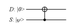
c) If the measured system is a qubit (Nielsen and Chuang, 2000), with a indicator observable for a measurement in the computational base is
and with its matrix representation one gets a matrix for the measurement transformation
which is a representation of a CNOT circuit with 2 qubits (fig. 1).
4 Premeasurement with an ideal detector array
Any observable with a finite eigenvalue spectrum can be written as a linear combination of projection operators onto the eigenspaces
with
| (6) |
for all , and
| (7) |
The projection operators are indicator observables for the corresponding eigenvalues and can be measured using ideal detector instruments , assuming a bijection
| (8) |
An array of these detectors can be used as a measurement instrument for the observable . With pointer states , of detector , the pointer states of this instrument are
for , in Hilbert space . The measurement result is the index of the detector with the pointer state , equivalent to the pointer state of the whole array, indicating the value of the observable . Here, von Neumann’s conditions (1) for an repeatable ideal measurement of observable are
| (9) |
for all and .
In the rest of this paragraph, a construction for this unitary transformation is given, using the detector transformation from (5) for each single detector . With (6) we can write (5)
| (10) |
for all , and can be constructed as product
where
is the representation of in the product space It is obvious, that these operators commute
for all . To demonstrate that fulfills von Neumann’s conditions for the eigenstates of , we multiply the initial state of the composite system
for each successively with using (10)
which gives (9).
Example 2
Premeasurement with a 2-detector array.
a) With the indicator observables the matrix representation of from Example 1 gives
which fulfills (9).
b) If the measured system is a particle, the Hilbert space can
be restricted to a finite box ,
with . Then, the completeness
condition (7) for the partition of the position
space can be fulfilled with two finite detection
volumes and the corresponding indicator functions ,
in position representation. Such partitions give
a simple model of a tracking chamber.
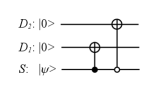
c) If the measured system is a qubit, the measurement interaction
for a measurement in the computational base with
and can be
described with the resulting matrix for
or, equivalently, with an -to- decoder circuit (fig. 2).
5 Properties of the final premeasurement state
It is a consequence of (7) and the conditions (9), that for an arbitrary initial state of the measured system the final premeasurement state of the composite system is
To include non-repeatable ideal measurements with the multiport apparatus (2), we discuss the more general final premeasurement state
| (11) |
where is a projection operator for all , defined by the inverse transformation of (3).
This entangled state of the system and the detector array has several interesting properties.
5.1 Exactly one detection
An observable of the detector array is the number of detectors indicating a detection . With the eigenvalue spectrum it can be written as
with projection operators onto the closed subspaces spanned by the vectors
It is obvious that is an eigenvector of with eigenvalue and are eigenvectors with eigenvalue . Consequently, the final premeasurement state (11) is an eigenstate of with eigenvalue 1
So, the observable has in state the dispersion free expectation value . This means, exactly one detector is indicating a detection.
5.2 Preferred pointer base states
The biorthogonal Schmidt decomposition of an entangled state is in general not unique (Schlosshauer, 2004; Ekert and Knight, 1995). Consequently, the same entangled state can arise as a final premeasurement state measuring incompatible observables. However, with the final premeasurement state (11), only eigenstates of the number operator with eigenvalue can be used as factors for the detector array. This can be shown considering the alternative Schmidt decomposition
Because of the pairwise orthogonality, each summand must be zero. Therefore, each has to be an eigenstate of with eigenvalue .
There is no factorization of such an eigenstate with other single detector states than the pointer states ,. To see this, let be an eigenvector of the number operator with eigenvalue and
a factorization with . Then, we can write
with and , and
Non-trivial equality is only possible with and or with and . Since the factorization of the state
is a factorization of all , it is only possible with or .
For a single detector of the array, with , this has the consequence that no superposition of the pointer states and can be attributed to the final premeasurement state (11) as a factor of a Schmidt decomposition. The pointer base states are preferred (Zurek, 2003) and the reduced state of each detector is a unique mixture of and .
5.3 Conditional expectations equal expectations after collapse
Other studies (Laura and Vanni, 2008) have shown, that for an ideal repeatable measurement, fulfilling von Neumann’s conditions, the final premeasurement state gives the same conditional probabilities for the measured system as the collapse of the wave function. This is also the case with the collapse of the premeasurement state after a non-repeatable ideal measurement (4).
To see this for state (11) let be the indicator observable for detection by detector , i.e. the projection operator onto . It commutes with all system observables. So, a common probability space is available for all these observables and the conditional probability of any event represented by the indicator observable of the system, given , is well defined for all
if . This is a consequence of Born’s rule. The state of the system after the complete measurement with collapse, given the outcome , is according to (4)
For this state the probability of is
and has the same value as the conditional probability of , given , for the state . The same is valid for the conditional expectation value of any observable of the system.
Consequently, considering the Heisenberg picture, the isolated evolution of the system after the measurement interaction, given , is the same as for the collapsed wave function after the measurement, given the outcome .
6 Conclusion
The entangled state of the system and the detector array after the ideal premeasurement of an observable has the remarkable property that the number of detectors indicating a detection is exactly one. This is a hint at a definite outcome of the measurement and resembles the collapse, since the conditional expectations, given a detection, are the same as for the collapsed state, given the corresponding outcome. Furthermore, no superposition state can be attributed to a single detector: the pointer base states and their mixtures are preferred.
Using Schrödinger’s cat illustration, one can say: if in a lossless multiport experiment a particle has different exits for all possible measurement outcomes, each one with an ideal detector connected to a killing machine with its own cat, then exactly one cat will be dead, and all others will be alive after a trial; there is no superposition of dead and alive – even after a pure unitary evolution without collapse.
These properties depend on an ideal measurement process where the detector array fulfills the completeness and orthogonality conditions (7), (6) with the bijection (8). Quantum computing circuits (example 2c) demonstrate the possibility of such a setting. In case of position detectors (example 2b), exactly positioned detection volumes without gap and overlap, filling the available space, are required, which seams only possible in a macroscopic quasi-classical limit, in line with Bohr’s Copenhagen (Bohr, 1958) interpretation.
Solely, these properties cannot constitute irreversible facts. That, however, could be accomplished through the decoherence of the final premeasurement state (Schlosshauer, 2004).
The results of our study may support interpretations of quantum mechanics without collapse. However, if some of the latter’s observable consequences are deducible from other rules, this will not mean a contradiction to the Copenhagen interpretation. Even, if the collapse postulate was rendered unnecessary, it could persist as useful rule of thumb.
References
- Aspect et al. [1982] A. Aspect, J. Dalibard, and G. Roger. Experimental test of Bell’s inequalities using time-varying analyzers. Phys. Rev. Lett., 49, 1982. doi: 10.1103/PhysRevLett.49.91.
- Bell [1964] J. S. Bell. On the Einstein-Podolsky-Rosen paradox. Physics, 1, 1964. doi: 10.1017/CBO9780511815676.004.
- Bohm [1952a] D. Bohm. A suggested interpretation of the quantum theory in terms of ’hidden’ variables. I. Phys. Rev., 85, 1952a. doi: 10.1103/PhysRev.85.166.
- Bohm [1952b] D. Bohm. A suggested interpretation of the quantum theory in terms of ’hidden’ variables. II. Phys. Rev., 85, 1952b. doi: 10.1103/PhysRev.85.180.
- Bohm and Aharonov [1957] D. Bohm and Y. Aharonov. Discussion of Experimental Proof for the Paradox of Einstein, Rosen, and Podolsky. Phys. Rev., 108, 1957. doi: 10.1103/PhysRev.108.1070.
- Bohr [1958] N. Bohr. Quantum Physics and Philosophy - Causality and Complementarity. In R. Klibansky, editor, Philosophy in the Mid-Century. La nuova Italia Editrice, Florence, 1958.
- Busch et al. [1991] P. Busch, P. J. Lahti, and P. Mittelstaedt. The Quantum Theory of Measurement. Springer-Verlag, Berlin, 1991.
- Clauser et al. [1969] J. F. Clauser, M. A. Horne, A. Shimony, and R. A. Holt. Proposed experiment to test local hidden-variable theories. Phys. Rev. Lett., 23, 1969. doi: 10.1103/PhysRevLett.23.880.
- Einstein et al. [1935] A. Einstein, B. Podolsky, and N. Rosen. Can quantum-mechanical description of physical reality be considered complete? Phys. Rev., 47, 1935. doi: 10.1103/PhysRev.47.777.
- Ekert [1991] A. K. Ekert. Quantum cryptography based on Bell’s theorem. Phys. Rev. Lett., 67, 1991. doi: 10.1103/PhysRevLett.67.661.
- Ekert and Knight [1995] A. K. Ekert and P. L. Knight. Entangled quantum systems and the Schmidt decomposition. Am. J. Phys., 63, 1995. doi: 10.1119/1.17904.
- Everett [1957] H. Everett. "relative state" formulation of quantum mechanics. Rev. Mod. Phys., 29, 1957. doi: 10.1103/RevModPhys.29.454.
- Gerlach and Stern [1922] W. Gerlach and O. Stern. Der experimentelle Nachweis der Richtungsquantelung im Magnetfeld. Z. Physik, 9, 1922. doi: 10.1007/BF01326983.
- Hasegawa et al. [2003] Y. Hasegawa, R. Loidl, G. Badurek, M. Baron, and H. Rauch. Violation of a bell-like inequality in single-neutron interferometry. Nature, 425, 2003. doi: 10.1038/nature01881.
- Heisenberg [1958] W. Heisenberg. Physics and Philosophy. Penguin Classics, Reprint, 1958.
- Laura and Vanni [2008] R. Laura and L. Vanni. Conditional probabilities and collapse in quantum measurements. Int. Journal of Theor. Phys., 47, 2008. doi: 10.1007/s10773-008-9672-7.
- Lüders [1951] G. Lüders. Über die Zustandsänderung durch den Messprozess. Ann. d. Physik, 1951. doi: 10.1002/andp.200610207.
- Mittelstaedt [1998] P. Mittelstaedt. The Interpretation of Quantum Mechanics and the Measurement Process. Cambridge University Press, 1998.
- Nielsen and Chuang [2000] M. Nielsen and I. L. Chuang. Quantum Computation and Quantum Information. Cambridge University Press, 2000.
- Pauli [1933] W. Pauli. Die allgemeinen Prinzipien der Wellenmechanik. Springer-Verlag, Berlin, 1933.
- Reck et al. [1994] M. Reck, A. Zeilinger, H. J. Bernstein, and P. Bertani. Experimental realization of any discrete unitary operator. Phys. Rev. Lett., 73, 1994. doi: 10.1103/PhysRevLett.73.58.
- Schlosshauer [2004] M. Schlosshauer. Decoherence, the measurement problem, and interpretation of quantum mechanics. Rev. Mod. Phys., 76, 2004. doi: 10.1103/RevModPhys.76.1267.
- Sponar et al. [2021] S. Sponar, R. I. P. Sedmik, and M. Pitschmann. Tests of fundamental quantum mechanics and dark interactions with low-energy neutrons. Nat. Rev. Phys., 3, 2021. doi: 10.1038/s42254-021-00298-2.
- v. Neumann [1932] J. v. Neumann. Mathematische Grundlagen der Quantenmechanik. Springer-Verlag, Berlin, 1932.
- Wheeler and Zurek [1983] J. A. Wheeler and W. H. Zurek, editors. Quantum Theory and Measurement. Princeton University Press, Princeton, 1983.
- Wigner [1961] E. P. Wigner. Remarks on the mind body question. In I. J. Good, editor, The Scientist Speculates. William Heinemann, Ltd., London, 1961.
- Zurek [2003] W. H. Zurek. Decoherence, einselection, and the quantum origins of the classical. Rev. Mod. Phys., 75, 2003. doi: 10.1103/RevModPhys.75.715.