Quantum phase transition of Bose-Einstein condensates on a ring nonlinear lattice

In the absence of atomic interactions, the ground state is quite trivial: all the atoms occupy the zero-momentum mode $\widehat{a}_{0}$. In the presence of interaction, this is no longer true. However, we may conjecture that the system condenses into a different ground mode $\widehat{\chi}_{0}$. This mode $\widehat{\chi}_{0}$, together with other orthogonal modes $\{\widehat{\chi}_{i}\}$’s that form a complete set, are related to the $\{\widehat{a}_{i}\}$ modes through a unitary transformation $U$:

In terms of $\{\widehat{\chi}_{i}\}$ and $\{\widehat{\chi}_{i}^{\dagger}\}$, the biquadratic Hamiltonian in Eq. (4) takes the following form:

This Hamiltonian can be simplified by a few considerations. First, it is assumed that most atoms will be in the condensate mode $\widehat{\chi}_{0}$. Under the mean field approximation, operators for the macroscopically occupied condensate mode are replaced by $c$-numbers, i.e., $\widehat{\chi}_{0},\widehat{\chi}_{0}^{\dagger}\rightarrow\sqrt{N}$. Since occupation numbers in other $\widehat{\chi}_{k}$ modes are very small, we can drop terms involving 3 or more operators in $\widehat{\chi}_{k}$ and $\widehat{\chi}_{k}^{\dagger}$ for $k\neq 0$. After this exercise, we obtain the following effective Hamiltonian up to second order in $\{\widehat{\chi}_{k}\}$ and $\{\widehat{\chi}_{k}^{\dagger}\}$:

This effective Hamiltonian can be diagonalized by the Bogoliubov transformation and the system’s elementary excitaitons are quasiparticles in nature. In order to investigate the stability of the system, we need to analyze the energy spectrum of these quasiparticle excitations. For this purpose, we should work with the following grand canonical operator to acccount for the conservation of atom numbers:

Here, $\mu$ is the chemical potential and can be calculated from the condensate energy $E=\left\langle H\right\rangle\approx c_{0}N$ as:

Now, we may diagonalize the operator $K$ by using the Bogoliubov transformation on $\{\widehat{\chi}_{k}\}$ and $\{\widehat{\chi}_{k}^{\dagger}\}$ and obtain the excitation spectrum of quasiparticles. (This will be elaborated on later.) If there is no imaginary excitation frequencies, we claim that the condensate mode $\widehat{\chi}_{0}$ is dynamically stable.

In the above prescription, the key step is to search for the appropriate unitary transformation defined in Eq. (5) that transforms Hamiltonian (4) into (6). Although there are a great number of unknown parameters in the undetermined unitary matrix $U$, further analysis shows that only the elements in the first row of $U$ are necessary for determining the form of the Hamiltonian (6).

To see this, we note that in order to transform Hamiltonian (4) into (6) via the unitary matrix $U$, a fundamental requirement is to maintain the biquadratic terms of the operators $\left(\widehat{\chi}_{0}^{\dagger},\widehat{\chi}_{0}\right)$ and to eliminate all the cubic terms. To this end, we may use the operators $\left(\widehat{\chi}_{i}^{\dagger},\widehat{\chi}_{j}\right)$ to represent the operators $\left(\widehat{a}_{l}^{\dagger},\widehat{a}_{m}\right)$ in Hamiltonian (4) via:

where $u_{ij}$ is the matrix element of the unitary matrix $U$, and we obtain the following two equations :

Since $\chi_{0}=\sum_{i}u_{0i}a_{i}$, Eq. (11) can be recast into a set of equations in operators $\left\{a_{i}\right\}$ (the number of this set of equations depends on the cut-off of the Bose modes) and can be solved by numerical method. Once the representation of the operator $\chi_{0}$ is determined, the parameter $c_{0}$ and the chemical potential $\mu$ can be obtained by solving Eqs. (10) and (9), respectively. Therefore, Eqs. (10) and (11) together represent an algebraic form of the Gross-Pitaevskii (GP) equation. In Appendix A, we will show that they are indeed equivalent to the ordinary GP equation. The main advantage of Eqs. (10) and (11) is that, in principle, all the stationary states (both dynamically stable and unstable ones) of the system can be found. When more than one stable solutions are found, the one that is dynamically stable and with the lowest energy will be identified as the ground state of the system. In contrast, with ordinary GP equation, using imaginary time evolution method one can only find the dynamically stable states, and often just the ground state. Therefore, Eqs. (10) and (11) are supeior for studying the phase transitions in our system, where information beyond the ground state is needed.

Once the condensate state is determined, the Bogoliubov spectrum of quasiparticle excitations above it can be found by diagonalizing $K$ defined in Eq. (8) using the Bogoliubov transformation. The details are described in Appendix B.

Using the modified Bogoliubov method outlined in the previous section, in principle we can find all the stationary states (not just the ground state) and their excitation spectrum for any modulated atomic interactions. This provides a more thorough picture of the energy landscape of the system and deeper insights into possbile quantum phase transitions induced when certain parameters are varied (in our case, the modulation depth of the interaction strength $\gamma_{0}$).

Our goal is to study the mean field quantum phase transition for different modulation period $d$ as the modulation depth $\gamma_{0}$ is varied. We concentrate on the low-energy states, meaning stationary states with energy close to that of the ground state. We find that there are mainly two types of stationary states in the low energy regime. One type has a density profile matching the modulated period of the scattering length. We refer to such states as symmetric states. The other type features a density profile that spontaneously breaks the symmetry of the modulation. We refer to such states as asymmetric states. The asymmetric states is always $d$-fold degenerate with the peak density located at $\frac{(1+4i)\pi}{2d}$ ($i=0,1,...d-1$), where the local interaction energy $U(\theta)$ reaches the minimum. Under the mean field treatment (MFT), the symmetry-breaking quantum phase transition from the symmetric type to the asymmetric type have been studied for uniform scattering length Kanamoto and for $d=2$ periodic scattering length Qian . Here, by taking advantage of the modified Bogoliubov method, we investigate the critical point of the quantum phase transitions and the prime mechanism driving such quantum phase transitions for arbitrary modulation period $d$. We find that there is a fundamental difference between $d=2$ and $d>2$.

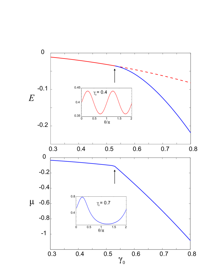
Figure 1 shows the energies and chemcial potentials of low-energy Bose condensate states by varying the parameter $\gamma_{0}$ for $d=2$. For small $\gamma_{0}$, the ground state is a symmetric state. As $\gamma_{0}$ is increased, a symmetry-breaking phase transition occurs at a critical value of $\gamma_{0}=0.528$. At this point, the symmetric state becomes dynamically unstable and the ground state changes to an asymmetric state. The ground state chemcial potential shows a kink at this critical point, wheras the ground state energy curve is smooth. This represents a second-order phase transition Qian . A similar behavior is also found in attractive BEC with unmodulated scattering length Kanamoto .

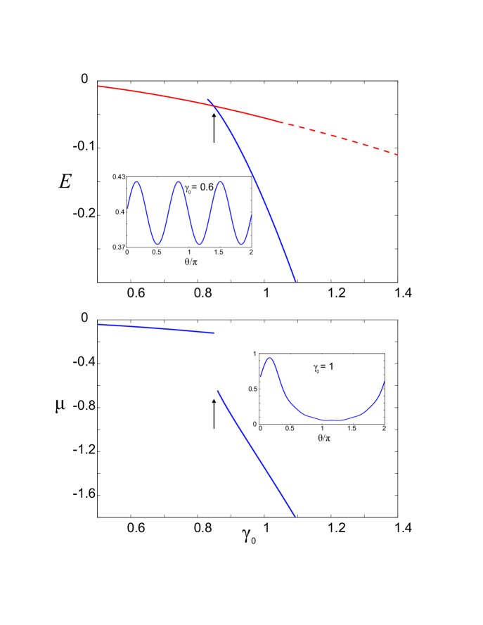
Next, we turn our attention to the case of $d=3$. The energies and chemical potentials as functions of $\gamma_{0}$ are plotted in Fig. 2. Similar to the $d=2$ case, for small $\gamma_{0}$, the ground state is symmetric. As $\gamma_{0}$ is increased, a symmetry-breaking phase transition occurs at a critical value of $\gamma_{0}=0.85$. However, unlike in the $d=2$ case, at this critical point, the symmetric state remains dynamically stable although the energy of the asymmetric state drops below that of the symmetric state. Furthermore, the ground state energy curve as a function of $\gamma_{0}$ shows a kink at this critical value, while the ground state chemical potential becomes discontinuous at this point. Therefore, the phase transition at this point is of first order. The dynamical instability of the symmetric state does not occur until $\gamma_{0}=1.04$.

To summarize our mean-field results, we have found that the nature of the phase transitions changes for different modulation period $d$ due to the presence of competing mechanisms in this system. When the modulation period $d=2$, the symmetry-breaking phase transition is of second order and is induced by dynamical instability of the associated states. For $d=3$, in contrast, the symmetric-breaking phase transition is of first order and is driven by the level crossing of different types of states. We have also investigated the cases for $d=4$ and 5 and found similar behavior as in $d=3$.

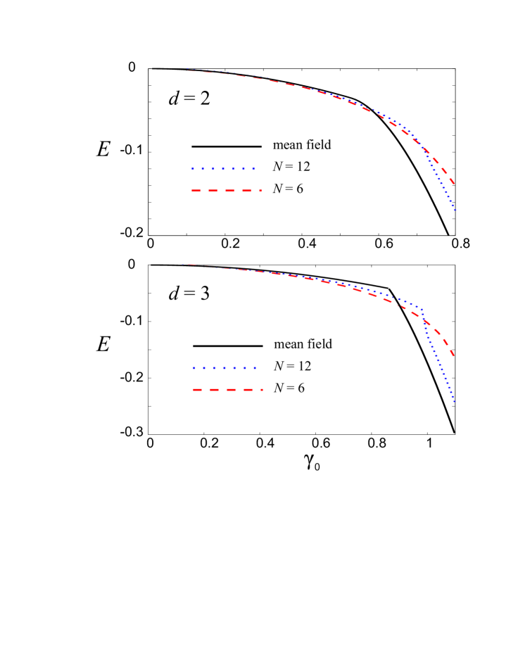
In Fig. 3, we plot the ground-state energy per atom of the many-body system as functions of $\gamma_{0}$ for the modulation period $d=2$ and $d=3$ . We see that the ground-state energy curve approaches the MFT result as $N$ increases, which is consistent with the usual quantum-semiclassical crossover behavior for finite-size quantum systems.

In the quantum mechanical treatment, unlike the mean field results, the spontaneous symmetry breaking of density distribution of ground state wavefunction in real space dose not occur. The density profile of the quantum mechanical ground state always matches the spatial modulation of the scattering length Qian . However, we can still gain important insights into the change in the characteristics of the wavefunctions by examining the quantum correlation which is neglected in the mean-field study.

For further discussion, we define the partial number operator between the interval $\theta\in[\varphi_{i},\varphi_{f}]$ as:

For the particular case of $d=3$, we define three partial particle number operators as follows:

Using these number operators, we can define the bipartite and tripartite correlation functions as:

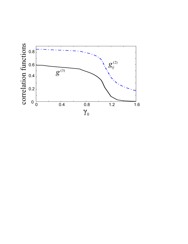
We plot the bipartite and tripartite correlations as functions of $\gamma_{0}$ in Fig. 4. All these correlations are monotonically decreasing functions of $\gamma_{0}$. In our calculation, the three two-body correlation functions $g_{12}^{(2)}$, $g_{13}^{(2)}$ and $g_{23}^{(2)}$ are essentially identical, which is also expected from the symmetry of the system. At $\gamma_{0}=0$, the ground state is exactly known: $\left|\Psi\right\rangle_{ground}=\frac{\left(a_{0}^{\dagger}\right)^{N}}{\sqrt{N!}}\left|{\rm vac}\right\rangle$. The theoretical values of bipartite and tripartite correlations can be obtained as:

which are in good agreement with the numerical results. When $N$ goes to infinity, all the bipartite and tripartite correlations approach unity at $\gamma_{0}=0$.

Figure 4 shows that although both bipartite and tripartite correlations decay as the interaction parameter $\gamma_{0}$ increases, the tirpartitle correlation $g^{\left(3\right)}$ decays into zero much faster than the bipartitle correlation $g_{ij}^{\left(2\right)}$. For the case of $N=6$ as illustrated in Fig. 4, $g^{\left(3\right)}$ is essentially zero at $\gamma_{0}=1.6$, while all the $g_{ij}^{\left(2\right)}$ are clearly non-zero at the same $\gamma_{0}$. This is reminiscent of the three-body entangled $W$-state, which can be written as

For the $W$-state, the tripartite entanglement characterized by the 3-tangle disappears and the bipartite entanglement characterized by concurrence remains finite Coffman . For large $\gamma_{0}$, our mean-field treatment presented earlier reveals that the ground state is characterized by asysmmetric state with three-fold degeneracy. Each of these degenerate mean-field state features a density peak at $\theta=(1+4i\pi)/6$ ($i=1,2,3$). In the quantum treatment, this degeneracy is lifted by quantum fluctuations, and the non-degenerate quantum ground state may be regarded as roughly a $W$-state formed by these three mean-field states.

Another important quantity to characterize the many-body state is the single-particle density matrix $\rho^{\left(1\right)}$ whose matrix element is defined as Penrose ; Leggett :

where the expectation value is calculated with respect to the ground state obtained using the TEBD method. Roughly speaking, $\rho_{ij}^{\left(1\right)}$ represents the probability amplitude of finding one particle at site $i$ and at the same time another particle at site $j$.

Because the matrix $\rho^{\left(1\right)}$ is Hermitian it can be diagonalized as:

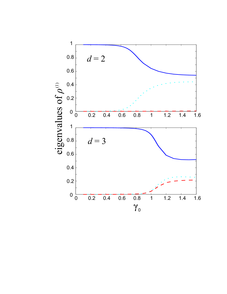
where the eigenvalues $p_{i}$ are non-negative and satisfy the constraint $\sum_{i}p_{i}=1$. For a bosonic system with $N\gg 1$, $p_{i}$ is closely related to the condensate fraction of the system. It is easy to see that, the system will be in a simple condensate state if and only if the largest eigenvaule is of order unity and all the other $p_{i}$’s are of order $O(N^{-1})$. If there are multiple $p_{i}$’s of order unity, the system is said to be in a fragmented condensate because all the corresponding states have appreciable occupation numbers. Finally, if all the $p_{i}$’s are of order $O(N^{-1})$, then the system is not Bose condensed. It is reasonable to speculate that, at small $N$, the condensate fraction versus the strength parameter $\gamma_{0}$ exhibits quantum crossover behavior. For $N=6$ with the modulation periods $d=2$ and $d=3$, we plot the three largest $p_{i}$’s versus $\gamma_{0}$ in Fig. 5. The figure shows that at small $\gamma_{0}$, the system may be characterized as a simple condensate. It becomes more and more fragmented as $\gamma_{0}$ is increased. In the large $\gamma_{0}$ limit, the eigenvalues approach some steady state values and there are $d$ eigenvalues which are much larger than the rest. This is consistent with the earlier argument that at large $\gamma_{0}$, the quantum many-body ground state can be roughly regarded as superpositions of the $d$-fold degenerate mean-field ground states.

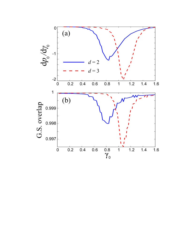
To further quantify the crossover from a simple condensate to a fragmented condensate, we adopt two methods as described below. In Fig. 6(a), we plot $dp_{0}/d\gamma_{0}$ as a function of $\gamma_{0}$, where $p_{0}$ is the largest single-particle density matrix eigenvalue. In Fig. 6(b), we plot the overlap of the ground-state wave function Zanardi $|\langle G(\gamma_{0})|G(\gamma_{0}+\delta\gamma)\rangle|$ for a small value of $\delta\gamma=0.02$, where $|G(\gamma_{0})\rangle$ denotes the ground state at $\gamma_{0}$. Both of these quantities measure how fast the characteristics of the ground state change as $\gamma_{0}$ is varied. These two measures provide consistent results: both exhibit a dip at some critical value $\gamma_{0}=0.84$ for $d=2$ and $\gamma_{0}=1.08$ for $d=3$, which we may define as the critical modulation depth where the system crosses from a simple condensate to a fragmented condensate.

Up to now, we have focused our attention on the static properties of the ground state. The low-energy excitations of the system in the vicinity of the crossover are also important because they expose fine characteristics valuable for understanding the system dynamics in the crossover. A powerful tool to study this is the time evolution of ground state survival probability Felker ; Wang . It describes the dynamical behavior of the system’s ground state under small perturbation in parameters in the system Hamiltonian. In our problem, we parameterize the Hamiltonian using the interaction strength modulation depth $\gamma_{0}$ such that $H=H(\gamma_{0})$. If $\gamma_{0}$ has a small variation $\delta\gamma$ so that $\gamma_{0}\rightarrow\gamma_{0}+\delta\gamma$, the ground state’s survival probablity is defined as

The survival probability can be considered as a special case of the quantum Loschmidt echo Peres . Incidentally, the numerical method we used to simulate our system, the TEBD algorithm, is very convenient in calculating the system’s time evolution and hence the survival probability.

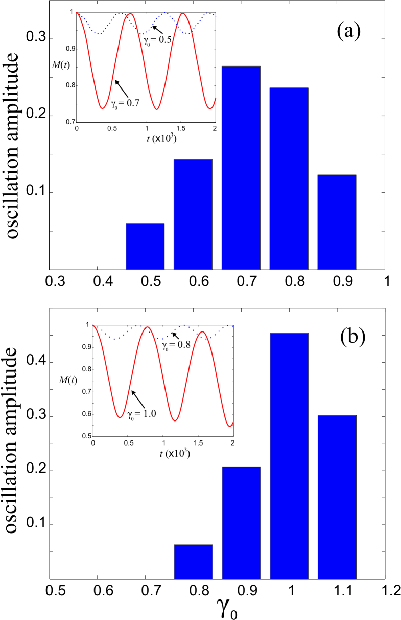
We calculated the ground state survival probability $M(t)$ and plot the results in Fig. 7 for $N=6$ and the perturbation in $\gamma_{0}$ is $\delta\gamma=0.1$. $M(t)$ exhibits roughly sinusoidal oscillations in time. The amplitude of the modulation reaches the maximum near critical points which are consistent with those found in previous static study and shown in Fig. 6. Indeed, the curve for the oscillation amplitude of the ground state’s survival probability can be used to predict the overlap between the perturbed and original ground state wave functions which is plotted in Fig. 6(b). The larger the oscillation amplitude in $M(t)$, the more sensitive the ground state wavefunction to the perturbation in the Hamiltonian.

References

- (1) I. Bloch, J. Dalibard, and W. Zwerger, Rev. Mod. Phys. 80, 885 (2008).
- (2) Yaroslav V. Kartashov, Boris A. Malomed, and Lluis Torner, arXiv:1010.2254, to appear in Rev. Mod. Phys.
- (3) Lisa C. Qian, Michael L. Wall, Shaoliang Zhang, Zhengwei Zhou, and Han Pu, Phys. Rev. A 77, 013611 (2008).
- (4) R. Kanamoto, H. Saito, and M. Ueda, Phys. Rev. A 67, 013608 (2003).
- (5) G. Vidal, Phys. Rev. Lett. 91, 147902 (2003); ibid, 93, 040502 (2004).
- (6) B. Schmidt, L. I. Plimak, and M. Fleischhauer, Phys. Rev. A 71, 041601(R) (2005); B. Schmidt, and M. Fleischhauer, Phys. Rev. A 75, 021601(R) (2007).
- (7) I. Danshita and P. Naidon, Phys. Rev. A 79, 043601 (2009).
- (8) See http://physics.mines.edu/downloads/software/tebd/
- (9) V. Coffman, J. Kundu, and W. K. Wootters, Phys. Rev. A 61, 052306 (2000).
- (10) O. Penrose and L. Onsager, Phys. Rev. 104, 576 (1956).
- (11) A. J. Leggett, Quantum Liquids, Oxford University Press (2006).
- (12) P. Zanardi and N. Paunkovi Phys. Rev. E 74, 031123 (2006).
- (13) P. Felker and A. Zewail, Adv. Chem. Phys. 70, 265 (1988).
- (14) W. G. Wang, P. Qin, L. He, and P. Wang, Phys. Rev. E 81, 016214 (2010).
- (15) A. Peres, Phys. Rev. A 30, 1610 (1984).
- (16) T. Mayteevarunyoo, B. A. Malomed, and G. Dong, Phys. Rev. A 78, 053601 (2008).
- (17) J. N. Milstein, The doctoral dissertation: ‘From Cooper Pairs to Molecules: Effective field theories for ultra-cold atomic gases near Feshbach resonances’ (University of Colorado), p118-120 (2004).