Quantum Phases of Time Order in Many-Body Ground States

We argue that ground state temporal properties of a quantum many-body system can be used to characterize or classify its phases. Hence, the concept of time order can be introduced analogous to an order parameter by bestowing it in the non-trivial temporal dependence. To exemplify the essence of the associated physics, we shall present an operational definition for time order and accordingly work out the exhaustive list of all allowed phases. According to the WO proposal Watanabe and Oshikawa (2015), a witness to CTC is the following two-time (or unequal time) auto-correlation function (with respect to ground state)

for operator $\hat{\Phi}(t)\equiv\int_{V}d^{D}x\hat{\phi}(\vec{x},t)$ defined as an integrated order parameter (over $D$-spatial-dimension), or analogously the volume averaged one,

with $\hat{\phi}(\vec{x},t)$ the corresponding local order parameter density operator $\hat{\phi}\equiv\hat{\Phi}/V$.

If $f(t)$ is time periodic, the system is in a state of CTC. This can be reformulated into an explicit operational protocol by introducing twisted vector. For a quantum many-body system with energy eigen-state $|\psi_{i}\rangle$, if there exists a coarse-grained Hermitian order parameter $\hat{\phi}$, $\hat{\phi}|\psi_{i}\rangle$ is called the eigen-state twisted vector; More generally, if $\hat{\phi}$ is non-Hermitian, $\hat{\phi}|\psi_{i}\rangle$ (or $\hat{\phi}^{\dagger}|\psi_{i}\rangle$) will be called the right (or left) eigen-state twisted vector.

The orthonormal set of eigen-wavefunctions $|\psi_{i}\rangle~{}(i=0,1,2,\cdots)$ for a system described by Hamiltonian $\hat{H}$ is arranged in increasing eigen-energies $\epsilon_{i}$ with $i=0$ denoting the ground state. When the coarse-grained order parameter $\hat{\phi}$ is Hermitian, the ground state twisted vector $|v\rangle$ can be expanded $|v\rangle\equiv\hat{\phi}(0)|\psi_{0}\rangle=\sum_{i=0}^{\infty}a_{i}|\psi_{i}\rangle$ into the eigen-basis. With the help of the Schrödinger equation $i{\partial|\psi(t)\rangle}/{\partial t}=\hat{H}|\psi(t)\rangle$ ($\hbar=1$ assumed throughout) for the system wave function $|\psi(t)\rangle$, we obtain

where $\eta_{j}\equiv|a_{j}|^{2}$ denote weights of the ground state twisted vector, $\eta_{0}$ the corresponding ground state weight, and $\eta_{j}$ (with $j>0$) the excited state weight.

When the coarse-grained order parameter $\hat{\phi}$ is non-Hermitian, we use $|v^{(l)}\rangle$ and $|v^{(r)}\rangle$ to denote respectively the left and right ground state twisted vectors and expand them analogously in the eigen-basis to arrive at $|v^{(l)}\rangle\equiv\hat{\phi}^{\dagger}|\psi_{0}\rangle=\sum_{i=0}^{\infty}b_{i}|\psi_{i}\rangle$ and $|v^{(r)}\rangle\equiv\hat{\phi}|\psi_{0}\rangle=\sum_{i=0}^{\infty}a_{i}|\psi_{i}\rangle$. In this case, we find

with $\eta_{j}\equiv b_{j}^{*}a_{j}$ weights of the ground state twisted vector instead. Similarly $\eta_{0}$ and $\eta_{j}$ ($j>0$) denote respectively ground and excited state weights.

Given an order parameter $\hat{\phi}$, quite generally $f(t)$ is a sum of many harmonic functions with amplitudes $\eta_{j}$ and characteristic frequencies $\omega_{j}\equiv\epsilon_{j}-\epsilon_{0}$. Nontrivial time dependence of the two-time auto-correlation function is thus imbedded in the energy spectra of $H$ as well as in the weights of the ground state twisted vector. For CTC order to exist, one of the excited state weights must be non-vanishing, or in rare cases, $f(t)$ can include harmonic terms of commensurate frequencies.

If $f(t)$ is a constant, the time dependence will be trivial. However, a subtlety appears when $f(t)$ is vanishingly small with respect to system size. Since what we are after is the system’s explicit temporal behavior or time dependence, which is easily washed out to $f(t)=0$ by a vanishing norm of the twisted vector. Such a difficulty can be mitigated by multiplying system volume $V$, i.e., using the twisted vector $|v\rangle\rightarrow V|v\rangle$ to check if the correlation for the bulk order parameter $F(t)\equiv V^{2}f(t)$ exhibits temporal dependence, or vanishes.

When $f(t)=0$ but $F(t)$ remains a periodic function, the system can still be considered a CTC. Such a remedy surprisingly captures the essence of generalized CTC of Ref.Medenjak et al. (2020).

The analysis presented above can be directly extended to excited states Syrwid et al. (2017). It is also straightforwardly applicable to non-Hermitian systems, as long as a plausible “ground state” can be identified, for example, by requiring its eigen-energy to possess the largest imaginary part or the smallest norm. Denoting the imaginary part of energy eigen-value $E_{i}$ as $\text{Im}(E_{i})$, a prefactor $\propto e^{\text{Im}(E_{i})t}$ then arises in the auto-correlation function, leading to unusual time functional order in the classification of time order.

Therefore, quantum many-body phases can be classified according to time order. The two-time auto-correlation function based complete operational procedure for classifying time order thus extends the definition of WO CTC in Ref. Watanabe and Oshikawa (2015). Our central results can be simply stated in the following: If $f(t)$ exhibits nontrivial time dependence, time order exists. If $f(t)=0$, but $F(t)$ displays nontrivial time dependence instead, generalized time order exists.

More specifically, if $f(t)={\rm const.}$ is nonzero, the system exhibits time trivial order. The same applies when $f(t)=0$ and $F(t)={\rm const.}$. For all other situations, nontrivial time order prevails. A complete classification for all time order ground state phases is shown in Table 1, according to the temporal behaviors of their auto-correlation functions $f(t)$ or $F(t)$. As shown in the Supplementary Material (SM), the above discussion and classification on time order can be extended to finite temperature systems as well.

The operational procedure outlined above presents a straightforward approach for detecting time order, albeit with reference to an order parameter operator. Hence more appropriately, this approach should be called order parameter assisted time order or symmetry-based (or -protected) time order, to emphasize its reference to symmetry order parameter of a quantum many-body system. The twisted vector facilitates easy calculations to distinguish between different time order phases from time trivial ones, as we illustrate below in terms of a few concrete examples. It is reasonable to expect that transitions between different time order phases can occur, reminiscent of phase transitions in the LGW spontaneous symmetry breaking paradigm.

A spin-1 atomic Bose-Einstein condensate (BEC) under single spatial mode approximation (SMA) Law et al. (1998); Pu et al. (1999); Yi et al. (2002) is described by the following Hamiltonian

where $\hat{a}_{m_{F}}(m_{F}=0,\pm 1)$ ($\hat{a}_{m_{F}}^{\dagger}$) denotes the annihilation (creation) operator for atom in the ground state Zeeman manifold $|F=1,m_{F}\rangle$ with corresponding number operator $\hat{N}_{m_{F}}=\hat{a}_{m_{F}}^{\dagger}\hat{a}_{m_{F}}$. The total atom number $\hat{N}=\hat{N}_{1}+\hat{N}_{0}+\hat{N}_{-1}$ is conserved. $p$ and $q$ are linear and quadratic Zeeman shifts that can be tuned independently Luo et al. (2017), while $c_{2}$ describes the strength of spin exchange interaction.

The validity of this model is well established based on extensive theoretical Chang et al. (2005); Zhang et al. (2010); Guzman et al. (2011); Xue et al. (2018) and experimental Chang et al. (2004); Anquez et al. (2016); Luo et al. (2017); Qiu et al. (2020) studies of spinor BEC over the years. The fractional population in spin states $|1,1\rangle$ and $|1,-1\rangle$, $\hat{n}_{\rm sum}\equiv N_{\rm sum}/{N}$, with $N_{\rm sum}={\hat{N}_{1}+\hat{N}_{-1}}=N-N_{0}$, is often chosen as an order parameter Damski and Zurek (2007); Lamacraft (2007); Anquez et al. (2016); Xue et al. (2018) with $N$ assuming the role of system size. The ground state twisted vector then becomes $|v\rangle\equiv\hat{n}_{\rm sum}|\psi_{0}\rangle$, and

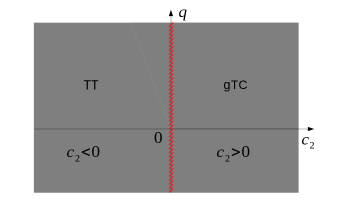
We will concentrate on the zero magnetization $F_{z}=0$ subspace and employ exact diagonalization (ED) to calculate eigen-states. $p=0$ is assumed since $F_{z}$ is conserved. Figure 1 illustrates the system’s complete time order phase diagram. For ferromagnetic interaction $c_{2}<0$ as with ${}^{87}\rm{Rb}$ atoms, the critical quadratic Zeeman shift $q/|c_{2}|=2$ splits the whole region into time trivial order (TT) phase for smaller $q$ that observes TTS, and generalized time crystalline (gTC) order phase for $q/|c_{2}|>2$ where TTS is spontaneously broken. The latter (gTC phase) is found to coincide with the polar phase Xue et al. (2018). Limited by available computation resources, the system sizes we explored with ED remain moderate which prevent us from mapping out the finer details in the immediate neighborhood of $q=2|c_{2}|$. Further elaboration of time order properties in this region is therefore needed. On the other hand, for antiferromagnetic interaction $c_{2}>0$ with ${}^{23}\rm{Na}$ atoms, we find $q=0$ separates TT phase from gTC order. We note here that $q=2|c_{2}|$ is the second-order quantum phase transition (QPT) critical point between the polar phase and the broken-axisymmetry phase of the ferromagnetic spin-1 BEC, while $q=0$ corresponds to the first-order QPT critical point for antiferromagnetic interaction .

More detailed discussions including the dependence of time order phases on system size, possible approaches to detect them, and extension to thermal state phases can be found in the SM.

As a second example, we consider time order phases of the quantum Rabi model described by the Hamiltonian

where $\hat{\sigma}_{x,z}$ is Pauli matrix of a two-level system (transition frequency $\Omega$), $\hat{a}(\hat{a}^{\dagger})$ is the annihilation (creation) operator for a single bosonic field mode (of frequency $\omega_{0}$), and $\lambda$ is their coupling strength.

It is known that the above model exhibits a QPT to a superradiant state, despite of its simplicity Hwang et al. (2015). The transition occurs at the critical point $g_{c}\equiv 1$, with the dimensionless parameter $g\equiv 2\lambda/\sqrt{\omega_{0}\Omega}$. The equivalent thermodynamic limit is approached by taking $\Omega/\omega_{0}\rightarrow\infty$. According to the studies in Ref. Hwang et al. (2015), an almost exact effective low-energy Hamiltonian for the normal phase ($g<1$) is given by

whose low-energy eigen-states are $|\phi_{\text{np}}^{m}(g)\rangle=\hat{\mathcal{S}}[r_{\text{np}}(g)]|m\rangle|\downarrow\rangle$ for $g\leq 1$, with $\hat{\mathcal{S}}[x]=\exp[{x}(\hat{a}^{\dagger 2}-\hat{a}^{2})/{2}]$ and $r_{\text{np}}(g)=-[\ln(1-g^{2})]/4$, and the energy eigen-values are $E_{\text{np}}^{m}(g)=m\epsilon_{\text{np}}(g)+E_{\text{G,np}}(g)$, with $\epsilon_{\text{np}}(g)=\omega_{0}\sqrt{1-g^{2}}$ and $E_{\text{G,np}}(g)=[{\epsilon_{\text{np}}(g)-\omega_{0}}]/{2}-{\Omega}/{2}$. For the supperadiant phase ($g>1$), the effective low energy Hamiltonian becomes

whose eigen-states are given by $|\phi_{\text{sp}}^{m}(g)\rangle_{\pm}=\hat{\mathcal{D}}[\pm\alpha_{g}]\hat{\mathcal{S}}[r_{\text{sp}}(g)]|m\rangle|\!\downarrow^{\pm}\rangle$, with $r_{\text{sp}}(g)=-[\ln(1-g^{-4})]/4$, $\alpha_{g}=\sqrt{(\Omega/4g^{2}\omega_{0})(g^{4}-1)}$, and $\hat{\mathcal{D}}[\alpha]=e^{\alpha(\hat{a}^{\dagger}-\hat{a})}$. The displacement-dependent spin states are $|\!\downarrow^{\pm}\rangle=\mp\sqrt{(1-g^{-2})/2}|\!\uparrow\rangle+\sqrt{(1+g^{-2})/2}|\!\downarrow\rangle$, while the energy eigen-values take the form $E_{\text{sp}}^{m}(g)=m\epsilon_{\text{sp}}(g)+E_{\text{G,sp}}(g)$, with $\epsilon_{\text{sp}}(g)=\omega_{0}\sqrt{1-g^{-4}}$ and $E_{\text{G,sp}}(g)=[{\epsilon_{\text{sp}}(g)-\omega_{0}}]/{2}-{\Omega}(g^{2}+g^{-2})/{4}$. More details can be found in the SM of Ref. Hwang et al. (2015).

For this model, the scaled average cavity photon number $\hat{n}_{c}={\omega_{0}}\hat{a}^{\dagger}\hat{a}/{\Omega}$ is a suitable order parameter with $\Omega/\omega_{0}$ assuming the role of system size. The corresponding bulk order parameter then becomes $\hat{N}_{c}=\hat{a}^{\dagger}\hat{a}$ or the average cavity photon number, and

For $g<1$, we find

respectively, where $\eta_{0}=\sinh^{4}(r_{\rm np})$ and $\eta_{2}=\cosh^{2}(r_{\rm np})\sinh^{2}(r_{\rm np})$. For $g>1$, we obtain

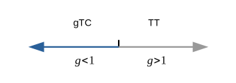
The time order phase diagram is shown in Fig. 2. When $g<1$, the system ground state corresponds to a generalized time crystalline order phase, while the system exhibits time trivial order when $g>1$. Despite of such a simple model composed of a two-level system and a bosonic field mode, the ground state of the quantum Rabi model displays intriguing temporal phase structure accompanied by a finite-component quantum phase transition.

Finally we consider two effective models with many-body spin-spin interaction and non-Hermitian effects. The first is described by Hamiltonian

with two $\sigma^{y}$ operators at sites $i$ and $j$ in a string of otherwise $\sigma^{x}$ $N$-body spin interaction. ${1}/[{N(N-1)}]$ is the normalization factor, $\lambda$ is the spin interaction strength, and $\gamma$ represents an effective dissipation rate. $\lambda>0$ and $\gamma\geq 0$ are both real numbers.

We observe that the Greenbergenr-Horne-Zeilinger (GHZ) states

correspond to two nondegenerate system eigen-states with eigen-energies $\pm(\lambda+\mathrm{i}\gamma)/2$. The spectra of this model system is bounded inside the circle of radius ${\sqrt{\lambda^{2}+\gamma^{2}}}/{2}$ in the complex plane. The eigen-state whose eigen-value has the largest imaginary part ia taken as the ground state, or $|{\rm GS}\rangle=|G_{+}\rangle$ with eigen-energy $\epsilon_{0}=(\lambda+\mathrm{i}\gamma)/2$. The highest excited state is $|G_{-}\rangle$, whose corresponding eigen-energy is $\epsilon_{2^{N}-1}=-(\lambda+\mathrm{i}\gamma)/2$.

An appropriate order parameter operator in this case becomes the average magnetization $\hat{m}=\sum_{i=1}^{N}\sigma_{i}^{z}/N$. The twisted vector becomes $|v\rangle=\hat{m}|{\rm GS}\rangle=|G_{-}\rangle$, and the auto-correlator can be easily worked out to be $f(t)=\lim_{N\rightarrow\infty}\langle\hat{m}(t)\hat{m}(0)\rangle=e^{-i\lambda t}e^{\gamma t}$. When $\gamma=0$, the system ground state exists time-crystalline order phase and corresponds to a continuous time crystal Kozin and Kyriienko (2019). When $\gamma\not=0$, the system exhibits time functional order, with an exploding $f(t)$ as time evolves.

A second non-Hermitian model Hamiltonian is given by

where $[\cdot]$ denotes the integer part, $\bm{\sigma}_{N+1}\equiv\bm{\sigma}_{1}$ corresponds to the periodic boundary condition, $\lambda$ and $\gamma$ are spin-string interaction strength and dissipation strength respectively as in the previous model, both of them are real. This Hamiltonian contains $[(N+1)/2]$-body interaction terms and supports GHZ state $|G_{+}\rangle$ as a non-degenerate excited state Facchi et al. (2011) with eigen-energy $\epsilon_{+}=-N$. The other two eigen-states of concern are $|\Psi^{(\pm)}\rangle\equiv({\alpha_{1}}|G_{-}\rangle+{\alpha_{2}}|\tilde{G}_{-,\mathcal{I}}\rangle)/{\sqrt{|\alpha_{1}|^{2}+|\alpha_{2}|^{2}}}$ with $\alpha_{1}=1$ and $\alpha_{2}={-(N+\epsilon^{(\pm)})}/{2(\lambda+\mathrm{i}\gamma)}$, where

The eigen-energies for $|\Psi^{(\pm)}\rangle$ are given by $\epsilon^{(\pm)}=-N+2\pm 2\sqrt{1+(\lambda+\mathrm{i}\gamma)^{2}}$, with more details of the derivation given in SM. For the same order parameter operator $\hat{m}$, we find $\hat{m}|\Psi_{0}\rangle\overset{N\rightarrow\infty}{\longrightarrow}{\alpha_{1}}|G_{+}\rangle/{\sqrt{|\alpha_{1}|^{2}+|\alpha_{2}|^{2}}}$.

At $\gamma=0$, the above non-Hermitian Hamiltonian (17) reduces to a Hermitian one, whose ground state $|\Psi_{0}\rangle$ corresponds to the one with smaller $\epsilon$ from $|\Psi^{(-)}\rangle$ and $|\Psi^{(+)}\rangle$, or $\epsilon_{0}=-N-2(\sqrt{1+\lambda^{2}}-1)$. The ground state $|\Psi_{0}\rangle$ for this non-Hermitian system is therefore chosen from $|\Psi^{(-)}\rangle$ or $|\Psi^{(+)}\rangle$ to be the one that deforms into the right Hermitian case one when $\gamma$ approaches zero. However, the criteria for the ground state energy $\epsilon_{0}$ corresponds to choosing the smaller one from $\epsilon^{(\pm)}$ when $\epsilon$ is real and choosing the one with the larger imaginary part when $\epsilon$ is complex.

Therefore we directly obtain

When $\lambda\not=0$ and $\gamma\not=0$, the system exists in time functional order phase, again results from the non-Hermitian Hamiltonian. When $\lambda\not=0$ but $\gamma=0$, the auto-correlation function reduces to

as for a genuine time crystal of the WO type exhibiting time crystalline order. When $\lambda=0$ and $0<|\gamma|\leq 1$, we find

The system ground state again exhibits time-crystalline order. When $\lambda=0$ and $|\gamma|>1$, we obtain

by choosing $\epsilon_{0}=-N+2+2\mathrm{i}\sqrt{\gamma^{2}-1}$ as the ground state eigen-energy from the two eigen-values $-N+2\pm 2\mathrm{i}\sqrt{\gamma^{2}-1}$. The system ground state now exhibits time functional order phase, with a decaying $f(t)$ as time evolves. When $\lambda=\gamma=0$,

the ground state reduces to time trivial order phase.

The above two non-Hermitian models represent direct generalizations of the Hermitian system considered in Refs. Kozin and Kyriienko (2019); Facchi et al. (2011). While slightly more complicated, they remain sufficient simple for compact analytical treatment, thus helping to reveal interesting and clear physical meanings of the underline time order.

According to the WO no-go theorem Watanabe and Oshikawa (2015), $f(t)$ for the ground state or the Gibbs ensemble of a general many-body Hamiltonian whose interactions are not-too-long ranged exhibits no temporal dependence, hence belongs to time trivial order according to our classification scheme. At first sight, this seems to sweep many important models of condensed matter physics into the same boring class of time trivial order phase. However, it remains to explore, for instance, many-body systems with more than two-body (or $k$-body) interactions, or non-Hermitian systems, which might support the existence of CTC. Inspired by the recent results on CTC Kozin and Kyriienko (2019), we believe more time crystalline phases will be uncovered and further understanding will be gained in the future.

As emphasized earlier, continuous time crystal results from spontaneously breaking continuous time translation symmetry. Due to the genuine time periodicity contained in CTC, it might be possible to explore and design new types of clocks based on macroscopic many-body systems, as the time period is directly related to energy spectra, and whose physical meaning is clearly the same as for atomic clock states. Furthermore, they are not affected by finite size effect in contrast to periodicity in DTC.

References

- Wen (2004) X.-G. Wen, Quantum Field Theory of Many-Body Systems (Oxford University Press, 2004).
- Fradkin (2004) E. Fradkin, Field Theories of Condensed Matter Physics , 2nd ed. (Oxford University Press, 2004).
- Sachdev (1999) S. Sachdev, Quantum Phase Transitions (Cambridge University Press, 1999).
- Landau and Lifshitz (1999) L. D. Landau and E. Lifshitz, Statistical Physics (Butterworth-Heinemann, 1999).
- Wilson and Kogut (1974) K. G. Wilson and J. Kogut, Physics reports 12, 75 (1974).
- Senthil et al. (2004) T. Senthil, A. Vishwanath, L. Balents, S. Sachdev, and M. P. Fisher, Science 303, 1490 (2004).
- Wen (1989) X. G. Wen, Phys. Rev. B 40, 7387 (1989).
- WEN (1990) X. G. WEN, International Journal of Modern Physics B 04, 239 (1990).
- Wen (2017) X.-G. Wen, Rev. Mod. Phys. 89, 041004 (2017).
- Wen (2019) X.-G. Wen, Science 363, eaal3099 (2019).
- Zeng and Wen (2015) B. Zeng and X.-G. Wen, Phys. Rev. B 91, 125121 (2015).
- Wen (2002) X.-G. Wen, Phys. Rev. B 65, 165113 (2002).
- Chen et al. (2015) X. Chen, F. J. Burnell, A. Vishwanath, and L. Fidkowski, Phys. Rev. X 5, 041013 (2015).
- Cheng et al. (2017) M. Cheng, Z.-C. Gu, S. Jiang, and Y. Qi, Phys. Rev. B 96, 115107 (2017).
- Heinrich et al. (2016) C. Heinrich, F. Burnell, L. Fidkowski, and M. Levin, Phys. Rev. B 94, 235136 (2016).
- Gu and Wen (2009) Z.-C. Gu and X.-G. Wen, Phys. Rev. B 80, 155131 (2009).
- Chen et al. (2011) X. Chen, Z.-X. Liu, and X.-G. Wen, Phys. Rev. B 84, 235141 (2011).
- Chen et al. (2013) X. Chen, Z.-C. Gu, Z.-X. Liu, and X.-G. Wen, Phys. Rev. B 87, 155114 (2013).
- Shirley et al. (2019) W. Shirley, K. Slagle, and X. Chen, SciPost Phys. 6, 15 (2019).
- Shirley et al. (2018) W. Shirley, K. Slagle, Z. Wang, and X. Chen, Phys. Rev. X 8, 031051 (2018).
- Vijay et al. (2016) S. Vijay, J. Haah, and L. Fu, Phys. Rev. B 94, 235157 (2016).
- Mierzejewski et al. (2017) M. Mierzejewski, K. Giergiel, and K. Sacha, Phys. Rev. B 96, 140201 (2017).
- Sacha (2015a) K. Sacha, Scientific reports 5, 10787 (2015a).
- Wilczek (2012) F. Wilczek, Phys. Rev. Lett. 109, 160401 (2012).
- Shapere and Wilczek (2012) A. Shapere and F. Wilczek, Phys. Rev. Lett. 109, 160402 (2012).
- Bruno (2013) P. Bruno, Phys. Rev. Lett. 111, 070402 (2013).
- Nozières (2013) P. Nozières, EPL (Europhysics Letters) 103, 57008 (2013).
- Watanabe and Oshikawa (2015) H. Watanabe and M. Oshikawa, Phys. Rev. Lett. 114, 251603 (2015).
- Sacha (2015b) K. Sacha, Phys. Rev. A 91, 033617 (2015b).
- von Keyserlingk et al. (2016) C. W. von Keyserlingk, V. Khemani, and S. L. Sondhi, Phys. Rev. B 94, 085112 (2016).
- Else et al. (2016) D. V. Else, B. Bauer, and C. Nayak, Phys. Rev. Lett. 117, 090402 (2016).
- Khemani et al. (2016) V. Khemani, A. Lazarides, R. Moessner, and S. L. Sondhi, Phys. Rev. Lett. 116, 250401 (2016).
- Yao et al. (2017) N. Y. Yao, A. C. Potter, I.-D. Potirniche, and A. Vishwanath, Phys. Rev. Lett. 118, 030401 (2017).
- Else et al. (2020) D. V. Else, C. Monroe, C. Nayak, and N. Y. Yao, Annual Review of Condensed Matter Physics 11, 467 (2020).
- Russomanno et al. (2017) A. Russomanno, F. Iemini, M. Dalmonte, and R. Fazio, Phys. Rev. B 95, 214307 (2017).
- Huang et al. (2018) B. Huang, Y.-H. Wu, and W. V. Liu, Phys. Rev. Lett. 120, 110603 (2018).
- Fan et al. (2020) C.-h. Fan, D. Rossini, H.-X. Zhang, J.-H. Wu, M. Artoni, and G. C. La Rocca, Phys. Rev. A 101, 013417 (2020).
- Machado et al. (2020) F. Machado, D. V. Else, G. D. Kahanamoku-Meyer, C. Nayak, and N. Y. Yao, Phys. Rev. X 10, 011043 (2020).
- Gong et al. (2018) Z. Gong, R. Hamazaki, and M. Ueda, Phys. Rev. Lett. 120, 040404 (2018).
- Gambetta et al. (2019) F. M. Gambetta, F. Carollo, M. Marcuzzi, J. P. Garrahan, and I. Lesanovsky, Phys. Rev. Lett. 122, 015701 (2019).
- Riera-Campeny et al. (2020) A. Riera-Campeny, M. Moreno-Cardoner, and A. Sanpera, Quantum 4, 270 (2020).
- Lazarides et al. (2020) A. Lazarides, S. Roy, F. Piazza, and R. Moessner, Phys. Rev. Research 2, 022002 (2020).
- Cosme et al. (2019) J. G. Cosme, J. Skulte, and L. Mathey, Phys. Rev. A 100, 053615 (2019).
- Zhang et al. (2017) J. Zhang, P. W. Hess, A. Kyprianidis, P. Becker, A. Lee, J. Smith, G. Pagano, I.-D. Potirniche, A. C. Potter, A. Vishwanath, N. Y. Yao, and C. Monroe, Nature (London) 543, 217 (2017).
- Choi et al. (2017) S. Choi, J. Choi, R. Landig, G. Kucsko, H. Zhou, J. Isoya, F. Jelezko, S. Onoda, H. Sumiya, V. Khemani, C. von Keyserlingk, N. Y. Yao, E. Demler, and M. D. Lukin, Nature (London) 543, 221 (2017).
- Rovny et al. (2018a) J. Rovny, R. L. Blum, and S. E. Barrett, Phys. Rev. B 97, 184301 (2018a).
- Rovny et al. (2018b) J. Rovny, R. L. Blum, and S. E. Barrett, Phys. Rev. Lett. 120, 180603 (2018b).
- Pal et al. (2018) S. Pal, N. Nishad, T. S. Mahesh, and G. J. Sreejith, Phys. Rev. Lett. 120, 180602 (2018).
- Autti et al. (2018) S. Autti, V. B. Eltsov, and G. E. Volovik, Phys. Rev. Lett. 120, 215301 (2018).
- Smits et al. (2018) J. Smits, L. Liao, H. T. C. Stoof, and P. van der Straten, Phys. Rev. Lett. 121, 185301 (2018).
- Cai et al. (2020) Z. Cai, Y. Huang, and W. V. Liu, Chinese Physics Letters 37, 050503 (2020).
- Kozin and Kyriienko (2019) V. K. Kozin and O. Kyriienko, Phys. Rev. Lett. 123, 210602 (2019).
- Medenjak et al. (2020) M. Medenjak, B. Buča, and D. Jaksch, Phys. Rev. B 102, 041117 (2020).
- Syrwid et al. (2017) A. Syrwid, J. Zakrzewski, and K. Sacha, Phys. Rev. Lett. 119, 250602 (2017).
- Law et al. (1998) C. K. Law, H. Pu, and N. P. Bigelow, Phys. Rev. Lett. 81, 5257 (1998).
- Pu et al. (1999) H. Pu, C. K. Law, S. Raghavan, J. H. Eberly, and N. P. Bigelow, Phys. Rev. A 60, 1463 (1999).
- Yi et al. (2002) S. Yi, O. E. Müstecaplıoğlu, C. P. Sun, and L. You, Phys. Rev. A 66, 011601 (2002).
- Luo et al. (2017) X.-Y. Luo, Y.-Q. Zou, L.-N. Wu, Q. Liu, M.-F. Han, M. K. Tey, and L. You, Science 355, 620 (2017).
- Chang et al. (2005) M.-S. Chang, Q. Qin, W. Zhang, L. You, and M. S. Chapman, Nat. Phys. 1, 111 (2005).
- Zhang et al. (2010) W. Zhang, B. Sun, M. Chapman, and L. You, Phys. Rev. A 81, 033602 (2010).
- Guzman et al. (2011) J. Guzman, G.-B. Jo, A. N. Wenz, K. W. Murch, C. K. Thomas, and D. M. Stamper-Kurn, Phys. Rev. A 84, 063625 (2011).
- Xue et al. (2018) M. Xue, S. Yin, and L. You, Phys. Rev. A 98, 013619 (2018).
- Chang et al. (2004) M.-S. Chang, C. Hamley, M. Barrett, J. Sauer, K. Fortier, W. Zhang, L. You, and M. Chapman, Phys. Rev. Lett. 92, 140403 (2004).
- Anquez et al. (2016) M. Anquez, B. A. Robbins, H. M. Bharath, M. Boguslawski, T. M. Hoang, and M. S. Chapman, Phys. Rev. Lett. 116, 155301 (2016).
- Qiu et al. (2020) L.-Y. Qiu, H.-Y. Liang, Y.-B. Yang, H.-X. Yang, T. Tian, Y. Xu, and L.-M. Duan, Science Advances 6, eaba7292 (2020).
- Damski and Zurek (2007) B. Damski and W. H. Zurek, Phys. Rev. Lett. 99, 130402 (2007).
- Lamacraft (2007) A. Lamacraft, Phys. Rev. Lett. 98, 160404 (2007).
- Hwang et al. (2015) M.-J. Hwang, R. Puebla, and M. B. Plenio, Phys. Rev. Lett. 115, 180404 (2015).
- Facchi et al. (2011) P. Facchi, G. Florio, S. Pascazio, and F. V. Pepe, Phys. Rev. Lett. 107, 260502 (2011).