Quantum Pricing with a Smile: Implementation of Local Volatility Model on Quantum Computer

We first present the calculation flow in the PRN-on-a-register way. We consider the flow until calculation of the sum of payoffs, which corresponds to from the first to the third line in (13), since the controlled rotation in the fourth line does not depend on the problem.

In the PRN-on-a-register way, PRNs are used for evolution of the asset price (10). More concretely, we preselect some sequence of pseudo standard normal random numbers (PSNRNs) and divide it into subsequences, then evolve the asset price using them.

Before we present the calculation flow, we explain some setups. We prepare the following register:

• •

  $R_{\rm samp}$

  This is a register where a superposition of integers which determine the start point of the PSNRN sequence. We write its qubit number as $n_{\rm samp}$. $N_{\rm samp}=2^{n_{\rm samp}}$ is the number of sample paths we generate.

• •

  $R_{W}$

  This is a register where we sequentially generate PSNRNs.

• •

  $R_{S}$

  This is a register where the value of the asset price is stored and which we update for each time step of the evolution, using $R_{W}$.

• •

  $R_{\rm payoff}$

  This is a register into which the payoffs determined by $R_{S}$ are added.

Note that we need some ancillary registers in addition to the above registers. We assume that the required calculation precision is $n_{\rm dig}$-bit accuracy and $R_{W},R_{S},R_{\rm payoff}$ and ancillary registers necessary to update them have $n_{\rm dig}$ qubits.

We assume that the following gates are available to generate a sequence of PSNRNs.

• •

  $P_{W}$

  This progresses a PSNRN sequence by one step. In other words, it acts on $R_{W}$ and updates $x_{i}$ to $x_{i+1}$, where $x_{i}$ is the $i$-th element of the sequence: $\ket{x_{i}}\rightarrow\ket{x_{i+1}}$.

• •

  $J_{W}$

  This lets the PSNRN sequence jump to the starting point. That is, it is input an integer $i$ on a register and outputs $x_{in_{t}+1}$ into another register which is initially set to $\ket{0}$: $\ket{i}\ket{0}\rightarrow\ket{i}\ket{x_{in_{t}+1}}$. Remember that $n_{t}$, the number of time steps, is equal to the number of RNs used to generate one sample path.

The concrete implementation of these gates are discussed later.

Then, the calculation flow is as follows:

1. 1.

   Initialize all registers to $\ket{0}$ except $R_{S}$, which is initialized to $\ket{S_{t_{0}}}$.

2. 2.

   Generate a equiprobable superposition of $\ket{0},\ket{1},...,\ket{N_{\rm{samp}}-1}$, that is, $\frac{1}{\sqrt{N_{\rm{samp}}}}\sum_{i=0}^{N_{\rm{samp}}-1}{\ket{i}_{n_{\rm{PRN}}}}$ on $R_{\rm samp}$. This is done by operating a Hadamard gate to each of $n_{\rm{samp}}$ qubits.

3. 3.

   Operate $J_{W}$ to set $x_{in_{t}+1}$ to $R_{W}$, where $i$ is determined by the state of $R_{\rm{samp}}$. These are the starting points of subsequences.

4. 4.

   Perform the time evolution (10) using the value on $R_{W}$. $R_{S}$ is updated from $\ket{S_{t_{0}}}$ to $\ket{S_{t_{1}}}$.

5. 5.

   Calculate the payoff at time $t_{1}$ and add into $R_{\rm payoff}$.

6. 6.

   Operate $P_{\rm{PRN}}$ to update $R_{W}$ from $x_{in_{t}+1}$ to $x_{in_{t}+2}$.

7. 7.

   Iterate operations similar to 4-6 for each time steps until the time reaches $t_{n_{t}}$.

8. 8.

   Finally we obtain a superposition of states in which the value on $R_{\rm payoff}$ is the sum of payoffs in each sample path. Estimate the expectation value of $R_{\rm payoff}$ by methods like Bassard ; Suzuki . This is an estimate for (12).

Here and hereafter, we assume that a payoff arises at each time step, for simplicity.

The flow of state transformation is as follows:

		$\displaystyle\ket{0}\ket{0}\ket{S_{t_{0}}}\ket{0}$
	$\displaystyle\xrightarrow{2}$	$\displaystyle\frac{1}{\sqrt{N_{\rm{samp}}}}\sum_{i=0}^{N_{\rm{samp}}-1}$	$\displaystyle{\ket{i}}\ket{0}\ket{S_{t_{0}}}\ket{0}$
	$\displaystyle\xrightarrow{3}$	$\displaystyle\frac{1}{\sqrt{N_{\rm{samp}}}}\sum_{i=0}^{N_{\rm{samp}}-1}$	$\displaystyle{\ket{i}}\ket{x_{in_{t}+1}}\ket{S_{t_{0}}}\ket{0}$
	$\displaystyle\xrightarrow{4}$	$\displaystyle\frac{1}{\sqrt{N_{\rm{samp}}}}\sum_{i=0}^{N_{\rm{samp}}-1}$	$\displaystyle{\ket{i}}\ket{x_{in_{t}+1}}\ket{S^{(i)}_{t_{1}}}\ket{0}$
	$\displaystyle\xrightarrow{5}$	$\displaystyle\frac{1}{\sqrt{N_{\rm{samp}}}}\sum_{i=0}^{N_{\rm{samp}}-1}$	$\displaystyle{\ket{i}}\ket{x_{in_{t}+1}}\ket{S^{(i)}_{t_{1}}}\ket{\sum_{j=1}^{1}{f^{\rm pay}_{j}(S^{(i)}_{t_{j}})}}$
	$\displaystyle\xrightarrow{6}$	$\displaystyle\frac{1}{\sqrt{N_{\rm{samp}}}}\sum_{i=0}^{N_{\rm{samp}}-1}$	$\displaystyle{\ket{i}}\ket{x_{in_{t}+2}}\ket{S^{(i)}_{t_{1}}}\ket{\sum_{j=1}^{1}{f^{\rm pay}_{j}(S^{(i)}_{t_{j}})}}$
	$\displaystyle\xrightarrow{7}$	$\displaystyle...\qquad\quad\quad\quad$
	$\displaystyle\xrightarrow{7}$	$\displaystyle\frac{1}{\sqrt{N_{\rm{\rm{samp}}}}}\sum_{i=0}^{N_{\rm{\rm{samp}}}-1}$	$\displaystyle{\ket{i}}\ket{x_{in_{t}+n_{t}}}\ket{S^{(i)}_{t_{n_{t}}}}\ket{\sum_{j=1}^{n_{t}}{f^{\rm pay}_{j}(S^{(i)}_{t_{j}})}},$		(15)

where the first, second, third and fourth kets correspond to $R_{\rm samp},R_{W},R_{S}$ and $R_{\rm payoff}$, respectively.

Schematically, the circuit which realizes the flow (15) is as shown in Figure 1. In the figure, the gate $U_{j}$ corresponds to the $j$-th step of asset price evolution, that is, the $j$-th iteration of step 4-6 in the above calculation flow.

$U_{j}$ is implemented as shown in Figure 2. $P_{W}$ is already explained and the gate ${\rm Payoff}_{j}$ calculates $f^{\rm pay}_{j}(S^{(i)}_{t_{j}})$ using $R_{S}$ and adds it into $R_{\rm payoff}$. In addition to these, $U_{j}$ has gates $V^{(j)}_{1},...,V^{(j)}_{n_{S}}$, which update $R_{S}$.

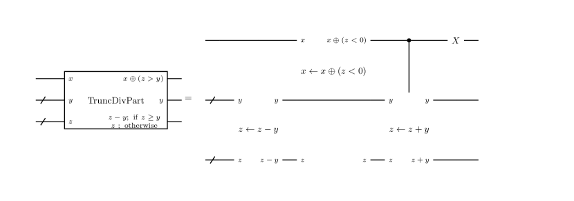
The detail of $V^{(j)}_{k}$ is shown in Figure 3. This gate (i) checks whether the asset price is in the $k$-th interval $[s_{j,k-1},s_{j,k})$, (ii) if so, update $R_{S}$ using the LV in the interval, (iii) clears the intermediate output. It requires ancillary registers $R_{\rm count},R_{S^{\prime}}$ and $R_{g}$. They have $\lceil\log_{2}{n_{t}}\rceil,n_{\rm dig}$ and 1 qubits respectively. At the start of $V^{(j)}_{k}$, $R_{\rm count}$ takes $\ket{j}$ or $\ket{j+1}$ and the others take $\ket{0}$. Then the detailed calculation flow is:

1. 1.

   If $R_{\rm count}$ is $j$ and $R_{S}$ is in $[s_{j,k-1},s_{j,k})$, flip $R_{g}$.

2. 2.

   If $R_{g}$ is 1, update $R_{S}$ as

   $$S_{t_{j}}\rightarrow S_{t_{j+1}}=S_{t_{j}}+(a_{j,k}S_{t_{j}}+b_{j,k})\sqrt{\Delta t_{j}}x_{in_{t}+j}$$

   (16)

   using the value $x_{in_{t}+j}$ on $R_{W}$ and add 1 to $R_{\rm count}$.

3. 3.

   Calculate

   $$\frac{S_{t_{j+1}}-b_{j,k}\sqrt{\Delta t_{j}}x_{in_{t}+j}}{1+a_{j,k}\sqrt{\Delta t_{j}}x_{in_{t}+j}}$$

   (17)

   into $R_{S^{\prime}}$, using the value on $R_{S}$ as $S_{t_{j+1}}$ and that on $R_{W}$ as $x_{in_{t}+j}$.

4. 4.

   If $R_{\rm count}$ is $j+1$ and $R_{S^{\prime}}$ is in $[s_{j,k-1},s_{j,k})$, flip $R_{g}$. This uncomputes $R_{g}$.

5. 5.

   Do the inverse operation of 3.

Let us explain the meaning of this flow. First, $R_{\rm count}$ is necessary as an indicator of whether the $j$-th step of evolution has been already done or not. Without this, it is possible that the asset price is doubly updated in a time step. If and only if the $j$-th step has not been done, that is, $R_{\rm count}$ is $j$ and the asset price is in $[s_{j,k-1},s_{j,k})$, the update of the asset price with the LV function $a_{j,k}S+b_{j,k}$ is done. To do this conditional update, the check result is intermediately output to $R_{g}$ and the gate corresponding (16) is operated on $R_{S}$ under control by $R_{g}$. Besides, the increment of $R_{\rm count}$ controlled by $R_{g}$ is also done, so that $R_{\rm count}$ indicates completion of the $j$-th step if so. Steps 3-5 is necessary to clear $R_{g}$. If the asset price has been updated in Step 2, Step 3 draws back it to the value before the update. Conversely, we can determine whether the update has been done in Step 2 from the result of Step 3. That is, for the reason mentioned soon later, the condition that $R_{\rm count}$ is $j+1$ and $R_{S^{\prime}}$ is in $[s_{j,k-1},s_{j,k})$ after Step 3 is equivalent to the condition that $R_{\rm count}$ is $j$ and $R_{S}$ is in $[s_{j,k-1},s_{j,k})$ before Step 2. Therefore, Step 4 flip $R_{g}$ if and only if it is $\ket{1}$, so it goes back to $\ket{0}$. In summary, through the sequential operation of $V^{(j)}_{1},...,V^{(j)}_{n_{S}+1}$, $R_{S}$ is updated only once at the appropriate $V^{(j)}_{k}$, $R_{\rm count}$ is updated from $\ket{j}$ to $\ket{j+1}$ and all intermediate outputs on ancillary registers are cleared.

We here mention a restriction on the LV model so that it can be implemented in the PRN-on-a-register way. Note that through $V^{(j)}_{1},...,V^{(j)}_{n_{S}+1}$, the state is transformed from $\ket{j}\ket{S^{(i)}_{t_{j}}}$ to $\ket{j+1}\ket{S^{(i)}_{t_{j+1}}}$, where the first and second kets correspond to $R_{\rm count}$ and $R_{S}$ respectively and other registers are omitted since they are unchanged. This means that the map from $S^{(i)}_{t_{j}}$ to $S^{(i)}_{t_{j+1}}$ must be one-to-one correspondence, since unitarity is violated if not. Actually, this is not so strong restriction. As shown in Appendix, if we set $a_{i,j},b_{i,j}$ so that $\sigma(t,S)$ is continuous with respect to $S$ and we set $\Delta t_{j}$ is small enough that the increment $\Delta S_{t_{j}}$ is much smaller than $S_{t_{j}}$ itself, the above condition is satisfied.

This one-to-one correspondence lets Step 3 work. That is, since the map between $S^{(i)}_{t_{j}}$ and $S^{(i)}_{t_{j+1}}$ is one-to-one correspondence, the result of Step 3 is in $[s_{j,k-1},s_{j,k})$ if and only if the value on $R_{S}$ before Step 3 is in the image of $[s_{j,k-1},s_{j,k})$ under the map.

We now consider how to implement respective gates in the PRN-on-a-register way to the level of four arithmetic operations.

Note that most parts of $V^{(j)}_{k}$ consist of only arithmetic operations, addition, subtraction, multiplication, division and comparison, which mentioned in Sec IV.1.

For example, the gate $z\leftarrow z\oplus(x=j\ {\rm and}\ y\in I)$ can be divided to two parts. The first part is checking that the value on $R_{\rm count}$ is equal to $j$ and this can be done by the multiple control Toffoli gate, which is studied in Selinger ; Amy ; Maslov . The second part is checking that the asset price is in a given interval, which can be constructed from two comparisons. Combining these, the gate $z\leftarrow z\oplus(x=j\ {\rm and}\ y\in I)$ in Figure 3 is constructed as shown in Figure 4. Note that the bitwise flips $X^{1-j_{0}}\otimes...\otimes X^{1-j_{n_{x}-1}}$ are operated before the multi control Toffoli. Here, $j_{a}$ is the $a$-th digit of the binary representation of $j$, so the $a$-th qubit is flipped if and only if $j_{a}=0$. This convert $\ket{x}$ to $\ket{1}...\ket{1}$ if and only if $x=j$.

The operation $x\leftarrow x+(ax+b)y$ in Figure 3 can be realized as follows:

	$\displaystyle\ket{x}\ket{y}\ket{0}$	$\displaystyle\rightarrow$	$\displaystyle\ket{x}\ket{y}\ket{1}$		(18)
		$\displaystyle\rightarrow$	$\displaystyle\ket{x}\ket{y}\ket{1+ay}$
		$\displaystyle\rightarrow$	$\displaystyle\ket{(1+ay)x}\ket{y}\ket{1+ay}$
		$\displaystyle\rightarrow$	$\displaystyle\ket{(1+ay)x+by}\ket{y}\ket{1+ay}$
		$\displaystyle\rightarrow$	$\displaystyle\ket{(1+ay)x+by}\ket{y}\ket{0},$

where the third ket corresponds to an ancillary register. The first arrow is just setting a constant on a register. The second arrow is the multiplication by a constant $a$. The third arrow is the self-update multiplication, so it needs another ancillary register. The fourth arrow is again multiplication by a constant $b$ and the final arrow is uncomputation of the first and second arrows. Note that this is done under control by $R_{g}$. In order for this to be controlled, it is sufficient to control only the second, fourth and final arrows, since the third arrow becomes a multiplication by 1 without the second. Also note that multiplication by a $n$-bit constant $a$ or $b$ can be done by $n$ adders, that is, $n$ shift-and-add’s: $ax=\sum_{i=0}^{n-1}{a_{i}2^{i}x}$, where $a_{i}$ is the $i$-th bit of $a$. This saves qubits compared with the case where we use a multiplier, which needs holding $a$ on an ancillary register.

The operation $x\leftarrow(x-by)/(1+ay)$ in Figure 3 is done as follows:

	$\displaystyle\ket{x}\ket{y}\ket{0}\ket{0}$	$\displaystyle\rightarrow$	$\displaystyle\ket{x}\ket{y}\ket{1}\ket{0}$		(19)
		$\displaystyle\rightarrow$	$\displaystyle\ket{x}\ket{y}\ket{1+ay}\ket{0}$
		$\displaystyle\rightarrow$	$\displaystyle\ket{x-by}\ket{y}\ket{1+ay}\ket{0}$
		$\displaystyle\rightarrow$	$\displaystyle\ket{x-by}\ket{y}\ket{1+ay}\ket{(x-by)/(1+ay)},$

where the first, second, third and fourth kets are $R_{S},R_{W}$, another ancillary register and $R_{S^{\prime}}$, respectively. Here, the first and second arrows are same as (18), the third is the multiplication by a constant $-b$ and the final one is division. Here, we do not have to uncompute $R_{S}$ and the ancillary register, since the whole of this operation is uncomputed soon later in $V_{j,k}$.

In Miyamoto , implementation of PRN on quantum circuits is presented, using the PRN generator called PCGPCG . Note that this PRN generator generates uniform RNs. We now need PSNRNs, so we must transform uniform distribution to standard normal distribution. There are some method and we adopt the inverse transform sampling. Schematically, $J_{W}$ and $P_{W}$ are implemented as shown in Figure 5. Here, $J_{PRN}$ is the gate to let the PRN sequence jump to the $in_{t}+1$ and $P_{PRN}$ is the gate to progress the PRN sequence by a step. They sequentially generate uniform RNs on the ancillary register $R_{\rm PRN}$ and they are transformed to PSNRN on $R_{W}$.

Although we refer to Miyamoto for the detail of implementation of the PRN generator, we here briefly explain. This generator is combination of linear congruential generator (LCG) and permutation of bit string. For LCG, update of the PRN sequence is done by

$$x_{n+1}=ax_{n}+c\ {\rm mod}\ N,$$

(20)

where $a,N$ are positive integers and $c$ is a nonnegative integer, and the $n$-th element of the sequence is computed from $n$ and the initial value $x_{0}$ by

$$x_{n}=a^{n}x_{0}+\frac{c(a^{n}-1)}{a-1}\ {\rm mod}\ N,.$$

(21)

According to Vedral , we can construct the modular adder using 5 plain adders. Modular multiplication by a $n$-bit constant can be done as $n$ modular shift-and-add’s. Modular division by a constant $a-1$ can be done as modular multiplication by a constant integer $\beta$ such that $\beta(a-1)=1\ {\rm mod}\ N$, if exists. Modular exponentiation $a^{x}\ {\rm mod}\ N$ is computed as a sequence controlled modular multiplicationVedral . So, to summarize, we can perform (20) and (21) using only controlled adders. In (20), the state is transformed as

	$\displaystyle\ket{x}\ket{0}\ket{0}$	$\displaystyle\rightarrow$	$\displaystyle\ket{x}\ket{ax\ {\rm mod}\ N}\ket{0}$		(22)
		$\displaystyle\rightarrow$	$\displaystyle\ket{0}\ket{ax\ {\rm mod}\ N}\ket{0}$
		$\displaystyle\rightarrow$	$\displaystyle\ket{0}\ket{ax\ {\rm mod}\ N}\ket{c}$
		$\displaystyle\rightarrow$	$\displaystyle\ket{0}\ket{ax+c\ {\rm mod}\ N}\ket{c}$
		$\displaystyle\rightarrow$	$\displaystyle\ket{0}\ket{ax+c\ {\rm mod}\ N}\ket{0}.$

In the circuit we are considering, the first and second registers are $R_{\rm PRN}$ and an ancillary register, which interchange their role at every step, and the third is another ancillary register. Each step corresponds to an elementary operation as follows. The first arrow is modular multiplication. The second arrow is the inverse modular multiplication by a integer $\alpha$ such that $a\alpha=1\ {\rm mod}\ N$ and this clearing step is necessary to avoid increase of ancillas. The third is just loading $c$ on an ancillary register, the fourth is modular addition and the last is unloading. (21) progresses as follows:

			$\displaystyle\ket{n}\ket{0}\ket{0}\ket{0}$		(23)
		$\displaystyle\rightarrow$	$\displaystyle\ket{n}\ket{a^{n}\ {\rm mod}\ N}\ket{0}\ket{0}$
		$\displaystyle\rightarrow$	$\displaystyle\ket{n}\ket{a^{n}\ {\rm mod}\ N}\ket{\left(x_{0}+\frac{c}{a-1}\right)a^{n}\ {\rm mod}\ N}\ket{0}$
		$\displaystyle\rightarrow$	$\displaystyle\ket{n}\ket{a^{n}\ {\rm mod}\ N}\ket{\left(x_{0}+\frac{c}{a-1}\right)a^{n}\ {\rm mod}\ N}\ket{\frac{c}{a-1}}$
		$\displaystyle\rightarrow$	$\displaystyle\ket{n}\ket{a^{n}\ {\rm mod}\ N}\ket{\left(x_{0}+\frac{c}{a-1}\right)a^{n}-\frac{c}{a-1}\ {\rm mod}\ N}\ket{\frac{c}{a-1}}$
		$\displaystyle\rightarrow$	$\displaystyle\ket{n}\ket{0}\ket{\left(x_{0}+\frac{c}{a-1}\right)a^{n}-\frac{c}{a-1}\ {\rm mod}\ N}\ket{0},$

where the first, third, second and fourth registers are respectively $R_{\rm samp},R_{\rm PRN}$ and two ancillary registers. The first arrow is modular exponentiation, the second is modular multiplication, the third is loading, the fourth is modular addition and the last is uncomputation of the first and third.

We do not explain permutation: see Miyamoto for the detail. We just make a comment that it is implemented by a simple circuit, for example, Xorshift is implemented as a sequence of CNOT.

We also need the gate to calculate $\Phi_{\rm SN}^{-1}$, the inverse function of CDF of standard normal distribution. There are some ways to calculate this efficiently and we here adopt the method in Hormann . In the method, $\mathbb{R}$ is divided into some intervals and $\Phi_{\rm SN}^{-1}$ is approximated by a polynomial in each interval. We adopt the setting where the number of intervals is 109⁶⁶6if we include $(-\infty,x^{\rm ICDF}_{0})$ and $[x^{\rm ICDF}_{n^{\rm ICDF}},\infty,)$, it is 111 and polynomials are cubic, which realizes the error smaller than $10^{-6}$. Here, we write the approximated inverse CDF as

$$\Phi_{\rm SN}^{-1}(x)\approx c_{m,3}x^{3}+c_{m,2}x^{2}+c_{m,1}x+c_{m,0}$$

(24)

for $x^{\rm ICDF}_{m-1}\leq x<x^{\rm ICDF}_{m},m=0,1,...,n_{\rm ICDF}+1$, where $x^{\rm ICDF}_{0}<x^{\rm ICDF}_{1}<...<x^{\rm ICDF}_{n_{\rm ICDF}}$ are the end points of the intervals and $n_{\rm ICDF}$ is the number of the interval. Consider that $x^{\rm ICDF}_{-1}=-\infty,x^{\rm ICDF}_{n_{\rm ICDF}+1}=+\infty$.

Such a piecewise cubic function can be implemented as Figure 6. We here explain how it works. First, the sequence of comparators and “Load $c_{m,i}^{\prime}s$” gates load $c_{m,0},...,c_{m,3}$ into the register $R_{c_{0}},...,R_{c,3}$ respectively as follows. The comparators compare the value $x$ of $R_{\rm PRN}$ and the grid points $x^{\rm ICDF}_{m}$ and flip $R_{g}$ if $x<x^{\rm ICDF}_{m}$. If $R_{g}$ is 1, the “Load $c_{m,i}^{\prime}s$” gates are activated. They are actually collections of bitwise flips, that is, $X$ gates. If $x\geq x^{\rm ICDF}_{n_{\rm ICDF}}$, only “Load $c_{n_{\rm ICDF}+1,i}^{\prime}s$” gate is performed and it loads $c_{n_{\rm ICDF}+1,0},...,c_{n_{\rm ICDF}+1,3}$. If $x^{\rm ICDF}_{n_{\rm ICDF}-1}\leq x<x^{\rm ICDF}_{n_{\rm ICDF}}$, “Load $c_{n_{\rm ICDF},i}^{\prime}s$” and “Load $c_{n_{\rm ICDF}+1,i}^{\prime}s$” are performed. So, we set “Load $c_{n_{\rm ICDF},i}^{\prime}s$” so that it compensates flips done by “Load $c_{n_{\rm ICDF}+1,i}^{\prime}s$” and $c_{n_{\rm ICDF},0},...,c_{n_{\rm ICDF},3}$ are successfully loaded. The case where $x$ is in another interval is similar. The point is that if $x^{\rm ICDF}_{M-1}\leq x<x^{\rm ICDF}_{M}$, every other gates are activated. That is, the activated gates are “Load $c_{m,i}^{\prime}s$” of $m=M,M+2,...,n_{\rm ICDF},n_{\rm ICDF}+1$ if $n_{\rm ICDF}-M$ is even and $m=M,M+2,...,n_{\rm ICDF}-1,n_{\rm ICDF}+1$ if $n_{\rm ICDF}-M$ is odd. This is because every comparator after the $M$-th one flips $R_{g}$ and $R_{g}$ takes 0 and 1 alternatingly. Considering this, the $X$ gates in “Load $c_{m,i}^{\prime}s$” are set as Figure 7, so that $c_{m,0},...,c_{m,3}$ for appropriate $m$ are loaded after the sequence of all activated gates. After load of coefficients, the cubic function is calculated in the Horner’s method

$$((c_{m,3}x+c_{m,2})x+c_{m,1})x+c_{m,0}.$$

(25)

This is done by the sequence of adders and multipliers in the latter half of the circuit in Figure 6.

In this paper, we do not consider gates to calculate payoffs in detail, since the resource the gates require is same in both the PRN-on-a-register way and the register-per-RN way. We here make just a short comment. In many cases, a payoff can be expressed in the following form:

$$f^{\rm pay}_{i}=\min\{\max\{a_{i}S_{t_{i}}+b_{i},f_{i}\},c_{i}\},$$

(26)

where $a_{i},b_{i},c_{i},f_{i}$ are real constants, that is, a linear function of the asset price with the upper bound (cap) $c_{i}$ and the lower bound (floor) $f_{i}$. For example, a payoff in an European call option (1) corresponds to $a_{i}=1,b_{i}=-K,c_{i}=+\infty,f_{i}=0$. Payoffs expressed as (26) can be calculated easily by combination of comparators, adders and multipliers.

Also for the register-per-RN way, we start from presenting the calculation flow, which is somewhat simpler than the PRN-on-a-register way. Again, we consider the flow until calculation of the payoff sum.

Before we present the calculation flow, we explain the required registers.

• •

  $R_{W_{i}},i=1,...,n_{t}$

  This is a register for the $i$-th SNRN. We need such a register per random number, so the total number is $n_{t}$.

• •

  $R_{S_{i}},i=0,1,...,n_{t}$

  This is a register where the value of the asset price at time $t_{i}$ is held.

• •

  $R_{{\rm payoff},i},i=1,...,n_{t}$

  This is a register where the value of the sum of payoffs by $t_{i}$ is held.

We again omit ancillary registers here and explain them later. Besides, we again assume that these and ancillary registers necessary to update them have $n_{\rm dig}$ qubits.

We here concretely define a superposition of SNRN values as the following state. In advance, we set the equally spaced $N_{\rm SN}+1$ points for discretization of the distribution $x_{{\rm SN},0}<x_{{\rm SN},1}<...<x_{{\rm SN},N_{\rm SN}}$, where $x_{{\rm SN},0}$ and $x_{{\rm SN},N_{\rm SN}}$ are the upper and lower bounds of the distribution and set to, say, -4 and +4, respectively. We here assume $N_{\rm SN}=2^{n_{\rm dig}}$ for simplicity. Then, we define $\ket{\rm SN}$ as

$$\ket{\rm SN}=\sum_{i=0}^{N_{\rm SN}-1}{\sqrt{p_{{\rm SN},i}}\ket{i}},$$

(27)

where $p_{{\rm SN},i}=\int_{x_{{\rm SN},i}}^{x_{{\rm SN},i+1}}\phi_{\rm SN}(x)dx$ and $\phi_{\rm SN}(x)$ is the probability density function of the standard normal distribution. We consider how to create such a state later. Since $x_{{\rm SN},i}$ can be easily calculated from the index $i$ by a linear function, we identify $i$ as $x_{{\rm SN},i}$.

Then, the calculation flow is as follows:

1. 1.

   Initialize all registers to $\ket{0}$ except $R_{S_{0}}$, which is initialized to $\ket{S_{t_{0}}}$.

2. 2.

   Generate superpositions of SNRNs on $R_{W_{1}},...,R_{W_{n_{t}}}$. That is, set each of them to $\ket{\rm SN}$.

3. 3.

   Perform the time evolution (10) using the value on $R_{W_{1}}$ as $w_{1}$. The result is output to $R_{S_{1}}$ as $\ket{S_{t_{1}}}$.

4. 4.

   Calculate the payoff at time $t_{1}$ using $R_{S_{1}}$ and output the sum of it and the previous payoffs to $R_{{\rm payoff},i}$.

5. 5.

   Iterate operations similar to 3-4 for each time step until the time reaches $t_{n_{t}}$.

6. 6.

   Finally we obtain a superposition of states in which the value on $R_{{\rm payoff},n_{t}}$ is the sum of payoffs for each pattern of values of SNRNs. Estimate the expectation value of $R_{{\rm payoff},n_{t}}$ to get (11).

References

- (1) R. Orus et al. ”Quantum computing for finance: overview and prospects”, Reviews in Physics 4, 100028 (2019)
- (2) J. C. Hull, ”Options, Futures, and Other Derivatives”, Prentice Hall (2012)
- (3) S. Shreve, ”Stochastic Calculus for Finance I: The Binomial Asset Pricing Model”, Springer (2004)
- (4) S. Shreve, ”Stochastic Calculus for Finance II: Continuous-Time Models”, Springer (2004)
- (5) A. Montanaro, “Quantum speedup of Monte Carlo methods”, Proc. Roy. Soc. Ser. A, 471, 2181 (2015)
- (6) Y. Suzuki et. al., “Amplitude Estimation without Phase Estimation”, Quantum Information Processing, 19, 75 (2020)
- (7) P. Rebentrost et. al., ”Quantum computational finance: Monte Carlo pricing of financial derivatives”, Phys. Rev. A 98, 022321 (2018)
- (8) N. Stamatopoulos et al., ”Option Pricing using Quantum Computers”, arXiv:1905.02666
- (9) S. Ramos-Calderer et al., ”Quantum unary approach to option pricing”, arXiv:1912.01618
- (10) F. Black and M. Scholes, ”The Pricing of Options and Corporate Liabilities”, Journal of Political Economy 81, 637 (1973).
- (11) R. C. Merton, ”Theory of Rational Option Pricing”, The Bell Journal of Economics and Management Science 4, 141 (1973)
- (12) B. Dupire, ”Pricing with a Smile”, Risk, 7, 18-20 (1994)
- (13) L. Grover et. al., “Creating superpositions that correspond to efficiently integrable probability distributions”, arXiv:quant-ph/0208112
- (14) J. Gregory, ”The xVA Challenge: Counterparty Credit Risk, Funding, Collateral and Capital”, Wiley (2015)
- (15) F. Arute,et al., ”Quantum supremacy using a programmable superconducting processor”, Nature, 574, 505 (2019)
- (16) E. T. Campbell et al., ”Roads towards fault-tolerant universal quantum computation”, Nature, 549, 172 (2017)
- (17) K. Miyamoto and K. Shiohara, ”Reduction of Qubits in Quantum Algorithm for Monte Carlo Simulation by Pseudo-random Number Generator”, arXiv:1911.12469
- (18) M. Amy et al., ”A meet-in-the-middle algorithm for fast synthesis of depth-optimal quantum circuits”, IEEE Transactions on Computer-Aided Design of Integrated Circuits and Systems 32(6): 818-830 (2013)
- (19) P. Selinger, Phys. Rev. A 87, 042302 (2013)
- (20) S. Bravyi and J. Haah, “Magic-state distillation with low overhead,” Phys. Rev. A 86, 052329 (2012)
- (21) A. G. Fowler and C. Gidney, ”Low overhead quantum computation using lattice surgery”, arXiv:1808.06709
- (22) D. J. Egger at al., ”Credit Risk Analysis using Quantum Computers”, arXiv:1907.03044
- (23) G. Maruyama, ”On the Transition Probability Functions of the Markov Process”, Rendiconti del Circolo Matematico di Palermo 4, 48 (1955)
- (24) G. Bassard et. al., “Quantum amplitude amplification and estimation”, Contemporary Mathematics, 305, 53 (2002)
- (25) K. Nakaji, ”Faster Amplitude Estimation”, arXiv:2003.02417
- (26) V. Vedral et. al., “Quantum Networks for Elementary Arithmetic Operations”, Phys. Rev. A 54, 147 (1996)
- (27) D. Beckman et. al., ”Efficient networks for quantum factoring”, Phys. Rev. A, 54, 1034 (1996)
- (28) T. G. Draper, ”Addition on a quantum computer”, arXiv:quant-ph/0008033
- (29) S. A. Cuccaro et. al., ”A new quantum ripple-carry addition circuit”, The Eighth Workshop on Quantum Information Processing (2004)
- (30) Y. Takahashi et. al., ”A linear-size quantum circuit for addition with no ancillary qubits”, Quantum Information and Computation, 5(6), 440–448 (2005)
- (31) R. Van Meter et. al., ”Fast quantum modular exponentiation”, Phys. Rev. A 71(5), 052320 (2005)
- (32) T. G. Draper et. al., ”A logarithmic-depth quantum carry-lookahead adder”, Quantum Information and Computation, 6(4), 351 (2006)
- (33) Y. Takahashi et. al., ”Quantum addition circuits and unbounded fan-out”, Quantum Information and Computation, 10(9&10), 0872 (2010)
- (34) R. Portugal et. al., ”Reversible Karatsubas algorithm”, Journal of Universal Computer Science, 12(5), 499 (2006)
- (35) J. J. Alvarez-Sanchezet. al., ”A quantum architecture for multiplying signed integers”, Journal of Physics: Conference Series, 128(1), 012013 (2008)
- (36) Y. Takahashi et. al., ”A fast quantum circuit for addition with few qubits”, Quantum Information and Computation, 8(6), 636 (2008)
- (37) H. Thapliyal, “Mapping of subtractor and adder-subtractor circuits on reversible quantum gates,” Transactions on Computational Science XXVII. 10, (2016)
- (38) H. Thapliyal and N. Ranganathan, “Design of Efficient Reversible Logic Based Binary and BCD Adder Circuits”, J. Emerg. Technol. Comput. Syst. 9, 17, 1 (2013)
- (39) C.-C. Lin, et al., “Qlib: Quantum module library,” J. Emerg. Technol. Comput. Syst., 11, 1, pp. 7:1–7:20 (2014)
- (40) H. M. H. Babu, “Cost-efficient design of a quantum multiplier–accumulator unit,” Quantum Information Processing, 16, 1, 30 (2016)
- (41) H. V. Jayashree et al., “Ancilla-input and garbage-output optimized design of a reversible quantum integer multiplier,” The Journal of Supercomputing, 72, 4, 1477 (2016).
- (42) E. Muñoz-Coreas and H. Thapliyal, ”Quantum Circuit Design of a T-count Optimized Integer Multiplier”, IEEE Transactions on Computers, 68, 5 (2019)
- (43) A. Khosropour et al., “Quantum division circuit based on restoring division algorithm,” in Information Technology: New Generations (ITNG), 2011 Eighth International Conference on. IEEE, 2011, pp. 1037–1040.
- (44) L. Jamal and H. M. H. Babu, “Efficient approaches to design a reversible floating point divider,” in 2013 IEEE International Symposium on Circuits and Systems (ISCAS2013), May 2013, pp. 3004–3007.
- (45) S. V. Dibbo et al., “An efficient design technique of a quantum divider circuit,” in 2016 IEEE International Symposium on Circuits and Systems (ISCAS), May 2016, pp. 2102–2105.
- (46) H. Thapliyal et al., ”Quantum Circuit Designs of Integer Division Optimizing T-count and T-depth”, IEEE Transactions on Emerging Topics in Computing (2019)
- (47) M. Amy, D. Maslov, and M. Mosca, IEEE Trans. CAD 33(10), 1476 (2014)
- (48) D. Maslov, ”On the advantages of using relative phase Toffolis with an application to multiple control Toffoli optimization”, Phys. Rev. A 93, 022311 (2016)
- (49) M. E. O’Neill, “PCG: A Family of Simple Fast Space-Efficient Statistically Good Algorithms for Random Number Generation”, Harvey Mudd College Computer Science Department Tachnical Report (2014); http://www.pcg-random.org/
- (50) W. Hörmann and J. Leydold, ”Continuous random variate generation by fast numerical inversion”, ACM Transactions on Modeling and Computer Simulation 13(4):347, (2003)
- (51) T. Haner et al., ”Optimizing Quantum Circuits for Arithmetic”, arXiv:1805.12445
- (52) E. Muñoz-Coreas and H. Thapliyal, ”T-count and Qubit Optimized Quantum Circuit Design of the Non-Restoring Square Root Algorithm”, ACM Journal on Emerging Technologies in Computing Systems, 14, 3 (2018)
- (53) V. Kliuchnikov et al., ”Practical approximation of single-qubit unitaries by single-qubit quantum Clifford and T circuits”, IEEE Transactions on Computers, 65, 1, 161 (2016)
- (54) M. Amy et al., “A meet-in-the-middle algorithm for fast synthesis of depth-optimal quantum circuits,” IEEE Transactions on Computer-Aided Design of Integrated Circuits and Systems 32, 818 (2013).