Quantum Searches in a Hard 2SAT Ensemble

We consider 2SAT problems with $i=1,\ldots,N$ Boolean variables $x_{i}=0,1$ and $M$ clauses. In 2-satisfiability one tries to find a truth assignment to the variables $x_{i}$ that makes the conjunctive normal form

of $M$ clauses true, if that is possible in which case a problem is satisfiable. There are $2\times M$ literals $L_{j,k}$ with $j=1,\ldots,M$ and $k=1,2$. Each literal being a variable $x_{i}$ or its negation $\overline{x}_{i}$ and if the assignment of variables to literals and possible negations are chosen at random the issue is non-trivial. The problem is equivalent to finding ground-states at energy $E=0$ of the Hamiltonian

where

with $l,m\in\{1,\ldots,N\}$. The matrix elements $\epsilon_{j,k}$ with $j=1,\ldots,M$ and $k=1,2$ take the value $-1$ if a variable is negated and $+1$ otherwise and $s(L_{j,k})$ denotes a map from literals $L_{j,k}$ to Ising spins $s_{i}=\pm 1$ with $i=1,...,N$. The Hamiltonian $H_{\rm 2SAT}$ has an equally spaced discrete energy spectrum with a ground-state energy $E=0$ for satisfiable instances and a first excited energy gap of value one and, we will only consider satisfiable instances in this work $\Omega(E=0)\geq 1$. Physically the Hamiltonian describes an infinite dimensional Ising spin glass of the Edwards Anderson type with two values of frustration $J=\pm{1\over 4}$ in a finite magnetic random field. The coordination number can be tuned by $M/N$, the connectivity is free and thus planar as well as non-planar connectivity graphs can be involved.

We employ special 2SAT problems with unique ground-state i.e., density of states function $\Omega(E=0)=1$ from a recently constructed synthetic ensemble [3]. The hard 2SAT problem ensemble is designed to hide the ground state at energy $E=0$ from a large number of non-solutions at energy $E=1$ and has a clause-to-variable ratio $\alpha\equiv M/N=(N+1)/N\approx 1$ for $3\leq N\leq 18$, that asymptotically for large $N$ approaches the satisfiability threshold of random 2SAT. The situation is depicted in Fig. 1) where a selected set of quantiles i.e., Deciles of the quantity ${\rm ln}\Omega(E=1)$ on the cumulative problem distribution is displayed as a function of $N$. It can be witnessed that $\Omega(E=1)$ diverges exponentially in $N$, the straight lines in Fig. 1), in accord with eq.(1.1). The fifth decile (D5) is the median and a fit with $N\geq 9$ and the form eq.(1.1) readily yields the rate constant $r_{\rm DOS}=0.329(2)$ at a $\chi^{2}_{dof}=0.36$ for the fit, see also Table 1). There is a certain spread of the energy one entropy density $s_{1}=r_{\rm DOS}$, which for the first decile D1 ranges from $s_{1}=0.278$ up to $s_{1}=0.377$ at D9, which is a characteristic of underlying catastrophic statistics. The bias toward the hard 2SAT problem set was implemented in [3] via a systematic Monte Carlo study of a generating partition function

at fluctuating $\mu$-value, where $W_{\rm MUCA}$ is a multicanonical weight [33]. The Monte Carlo process then generates at $\mu=1$ the hard 2SAT problem ensemble. Unfortunately and as of today it was not possible to generate problems at larger values of $N$ than $N=18$. The reason being: The Monte Carlo moves on random 2SAT require calculations of $\Omega(E=0)$ which by itself creates an exponentially large compute barrier. We have spend some time to alleviate the situation but in essence were not successful.

We find the unique ground state of the hard 2SAT instances via quantum annealing [8, 9, 10, 11, 12, 13] and use in particular the quantum adiabatic computations [14] . Conventional adiabatic quantum computation (QAC) assumes a linear interpolation between the problem Hamiltonian $H_{\rm 2SAT}$ of eq.(2.2) and a non-commuting driver Hamiltonian $H_{D}=\sum_{i}\sigma_{i}^{x}$, the transverse field term where $\sigma_{i}^{x}$ is the $x$-component Pauli matrix. The linear interpolation is:

The quantum adiabatic parameter is defined on the compact interval $0\leq\lambda\leq 1$ and in a physical annealing device becomes a smoothly varying function $\lambda(t)$ of physical time $t$ such that $\lambda(t=0)=0$ and $\lambda(t={\cal T})=1$. The time $t={\cal T}$ denotes the annealing time of single annealing trajectories and, as well as on devices and in theory trajectories are repeated many times yielding a success probability $P_{\rm Success}({\cal T})$ with $0<P_{\rm Success}\leq 1$ for successful ground-state searches. Clearly a single annealing run of possible short duration ${\cal T}$ may miss the ground-state but the repetition of many results into finite success. Combinatorics then tells us that

is the mean physical run-time $\hat{\tau}_{\rm QA}$ for the successful ground-state searches at a parametric given target success-rate $P_{\rm Target}$, which may be as close to unity as desired. The run times $\hat{\tau}_{\rm QA}$ naturally pend on the presence and properties of singularities at the quantum phase transition within the quantum partition function $Z_{Q}={\rm Tr}<e^{-\beta H_{QAC}}>$ as a function of $\lambda$ on $0\leq\lambda\leq 1$. To a lesser extent one expects dependencies on the annealing schedule $\lambda(t)$ which we choose for reasons of simplicity to be $\lambda(t)=t/{\cal T}$ i.e., the linear schedule.

For realizations with a number of spins ranging in-between $N=3$ and $N=18$ we have computed levels of the instantaneous energy spectrum of the quantum adiabatic Hamiltonian $H_{QAC}(\lambda)$ in eq.(2.5). We determine the two lowest energy levels: the ground-state at energy $E_{0}$ and the first excited state at energy $E_{1}$. We use the Lanczos algorithm and analyze either about $500$ or $1000$ problem realizations at each $N$ with $N\geq 10$ on a grid of discrete $\lambda$ values. For the smaller $N$ values we have less statistics at about $200$ problems only. We consumed $34000$ core hours on a parallel computer.

For purposes of illustration and, for a representative median complexity instance at $N=18$, we show in Fig. 2a) energy eigenvalues $E_{0}(\lambda)$ and $E_{1}(\lambda)$, while Fig 2b) contains the energy gap $\Delta E=E_{1}-E_{0}$. The limiting values of the gap in Fig 2b) are $\Delta E(\lambda=0)=2$ for the driver Hamiltonian at $E_{0}(\lambda=0)=-N$ and $\Delta E(\lambda=1)=1$ at $E_{0}(\lambda=1)=0$ for the problem Hamiltonian and are outside the $\lambda$ range of the figure. Limiting values have been checked for any single problem. There is an important lesson to learn: The theory exhibits just one quantum phase transition as signaled by a unique minimum energy gap value $\Delta E^{i}_{\rm GAP}$ at the transition point $\lambda_{c}^{i}$ for any given instance numbered by $i$ and, all the energy gap’s $\Delta E^{i}(\lambda)$ are in fact extremely well described by the three-parametric form

in vicinity of the critical point ¹¹1The critical region at the LZ transition is of size $\delta\lambda\approx r\Delta E_{\rm GAP}/\mid\mid\partial_{\lambda}\Delta E\mid\mid$, where r is of ${\cal O}(10)$. The fits are performed on the critical region, which requires fine $\lambda$-spacing on the $\lambda$-grid. see e.g. the curve in Fig 2b). This is the canonical form at an Landau-Zener (LZ) avoided level crossing. The presence of an isolated Landau-Zener level crossing at the quantum phase transition without further structure on $0\leq\lambda\leq 1$ relates to particular aspects of the spectrum which turn out to be simple: The model does not possess a possible cascade of avoided and actual level crossings beyond $\lambda_{c}$ for $\lambda>\lambda_{c}$ as in [17] and, also the energy gap does not close in vicinity of $\lambda=1$: The classical ground state is non-degenerate and as such there are no tunneling events in-between degenerate vacua. The three parameters $\Delta E^{i}_{\rm GAP},\lambda_{c}^{i}$ and $\mid\mid\partial_{\lambda}\Delta E(\lambda_{c})^{i}\mid\mid>0$ are determined for any single instance $i$ of the problem set.

The positions of the avoided level crossings $\lambda_{c}(N)$ have been determined in the median of the ensembles. They are displayed in Fig. 3). However, and as there is no established finite size scaling (FSS) theory for these class of phase transitions, we feel unable to predict the critical point $\lambda_{c}$ in the thermodynamic limit! We note that we have experimented with the FSS forms $\lambda_{c}(N)=\lambda_{c}^{a)}+~a~{\rm exp}[-N/b]$ as well as $\lambda_{c}(N)=\lambda_{c}^{b)}+a/N$, parameterizing exponential small as well as polynomial small corrections. Both Ansätze do in fact yield reasonable $\chi^{2}_{dof}$-values if data with $N\geq 11$ are included into corresponding fits, see the two curves displayed in Fig. 3). However, the disparity in the parameters $\lambda_{c}^{a)}\simeq 0.93$ or $\lambda_{c}^{b)}\simeq 0.98$ reflects our ignorance on the critical point position $\lambda_{c}$.

The obvious presence of a single Landau Zener avoided level crossing at the critical point $\lambda_{c}$ leads us to consider Landau Zener theory [34, 35] for the dynamical success rates $P_{\rm Success}({\cal T})$ of eq.(2.6), which becomes exact in the limit of infinite slow adiabatic state changes. For finite time schedules there will be corrections due to transitions to higher energy eigen-states, which in a first step are dropped here. Following these works the two energy level approximation to the diabatic success rate is

with

Using the adiabatic success rate $P_{Success}=1-P_{\rm Diabatic}$ one then has

and inserting the linear schedule one finds

During this work we will drop all irrelevant factors from $\hat{\tau}_{\rm QA}$ and use

as the primary physical observable: the run-time which quantifies quantum search complexity. It is understood that physical dimensions and trivial pre-factors can be restored. The quantities $\tau^{i}_{\rm QA}$ are easily determined from the fits to the energy gap see eq.(2.7) for any problem $i$ of the problem set. Finally we also introduce the root

and the static gap correlation length

which in the path integral formulation denotes the maximal correlation length in-between spins at the quantum phase transition. For linear schedules and regular coefficients $\mid\mid\partial_{\lambda}\Delta E(\lambda_{c})\mid\mid$ the singular part in the run-time then is carried by the singular contribution in $\xi_{\rm GAP}$

The two hereby denotes the quadratic Landau Zener run-time pole, which dominates the run-time as the energy gap closes.

The run-times $\tau^{i}_{\rm QA}$ and correlation length $\xi_{\rm GAP}^{i}$ as well as $\Xi_{\rm LZ}^{i}$ all are distributed on the problem set as labeled by $i$. Typically we can only afford twelve bins in histograms at $m_{\rm Problem}=1000$ while otherwise the resulting PDF’s turn out to be too irregular. We also apply statistical errors $\epsilon$ of magnitude $\epsilon=\sqrt{(}m)$ if a bin has $m$ entries.

We remark that the problem set generation as given in eq.(2.4) picks improbable problems at $\mu=1$ from a distribution that otherwise and at the satisfiability threshold of 2SAT is centered at large $\mu$-values and therefore catastrophic statistics can be applicable. We consider here a two parametric class of Weibull $W_{k}$ and Frechet $F_{k}$ functions

which pend on parameters $k$ and scales $x_{0}$.

Our numerical study provides a wealth of observables that quantify quantum as well as classical search complexity for each incidence on the problem set. These are for QA the gap correlation length $\xi_{\rm GAP}$, the run-time $\tau_{QA}$, its root $\Xi_{\rm LZ}$ and success rates $P_{\rm Success}$. For SA run-times in Sweeps $\tau_{SA}$, corresponding success-rates $P_{\rm Success}^{\rm SA}$ and a free energy $\Omega_{1}=\Omega(E=1)$ are given. The observables either are exact as in the case of $\Omega_{1}$, carry numerical errors of relative magnitude $\delta o/{\rm o}\approx{\rm O}(10^{-4})$ like for $\xi_{\rm GAP}$, or have small statistical errors as for $\tau_{\rm SA}$. We transform any set of success probabilities $P_{\rm Success}^{i}$ via

to the point of mean equal success rate one half $<P_{\rm Success}>={1\over 2}$ by an appropriate choice of $R$. The considerations on the shapes of success PDF’s of the last section then apply. One of the interesting issues now are correlations in-between observables for a given problem set at fixed $N$, which we choose to discuss on a semi-quantitative level.

The run time behavior in SA and QA on the problem set can, problem by problem either be correlated, or correlations may fall apart in which case different run-time scaling in $N$ is possible. Recalling $\xi_{\rm GAP}$ and $\Omega_{1}$ to be static quantifiers of QA and SA search complexity we display in Fig. 4) a scatter plot of both for $N=18$ spins. Similar figures can be obtained at smaller $N$. It is quite evident: The gap correlation length and the energy one degeneracy are to a large extent un-correlated. For reasons of completeness we cite the maximum gap correlation length from the union of all problems, which at $N=18$ was found to have the value

We remark that such large correlation length values constitute an impasse to any Quantum Monte Carlo (QMC) simulation for the spectrum. Whether the same holds true for simulated quantum annealing studies with QMC methods, is an open question.

The situation however, as far as correlations are concerned turns around from largely un-correlated to correlated when correlations of static search quantifiers $\Omega_{1}$ respectively $\xi_{\rm GAP}$ with their corresponding dynamic counterparts, namely run-times $\tau_{\rm SA}$ and $\tau_{\rm QA}$ are considered. On the quantum annealing side we display in Fig. 5) $\tau_{\rm QA}$ and $\xi_{\rm GAP}$ observables for the $N=16$ problem set in a common scatter plot at logarithmic scale. Both quantities show an almost linear correlation in-between the logarithms, the small open circles in the figure. A closer inspection yields, see the inset in Fig. 5), that the slopes $s_{\rm QA}$ of the logarithmic run-time derivatives $s_{\rm QA}=\partial_{{\rm ln}\xi_{\rm GAP}}{\rm ln}\tau_{\rm QA}$ slightly overshoot the quadratic LZ pole value: $s_{\rm QA}=2$. The margin is about $15$ percent for easy problems at small $\xi_{\rm GAP}$. The difference to the pole value $s_{\rm QA}=2$ then vanishes for the very hard problems. For the linear run-time schedules as considered here, these run-time corrections are induced by the coefficients $\mid\mid\partial_{\lambda}\Delta E(\lambda_{c})\mid\mid$ of eq.(2.12). In the logarithmic derivatives they turn out to be regular. We calculated the derivatives numerically. For this purpose a 3-rd order polynomial is fitted to the data, which then is differentiated.

On the classical annealing side we display in Fig. 6) $\tau_{\rm SA}$ and $\Omega_{1}$ observables for the $N=12,14,16$ and $N=18$ problem sets in a common scatter plot at linear scale. The data show a band of allowed correlations, which is significant and is not caused by the statistical errors of the SA simulation as errors are small. We suspect internal structure on the energy one surface relative to the ground-state in terms of spin flip distances and their stochastic distribution. We fit the correlation by the Ansatz $\tau_{\rm SA}=A\Omega_{1}^{1+\Delta\alpha_{\rm SA}}$ and obtain $\Delta\alpha_{\rm SA}=-0.16(1)$. A representative scaling form is displayed in Fig. 6), the curve in the figure. We mention, that the performance of different classical annealer’s in case of Dwave is used to question the quantum nature of the search process [40, 41, 42]. It is inconceivable that for our toy model classical annealer’s would not have $\Omega_{1}$ as static quantifier. If however classical dynamics can model Dwave, then criticism to the effect that the machine is operating classical has to be taken more serious.

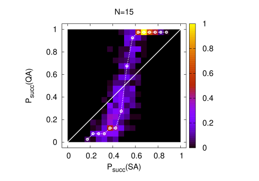
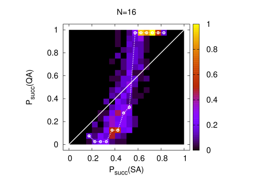
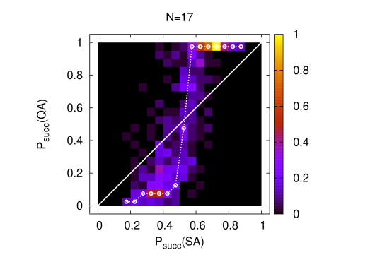
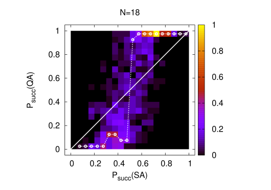
Finally a comprehensive pictorial representation of different quantum versus classical search complexities is obtained in terms of correlations in-between success probabilities $P_{\rm Success}$ for QA and $P_{\rm Success}^{\rm SA}$ for SA, which both are compactified observables on the interval $0\leq P\leq 1$. It is straightforward to construct a double histogram $H(P_{\rm Success}^{\rm SA},P_{\rm Success})$ on the problem set, which counts entry’s into bins and is normalized to unity at the bin of maximal frequency. The data are displayed in Fig. 7) for the largest spin numbers. There is a band of events which parts form the linear correlation, see the straight lines in Fig. 7), and clearly forms a step-like structure at an value of $P_{\rm Success}^{\rm SA}\approx 0.5$. It is clear, and with reference to the arguments of the last section, that we can attribute this step to the presence of catastrophic statistics in the distribution of the quantifier $\Xi_{\rm LZ}$ in eq.(4.6). This issue and the probability distributions of $\Xi_{\rm LZ}$, $\Xi_{\rm GAP}$ and of $P_{\rm Success}$ observables will be discussed in the next section. The work [20] presents similar success rate correlations in-between Dwave and SA again. The step there, see Fig. 2c) of the paper, turns out to be less symmetric with a larger amount of statistical noise. However, the theories definitely are different and nothing quantitative can be concluded from the comparison.

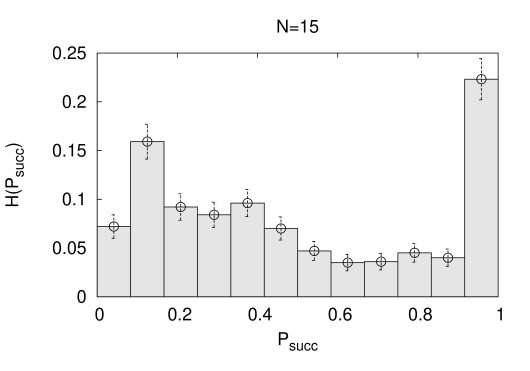
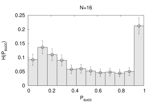
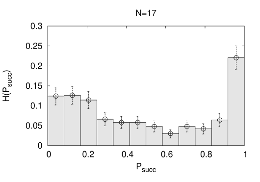
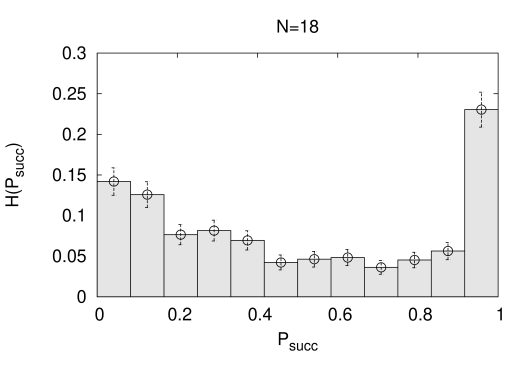
The discretized numerical success probability distribution functions $PDF(P_{\rm Success})$ of the quantum annealing processes on the problem set are bimodal, they span the whole compact interval $[0\leq P\leq 1]$ without any tendency of self-averaging at increasing $N$, and are displayed in Fig. 8) for $N=15,16,17$ and $N=18$. These distributions constitute theoretical predictions for quantum annealer’s that run the linear schedule in the large annealing time ${\cal T}$ limit. The success probability distributions of simulated annealing (SA) are unimodal, as in the case of Dwave [20, 21].

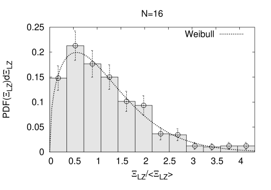
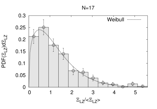
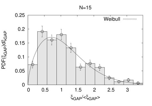
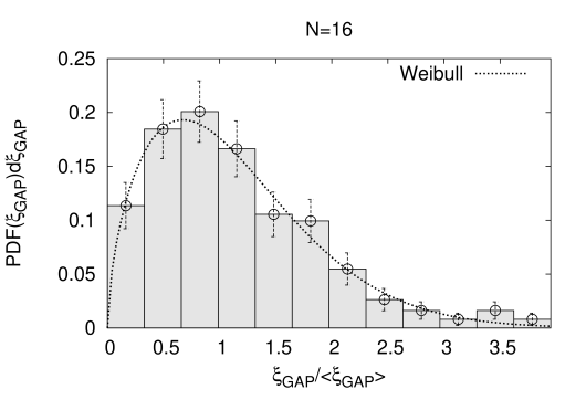
For the linear time schedule the static distributions of $\Xi_{\rm LZ}=\sqrt{\tau_{\rm QA}}$ are relevant, while the $\xi_{\rm GAP}$ gap correlation length distributions at the quantum phase transition anyhow are fundamental. Both kind of probability distributions are displayed Fig. 9): the top row contains $PDF(\Xi_{\rm LZ})$ at $N=16$ and $N=17$, while the bottom row contains $PDF(\xi_{\rm GAP})$ at $N=15$ and $N=16$. On the main diagonal of the figure at $N=16$ one can compare $\Xi_{\rm LZ}$ and $\xi_{\rm GAP}$ PDF’s for an identical problem set. All distributions are plotted as a function of their corresponding variable in units of the median as denoted by $<>$. One notices that the distributions of $PDF(\Xi_{\rm LZ})$ and $PDF(\xi_{\rm GAP})$ at $N=16$ do not differ much, when plotted as a function of median normalized x-coordinates. We have performed fits to the distribution data employing the catastrophic functions $W_{k}$ and $F_{k}$ of eq.(2.16) and eq.(2.17). The qualities of the fits single out Weibull functions $W_{k}$ as the better models for data and, thus we fit e.g. the Ansatz

to the $\xi_{\rm GAP}$ distribution. The fit-results for parameters $k[\xi_{\rm GAP}]$, scales $\xi_{0}$ and correspondingly $k[\Xi_{\rm LZ}]$ and scales $\Xi_{0}$ are all collected in Table 2), together with the $\chi^{2}_{d.o.f}$ values for the fits. The fitted curves are also displayed in Fig. 9), see the curves in the figure. Most importantly we find that for our largest systems at $N=14,...,18$ Weibull functions describe the PDF’s to good precision, see the $\chi^{2}_{d.o.f}$ values in Table 2). This implies thin catastrophic distribution function tails in the variables $\Xi_{\rm LZ}$ or $\xi_{\rm GAP}$. The value of $k$ slowly decreases from $k=1.65$ respectively $k=1.40$ at $N=15$, to $k=1.24$ respectively $k=1.15$ at $N=18$ and possible assumes $k=1$ at infinite $N$. None of the distributions has reached its stationary shape. We mention that a duality in-between $W_{k}$ and $F_{k}$ implies, that Weibull distributions for gap correlation length values turn into Frechet distributed energy gap distributions at $k$. Neither the semi Poisson distribution of nearest neighbor levels in randomly distributed energies $P(\Delta E)d\Delta E\propto\Delta E{\rm exp}[-\Delta E/\Delta E_{0}]$ , nor Wigner’s surmise [43] $P(\Delta E)d\Delta E\propto\Delta E{\rm exp}[-(\Delta E/\Delta E_{0})^{2}]$ of energy gaps aka random matrix theory for quantum level repulsion in the bulk are appropriate models here. If $k$ actually takes the asymptotic value $k=1$, then $P(\Delta E)d\Delta E\propto(\Delta E)^{-2}{\rm exp}[-\Delta E_{0}/\Delta E]$ is predicted with a fat tail in $\Delta E$ ! Znidaric in [44] found a Poisson distribution for the energy gaps in 3SAT with a thin tail in $\Delta E$ however.

There is a simple question: does quantum annealing with the help of quantum fluctuations perform differently, than classical annealing under the use of thermal fluctuations for a given problem set ? Or on the practical side: Can quantum annealing outperform classical annealing ? The issue here is narrowed down to the very specific comparison of the findings in LZ theory (QA) to the numerical data of simulated annealing (SA). The scope of the comparison is limited and can possibly be broadened in sub-sequent work. On the quantum side neither finite run-time corrections to LZ-theory via the excitations to higher energy levels, nor the corrections due to non-linear schedules are accounted. On the classical side physical dynamics is approximated by Monte Carlo pseudo dynamics which one may conjecture to perform faster than genuine classical dynamics. We think that neither restriction is relevant here as efficiencies turn out to be grossly different and likely can not be leveled by corrections.

We display in Fig. 10) our findings with respect to classical dynamics. The logarithmic search time ${\rm ln}\tau_{\rm SA}$ of eq.(3.3) in units of Monte Carlo steps is displayed as a function of the spin number $N$ for a selected sub-set of Deciles on the problem set. For spin numbers $N\geq 10$ up to $N=18$ we find a exponential run time singularity of the form

and the fitted rate constants $r_{\rm SA}$ for various Deciles $D1,D3,D5,D7$ and $D9$ are presented in Table 3). Statistical error bars have been determined with jack-knife binning methods. The numerical rate constant value in the median (D5) is $r_{\rm SA}=0.330(5)$ and turns out to be identical with the $r_{\rm DOS}=0.329(2)$ value of the corresponding singularity in the density of states $\Omega_{1}(N)$. There is a certain spread in the rate constant values pending on the Decile value, which however is bounded and thus our problem ensemble is pure: There is no indication for an admixture of problems, that for small Deciles would either show polynomial, or otherwise different from exponential run time behavior at large Deciles. A similar conclusion can be obtained for the quantum case.

We display in Figures 11 a) and 11 b) our findings with respect to quantum search complexity. The logarithmic gap correlation length ${\rm ln}\xi_{\rm GAP}$ is given in Fig. 11 a) while the logarithmic run time root ${\rm ln}\Xi_{\rm LZ}$ with $\Xi_{\rm LZ}=\sqrt{\tau_{\rm QA}}$ is given in Fig. 11 b). Again we present data for a selected set of Deciles including the median. We observe a crossover behavior from weak singular behavior at small $N$ turning to strong singular behavior at largest $N$. For spin numbers $N\geq 14$ and for both observables the data are consistent with exponential singularities

and

Exponential singular behavior in run-times was also observed by Znidaric in [6] for 3SAT with a strength of the singularity that at given $N$ however was weaker then the one in this paper. The numerical rate constant values in the median (D5) as obtained from fits to the data with $N\geq 14$ are $r_{\rm GAP}=0.553(6)$ and $r_{\rm LZ}=0.592(8)$ and are given in Table 4). The fitted values of rate constants for other Deciles and corresponding fit quality values $\chi^{2}_{d.o.f.}$ can also be found in Table 4). The rate constant $r_{\rm LZ}$ turns out to be ten percent larger than $r_{\rm GAP}$ and all the fits have $\chi^{2}_{d.o.f.}$-values of ${\cal O}(1)$ indicating good quality data modeling.

Summarizing, using a conventional standard quantum adiabatic algorithm with a transverse field and a linear time schedule we find a ground state quantum search complexity for the ensemble of hard 2SAT problems [3] with a super hard

run time singularity at $r_{\rm QA}={1.184(16)}$, that even exceeds the $2^{N}$ singularity of trivial enumerations. The corresponding singularity in classical, i.e. simulated annealing (SA) searches has a rate constant $r_{\rm SA}$ which only is a fraction $r_{\rm SA}/r_{\rm QA}\approx 0.34$. A compute time wall of such magnitude for an adiabatic quantum algorithm designed to solve the 2SAT problem is theoretically interesting, but from an algorithmic point of view can only be termed an failure. Finally, and recalling that our problems are actually in ${\cal P}$, we state the obvious fact that quantum annealing, as well as classical annealing are not able to recognize a mathematical structure which otherwise and using calculus makes the problem solvable in polynomial time. It is unclear as to which basis for the degrees of freedoms, or which Hamiltonian had to be chosen in 2SAT in order that annealing can succeed in polynomial time, or whether that is possible at all.

References

- [1] S. A. Cook, Proc. Third Annual ACM Symposium on the Theory of Computing, (ACM, New York, 1971) 151.
- [2] J. Stat. Phys. , 144, Issue 3, (2011) 519.
- [3] T. Neuhaus, ”Monte Carlo Search for Very Hard KSAT Realizations for Use in Quantum Annealing”, preprint, November 2014.
- [4] B. Bollobas, C. Borgs, J. T. Chayes, J. H. Kim and D. B. Wilson, ”The scaling window of the 2-SAT transition”, Random Structures and Algorithms 18, Issue 3, (2001) 201.
- [5] M. Znidaric, "Single-solution Random 3-SAT Instances", arXiv:cs/0504101 (2005) preprint.
- [6] M. Znidaric, Phys. Rev. A 71 (2005) 062305.
- [7] S. Kirkpatrick, C. D. Gelatt and M. P. Vecchi, Science, New Series, Vol. 220, No. 4598, 671 (1983).
- [8] A. Apolloni, C. Carvalho and D. de Falco, Stoc. Proc. Appl. 33,(1989) 233-244.
- [9] P. Amara, D. Hsu and J.E. Straub, J. Phys. Chem. 97 (1993) 6715.
- [10] A.B. Finnila, M.A. Gomez, C. Sebenik, C. Stenson and J.D. Doll, Chem. Phys. Lett. 219 (1994) 343.
- [11] T. Kadowaki and H. Nishimori, Phys. Rev. E 58, (1998) 5355.
- [12] T. Morita and H. Nishimori, J. Math. Phys. 49 (2008) 125210.
- [13] M. Ohzeki and H. Nishimori, ”Quantum annealing: An introduction and new developments”, Journal of Computational and Theoretical Nanoscience 8, Number 6 (2011).
- [14] E. Farhi, J. Goldstone, S. Gutmann, and M. Sipser, arXiv:quant-ph/0001106, (2001); E. Farhi, J. Goldstone, S. Gutmann, J. Lapan, A. Lundgren, and D. Preda, Science 292, (2001) 472.
- [15] G. E. Santoro, R. Martonak, E. Tosatti, and R. Car, Science 295 (2002) 2427.
- [16] R. Martonak, G. E. Santoro, E. Tosatti, Phys. Rev. B 66 (2002) 094203.
- [17] G. E. Santoro and E. Tosatti, J. Phys A 39 (2006) R393.
- [18] A. Das and B. K. Chakrabarti, Rev. Mod. Phys. 80 (2008) 1061.
- [19] B. Altshuler, H. Krovi and J. Roland, ”Anderson localization makes adiabatic quantum optimization fail”, PNAS 107 no. 28 (2010) 12446.
- [20] S. Boixo, T. F. Ronnow, S. V. Isakov, Z. Wang, D. Wecker, D. A. Lidar, J. M. Martinis and M. Troyer, Nature Physics 10 (2014) 218.
- [21] T. F. Ronnow, Z. Wang, J. Job, S. Boixo, S. V. Isakov, D. Wecker, J. M. Martinis, D. A. Lidar and M. Troyer, Science 345 (2014) 420.
- [22] B. Heim, T: F. Ronnow, S: V. Isakov, M. Troyer, “Quantum versus Classical Annealing of Ising Spin Glasses”, arXiv:1411.5693 (2014).
- [23] D. A. Battaglia, G. E. Santoro and E. Tosatti, Phys. Rev. E 71 (2005) 066707.
- [24] A. P. Young, S. Knysh, and V. N. Smelyanskiy, Phys. Rev. Lett. 101, 170503 (2008) and Phys. Rev. Lett. 104, 020502 (2010).
- [25] I. Hen and A. P. Young, Phys. Rev. E 84 (2011) 061152.
- [26] E. Farhi, D. Gosset, I. Hen, A. W. Sandvik, P. Shor, A. P. Young and F. Zamponi Phys. Rev. A 86 (2012) 052334 .
- [27] T. Neuhaus, M. Peschina, K. Michielsen and H. De Raedt, Phys. Rev. A 83 (02011) 012309.
- [28] M. H. Amin, A. Y. Smirnov, N. G. Dickson and M. Drew-Brook "Approximate diagonalization method for large-scale Hamiltonians", Phys. Rev. A 86, (2012) 052314.
- [29] J. Brooke, D. Bitko, T.F. Rosenbaum and G. Aeppli, "Quantum annealing in a disordered magnet", Science 284 (1999) 779.
- [30] T. Neuhaus, "Statistical Analysis for Quantum Adiabatic Computations: Quantum Monte Carlo Annealing", Physics Procedia 15 (2011) 71.
- [31] H. de Raedt, Europhys. Lett. 3 (1987) 139.
- [32] Y. Matsuda, H. Nishimori and H. G. Katzgraber, "Ground-state statistics from annealing algorithms: Quantum vs classical approaches", New J. Phys. 11 (2009) 073021.
- [33] B. A. Berg and T. Neuhaus, Phys. Rev. Lett. 68, 9 (1992).
- [34] L. Landau, Physikalische Zeitschrift der Sowjetunion 2, (1932) 46.
- [35] C. Zener, Proceedings of the Royal Society of London A 137 (1932) 696.
- [36] O. Melchert and A.K. Hartmann, ”Ground states of 2d +-J Ising spin glasses via stationary Fokker-Planck sampling”, J. Stat. Mech. P10019 (2008).
- [37] S. Wansleben, J. G. Zabolitzky and C. Kalle, J. of Statist. Phys. 37, Issue 3-4 (1984) 271.
- [38] G. Bhanot, D. Duke and R. Salvador, J. Stat. Phys. 44, Issue 5-6 1986) 985.
- [39] G. Marsaglia, J. Stat. Software 8, 14, (2003) 1.
- [40] D. Browne, ”Quantum computation: Model versus machine”, Nature Physics 10 (2014) 179.
- [41] J. A. Smolin and G. Smith, ”Classical signature of quantum annealing”, preprint arXiv:1305.4904 [quant-ph] (2013).
- [42] S. W. Shin, G. Smith, J. A. Smolin and U. Vazirani, ”How Quantum is the D-Wave Machine?”, preprint arXiv:1401.7087 [quant-ph] (2014).
- [43] E. P. Wigner, in Conference on Neutron Physics by Time-of-Flight (Oak Ridge National Laboratory Report No. 2309, 1957) p. 59.
- [44] M. Znidaric, Phys. Rev. A 72 (2005) 052336.
- [45] H. G. Katzgraber, F. Hamze and R. S. Andrist, "Glassy Chimeras could be blind to quantum speedup: Designing better benchmarks for quantum annealing machines", Phys. Rev. X 4 (2014) 021008.
- [46] W. Vinci, T. Albash, A. Mishra, P. A. Warburton and D. A. Lidar in "Distinguishing Classical and Quantum Models for the D-Wave Device", arXiv:1403.4228 [quant-ph] (Submitted on 17 Mar 2014).
- [47] V. Choi in "Adiabatic Quantum Algorithms for the NP-Complete Maximum-Weight Independent Set, Exact Cover and 3SAT Problems", preprint arXiv:1004.2226 [quant-ph] (Submitted on 13 Apr 2010).