Quantum simulation of -dimensional U(1) gauge-Higgs model on a lattice
by cold Bose gases
Abstract
We present a theoretical study of quantum simulations of -dimensional U(1) lattice gauge-Higgs models, which contain a compact U(1) gauge field and a Higgs matter field, by using ultra-cold bosonic gases on a one-dimensional optical lattice. Starting from the extended Bose-Hubbard model with on-site and nearest-neighbor interactions, we derive the U(1) lattice gauge-Higgs model as a low-energy effective theory. The derived gauge-Higgs model exhibits nontrivial phase transitions between confinement and Higgs phases, and we discuss the relation with the phase transition in the extended Bose-Hubbard model. Finally, we study real-time dynamics of an electric flux by the Gross-Pitaevskii equations and the truncated Wigner approximation. The dynamics is governed by a bosonic analog of the Schwinger mechanism, i.e., shielding of an electric flux by a condensation of Higgs fields, which occurs differently in the Higgs and the confinement phase. These results, together with the obtained phase diagrams, shall guide experimentalists in designing quantum simulations of the gauge-Higgs models by cold gases.
pacs:
11.15.Ha, 67.85.HjI Introduction
To understand physics of a given quantum many-body system in a coherent manner is not an easy matter. For example, the time development of these systems have not been clarified enough because high dimensionality of the state-vector space brings great difficulty for solving many-body Schrödinger equation Noack . The sign problem also prevents us from carrying out straightforward Monte Carlo simulations for models including fermionic matter fields Troyer .
In the last several years, as an alternative approach, quantum simulations of various quantum systems by using ultra-cold atomic gases on an optical lattice have attracted lots of interests coldatoms . This comes mainly from high controllability and versatility of such atomic systems. Quantum simulations of systems under a synthetic gauge field have already become feasible due to experimental developments mg_optical . Furthermore, recent studies have proposed several ideas for realizing simulators of quantum systems involving dynamical gauge fields WieseZohar . Gauge systems appear in various fields of physics as an effective model, and to understand their dynamics is one of the most important problems. Also, proposals for an experimentally feasible atomic simulator of gauge systems still remain as an open problem.
In the previous papers U1GHM ; NJP1 ; Future , some of the present authors discussed how to simulate lattice gauge-Higgs models (GHMs) Fradkin ; ichimaturev by bosonic atoms on a -dimensional optical lattice ( in Refs. U1GHM ; Future and in Ref. NJP1 ). The starting model in that approach is a cold atomic system described by the extended Bose-Hubbard model (EBHM) Baier ; Dutta ; a lattice model of bosons having both on-site and off-site interactions. The target gauge model, GHM, is a U(1) lattice gauge theory wilson involving a compact U(1) gauge field and a Higgs field in the London limit. Reflecting the nonrelativistic nature of the EBHM, interactions in the GHMs are asymmetric in the space and time directions; some couplings in the spatial directions have no partners in the time direction in contrast to the lattice gauge theory considered in high-energy physics wilson . However, the GHMs have a very interesting phase diagram as we shall see, and quantum simulation of the GHMs is expected to give us a very useful insight on the dynamics of the gauge theory.
In this approach U1GHM ; NJP1 ; Future , the phase degree of freedom of boson operator on the site of the optical lattice plays the role of the compact U(1) gauge field defined on the link of a -dimensional (spatial) lattice of lattice gauge theory ( is the direction index). Compared with the alternative approach called quantum link model (gauge magnet) quantumlink , this approach has an advantage to express a compact U(1) gauge theory in terms of the genuine U(1) operator advantage . The Hamiltonian of the EBHM is known to contain an annoying term that breaks Gauss law of the pure gauge theory (i.e., theory containing no matter fields) and forces one to make a severe fine-tuning of its coefficient to generate a local gauge symmetry WieseZohar . However, inclusion of the Higgs field converts this breaking term to a term expressing the genuine Gauss-law with Higgs charge and relieves us from the fine-tuning.
In this paper, we consider theoretically the atomic quantum simulation of the GHM with , supposing a system of Bosonic atoms on a one-dimensional (1D) optical lattice. This work is motivated by the following reasons:
(i) From experimental point of views, quantum simulation of gauge theories in a 1D spatial lattice is expected to be easier than that in higher-dimensional lattices WieseZohar . The present approach is based on a set of single-component atoms with long-range interaction (e.g., dipole-dipole interaction) loaded on a 1D optical lattice. It has the following advantages advantage ; first, this set up is proved to be feasible experimentally 1Doptical_DDI . Second, a digital quantum simulation of the Schwinger model has been realized recently by using a 1D chain of several sites of trapped ions Martinez . In contrast, the present 1D optical lattice is scalable, i.e., hundreds of sites with large number of atoms can be prepared. Third, some approaches such as Ref. Bazavov use the quantum link model, whose realization requires two-component atoms on the optical lattice. The single-component atoms in the present approach is certainly more feasible in experiments.
(ii) We can expect nontrivial behavior of the phase transitions of the target GHM, not found in the higher-dimensional cases U1GHM ; NJP1 ; Future . As shown later, the phase transition is governed by the Berezinskii-Kosterlitz-Thouless (BKT) type transition BKT .
(iii) Non-equilibrium physics of the lattice gauge theories has not been deeply understood yet. This subject is closely related to the recent heavy-ion collision experiments in high-energy physics HIC . In our previous paper NJP1 ; Future , we applied the Gross-Pitaevskii (GP) model GP to study the real time dynamics of an electric flux, showing that the dynamics qualitatively realizes the behavior expected in each phase of the GHM. On the other hand, since the quantum fluctuations become more important in 1D system, we should include some quantum correction to the GP approach. Actually, real-time dynamics of a lattice gauge model has been studied by tensor network method TNN , which is mainly applicable for 1D quantum systems with low filling. Here, we use the truncated Wigner approximation TWA to study the effects of quantum fluctuations.
Let us explain the basic steps of the present paper. First, by applying the method in our previous papers U1GHM ; NJP1 ; Future to the 1D EBHM for large fillings of atoms (large average occupation numbers of atoms per site) we obtain the (1+1)D GHM with short-range interactions. Here the additional +1D in the GHMs represents the imaginary-time axis in path-integral quantization for which we also use a lattice regularization. Next, we calculate the phase diagram of the derived GHM, which contains the Higgs phase and the confinement phase separated by the BKT transition. This phase diagram is compared with that of the EBHM to discuss the interesting relations between the strongly-correlated bosons and the gauge systems; namely, the Higgs phase corresponds to the superfluid phase and the confinement phase to Mott-insulator phase. This also provides an estimation of the relevant parameter region to simulate the phase transitions in experiments. Finally, we study the real-time dynamics of the GHM by using the GP equation GP and the truncated Wigner approximation TWA . This mean-field approach naturally arises because of the assumption of the large fillings of atoms. Numerical results show that a prepared electric flux exhibits quite different behaviors depending on the Higgs or confinement phase. A phenomenon similar to the Schwinger mechanism is observed numerically.
The paper is organized as follows. In Sec. II, we present a derivation from the experimentally realized model, the EBHM on the 1D optical lattice, to the target simulated model, the (1+1)D U(1) GHMs which follows our previous works U1GHM ; Future . In Sec. III we discuss the phase diagram of the GHM calculated by the Monte Carlo simulations. The obtained phase diagram is compared with that of the EBHM, whose details of the calculation is described in Appendix A. In Sec. IV, we study non-equilibrium physics of the GHM, especially focusing on real-time dynamics of an electric flux. We present conclusion in Sec. V
II Relation between the extended Bose-Hubbard model and the gauge-Higgs model
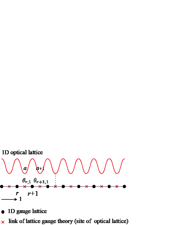
We start with the EBHM defined on a 1D optical lattice (see Fig. 1). The hamiltonian is given as
| (1) |
where and are creation and annihilation operators of bosonic atoms on the site , respectively, satisfying , etc. By representing , we have the phase operator and the density operator . The coefficient represents the hopping strength, the on-site interaction, and the nearest-neighbor (NN) replusive interaction generated by, e.g., a dipole-dipole interaction DDI . The above on-site repulsion represents the sum of -wave scattering interaction and on-site dipole-dipole interaction ; . The -wave scattering amplitude is highly controllable by Feshbach resonance Feshbach and the hopping is controlled by the strength of the laser that makes the optical lattice. On the other hand, the NN repulsion is determined by the kind of the atoms loaded on the lattice and also depends on the lattice spacing. In particular, ratios and can become highly-controllable parameters in real experiments by changing lattice depth coldatoms and -wave scattering lengths Feshbach , respectively.
The procedure U1GHM ; NJP1 ; Future to derive the GHM with local interactions from the EBHM for homogeneous density average at large fillings is based on a couple of assumption; (i) the average density is homogeneous and large, (large filling) and (ii) the density fluctuation around is small. The point (ii) implies that we focus on the sector of low-energy excitations. Explicitly, we write the density operator as
| (2) |
and expand with respect to the fluctuation operator up to the second-order. This kind of expansion is widely used in atomic physics coldatoms .
To regard this expanded Hamiltonian as that of the GHM, we introduce a gauge lattice and a set of operators in gauge theory defined on it. The gauge lattice is the dual lattice of the optical lattice (see Fig. 1); the site of the gauge lattice sits on the middle point of the link of the optical lattice. We define the 1st component of the vector potential and its conjugate momentum, namely the electric field , on the gauge link as
| (3) |
where we use the same character both for atomic and gauge variables (They can be distinguished by whether it carries the direction suffix 1). Strictly speaking, the electric field should carry the direction suffix 1 as , but we omit it in this paper because there are no other components in a 1D system. On the other hand, we keep the suffix 1 in because we shall introduce the zeroth component of vector potential later [see in Eq. (10)]. These pairs satisfy the canonical commutation relations wilson ,
| (4) |
which come from the commutation relations of . The factor in Eq. (3) may look curious but is necessary to generate the Gauss law as we shall see. Then the expanded Hamiltonian up to is expressed as
| (5) |
where we omitted hat symbols for operators. There appear no terms linear in because is chosen such that it gives rise to a stationary point of the energy. is an irrelevant constant. The hopping term of Eq. (1) generates both the last term of and the term . Their coefficients are and respectively, and the latter is suppressed by an extra factor for large fillings. Therefore we neglect and keep as the Hamiltonian of the GHM for large fillings.
The first term of leads to Gaussian with respect to , the divergence of the electric field, and gives rise to . This becomes the Gauss-law constraint for pure gauge theory in the limit , and this limit is just the fine tuning required for the pure gauge theory in Refs. WieseZohar . After introduction of a Higgs field in the London limit, this term represents the genuine Gauss law () with the Higgs charge (see Ref. Future for details).
The second term represents the energy of electric field. In the ordinary lattice gauge theory used in high-energy physics wilson , its coefficient is the square of so called real gauge coupling constant and is treated as positive definite. In our case, may take negative value (although we used a suggestive notation that it may be positive). Here we can see that a homogeneous configuration of is realized for by using a very simple type of the mean-field theory, i.e., two site mean-field theory. We take only two nearest-neighbor site of the Hamiltonian , called even-site and odd-site. By putting a mean field ansatz and into the two sites, the EBHM mean field energy , which depends on the two mean density is given as
| . | (6) |
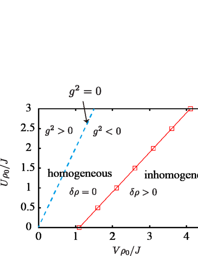
Then by detecting the energy minimum under a canonical ensemble constraint, , we can show the homogeneity of the atom density. Fig. 2 indicates the homogeneity of the atom density in (-)-plane. Here, we found that, is homogeneous for , i.e., , while for , takes an inhomogeneous DW configuration such as (see Fig. 2). Result in Fig. 2 also indicates the existence of a homogeneous ‘phase’ even for . This comes from the fact that the ‘critical line’ is renormalized by the hopping -term in in Eq. (1). In Appendix A, we give rather detailed discussion on this homogeneous state and obtain the global phase diagram of the EBHM.
The third term of expresses the NN coupling of the U(1) gauge field as + H.c., but it breaks the gauge symmetry under ( is an arbitrary -dependent real parameter) wilson . In Refs. U1GHM ; NJP1 ; Future we introduced a U(1) Higgs field in the London limit (its amplitude is frozen to unity) on the site , and regard this term as a gauge-fixed version of the Higgs coupling to the unitary gauge as
| (7) | |||||
This Higgs coupling and the remaining terms in is invariant under the local U(1) gauge transformation wilson
| (8) |
where the bar symbol in denotes the complex conjugate. In short, is a gauge-invariant Hamiltonian which we formally work with and the gauge invariant observables are calculable by its gauge fixed version of Eq. (5).
Here we comment that, in the present 1D system, the Gauss law term of gauge theory is to be supplied only by the - and -terms in . This is in contrast with the higher dimensional [(2+1)D and (3+1)D] systems in which one must take additional next-NN interactions into account NJP1 ; Future . This point shows that the 1D atomic system is more feasible to realize a quantum simulator in experiments than the higher dimensional systems.
To derive the gauge model, we start with the partition function defined from of Eq. (5) with the inverse temperature expressed in path-integral in canonical formalism (sum over canonical pair of coordinate and momentum). Then all the fields are defined on the (1+1)D lattice with its site denoted by as , where is the site index along the imaginary-time axis discretized by the spacing and we take the limit formally. In this paper we omit the hat symbol in to denote the unit vector in the -th direction. Therefore and imply the NN site and respectively. We use as the forward difference operator .
We introduce the imaginary-time () component of the gauge field on the link to make the first Gauss-law term of a linear form in , i.e.,
| (9) |
Because every step in the approach of Refs. U1GHM ; NJP1 ; Future is applied in the present (1+1)D system in a straightforward manner, we present the expressions for as (For details see Sec. II of Ref. Future ),
| (10) |
The action may be expressed in terms of the compact U(1) variables on the link and as
| (11) |
The parameters in are expressed in terms of those in and as
| (12) |
The action in Eq. (11) contains only the short-range interaction, and each term is obviously invariant under a time-dependent local gauge transformation [given by Eq. (8) with the replacement ], and the term is nothing but the gauge-invariant kinetic term of the Higgs field Fradkin . The present action (11) is derived from the nonrelativistic Hamiltonian (1) and has no relativistic invariance under change of directions , which is in contrast with the conventional models wilson in lattice gauge theory. However, this model supports both the confinement and Higgs phases (see Sec. III) and therefore is interesting enough for simulation of the gauge theory.
III Phase diagram of the GHM
In this section we calculate the phase diagram of the GHM defined by Eqs.(10) and (11) by MC simulations. For ordinary second-order phase transitions, one may use the specific heat ,
| (13) |
to locate the transition point by the peak of . However, because the present GHM is a (1+1)D system with a global U(1) symmetry as we shall see, the general theorem allows neither second-order transition nor long-range order. One may expect, if any, a phase transition of the same type as the BKT transition that is well known in the 2D XY spin model BKT . This expectation is plausible because the original 1D EBHM itself is known to have a phase transition at zero temperature between the Mott-insulator and superfluid, where the superfluid has a quasi-long range order due to the low dimensionality of the space.
Let us summarize the 2D XY spin model and its BKT transition. Its action is given by
where is the XY spin angle defined on and . The BKT transition of the 2D XY model is of infinite order, signaled by divergence of the susceptibility ,
| (15) |
at the transition point . This value deviates from the round peak of specific heat by . The spin-spin correlation function for large behaves exponentially in the spin disordered () phase and algebraically in the spin quasi-ordered () phase. The correlation length and the critical exponent depend on as near and .
To locate the phase transition point, one may observe the scaling behavior of of Eq. (15) for lattice of size with the periodic boundary condition. In the quasi-ordered phase, power decay of gives rise to for large . One may define the scaled susceptibility density as with arbitrary parameter . Then one has
| (16) |
Therefore, at , becomes scale invariant (no -dependence). We note that this scale invariance holds for every point of . Among possible multiple set of scale-invariant points , the smallest value of is just the critical point . On the other hand, in the disordered phase, behavior of depends on the relation between and . For (i.e., is well below ), the exponential decay of gives rise to and , which shows no scale-invariant points are possible (for ). For other case (), no explicit formula of seems available. Although there is no analytic proof that has no scale invariant points throughout the disordered phase, we confirmed that it is the case by numerical analysis applying the same method to obtain Fig. 3(d).
Below we shall see a close relation between the GHM and the 2D XY model, and explore the possibility of a BKT-type phase transition of the GHM. Let us first consider the limit of . Then of Eq. (11) forces (mod )] up to gauge rotation. By introducing the gauge-invariant angle variable (we use the same letter as the above XY spin angle) on the spatial link [i.e., between the site and ] as
| (17) |
reduces up to a constant to
| (18) |
This is just the action of the 2D XY spin model with the asymmetric couplings and . It has the global U(1) symmetry under . This limiting model exhibits BKT transitions on a certain critical line in the - plane asymXY .
As is reduced from infinity, is allowed to fluctuate more.
However, it is plausible to expect that the above critical line in the -
plane survive for finite but large enough , and the BKT-type scaling relation
(16) holds. Then, we determine the transition point for a given set of
using the scaled susceptibility density of Eq. (16)
calculated by and Eq. (17).
Explicit procedures are as follows;
(i) Fix and and measure the susceptibility along for
three ’s ().
(ii) Obtain interpolating curves
for in third-order polynomials in ;
(iii) For (below we use instead of
because no confusions may arise) , set the conditions
of a triple intersection;
, and solve these two equalities numerically.
From Eq. (16), one expects
a continuous (multiple) set of solutions for every value of
starting at and larger than the critical value .
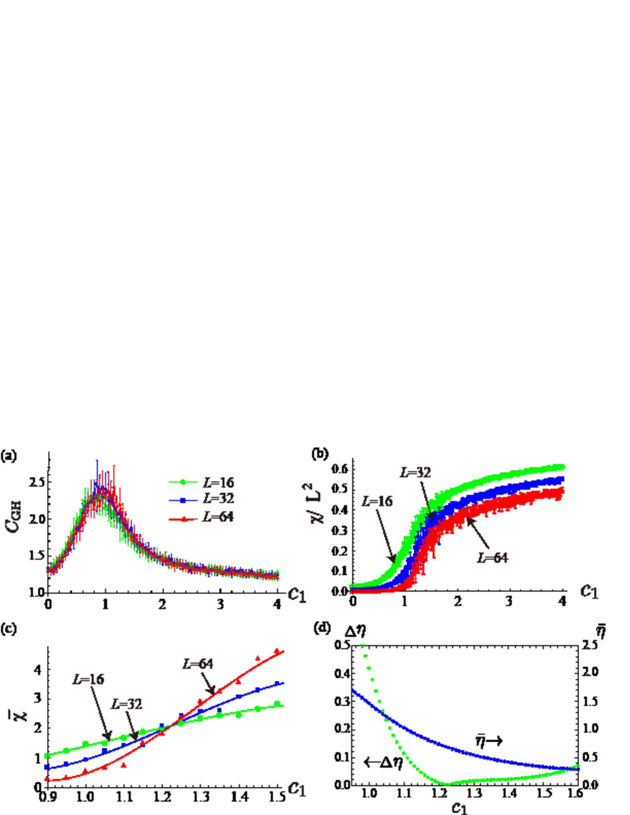
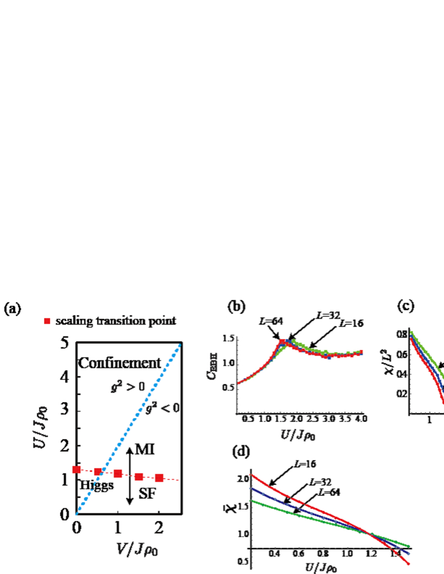
In Fig. 3, we show (a) and (b) susceptibility density for and , , . Instead of multiple set of solutions, we find a unique triple intersection at for . In Fig. 3 (c) we show three with this value. To understand the absence of multiple solutions, we introduce the distance from the triple interaction defined as follows; Each pair of three curves (e.g., and ) with fixed has an intersection at . We define Max of three distances, . In Fig. 3 (d) we show together with the average of , . The triple intersection at locates at the unique minimum of and separates the large -region ( and the small -region (). By regarding in almost vanishing, Eq. (16) tells us that the point is an approximate critical point of BKT-type phase transition separating the disordered phase () and the quasi-ordered phase ). Slow but steady development of from zero with increasing shows that there exist some corrections to the power-law decay of spin correlations. One may account for it by finite-size effect generally; in particular, by the logarithmic corrections janke that may become relatively important for smaller . Then, we expect that for tends to small if we use the date obtained for systems with larger . To calculate the critical point for general below, we repeat to identify a unique triple intersection (scale-invariant point) as the BKT-type critical point. This manipulation is supported because a quite similar behavior of is observed for the 2D XY model giving rise to in good agreement with the known results in parentheses for larger .
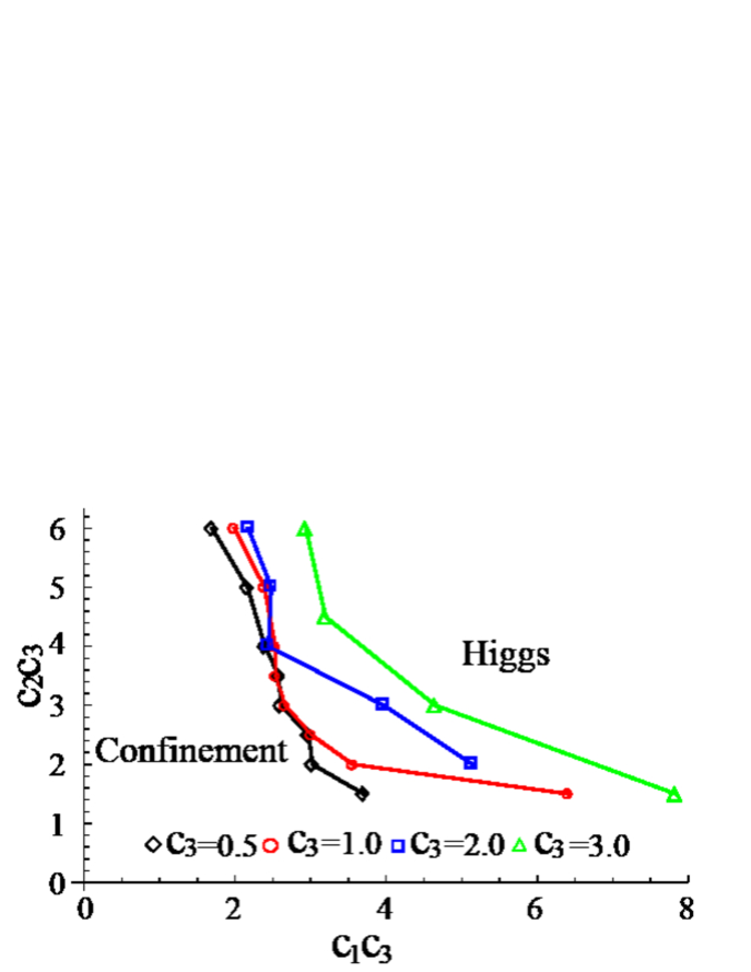
In Fig. 4, we show the phase diagram in the (-) plane obtained in the same procedure as in Fig. 3 (c). The four transition lines correspond to and . The two coordinates and of this plane are chosen so that they are dimensionless and independent combinations (see Sec. III of Ref. Future for detailed discussion on this point). We note that there are no transitions in the region of because the data fitting in the form of Eq. (16) failed there. This is consistent with our assumption that finite but sufficiently large is a necessary condition for BKT-type transition.
Because the disordered phase necessarily realizes for small ’s, the lower (smaller ) region in Fig. 4 corresponds to the disordered phase, and the higher (larger ) region corresponds to the quasi-ordered phase. In gauge theory, typical and well-known phases are Higgs, confinement, and Coulomb phases. The magnitude of fluctuations of gauge field increases in this order wilson ; Kogut ; Fradkin . The magnitude of fluctuations of conjugate electric field decreases in this order due to the uncertainty principle. Because we have two phases in Fig. 4, we naturally identify the spin-disorder phase as the confinement phase and the quasi-ordered phase as the Higgs phase. This is supported by the phase diagrams obtained for related GHMs derived from the 2D and 3D EBHM U1GHM ; NJP1 ; Future .
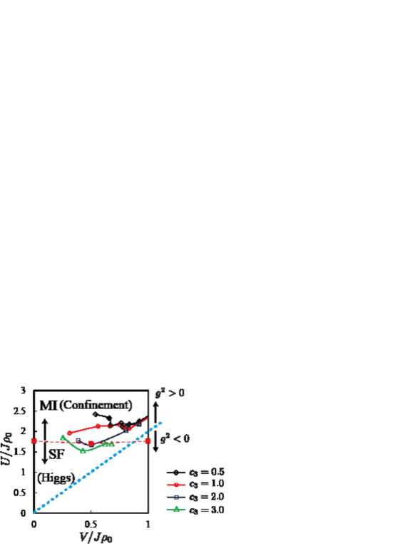
In order to identify the relevant parameter regions in experiments, it is important to compare the phase diagram of Fig. 4 to that of the original EBHM Eq. (1). In Fig. 5, we show the phase diagram of the EBHM in small regime, which is obtained by the MC simulations in Appendix A. There are two phases. In the Mott insulator (MI) phase, the strong on-site repulsion stabilizes the uniform distribution of atoms without the phase coherence. For the large hopping , the superfluid (SF) forms as a result of the Bose-Einstein condensation. In Fig. 5, the red dotted line shows the phase boundary of the EBHM between the MI and the SF, which was determined by a scaling method. For details, see Appendix A and Fig. A.1. To compare the phase diagrams of BHM and GHMs, we transport critical lines shown in Fig. 4 to those in the (-) plane of Fig. 5, by using the relations between the parameters such as and . The phase boundaries of the two models are fairly in good agreement for and this result certifies the existence the confinement-Higgs phase transition.
In other words, our target phases are the MI phase and the SF phase in relatively small regime; the two phases in cold atomic system has explicit meaning of the lattice gauge theory. Fig. 5 also shows suitable parameter regions for the quantum-simulation experiment on the GHM. This fact certainly supports that the confinement-Higgs phase transition can be observed by experiments of ultra-cold atoms in a 1D optical lattice.
The phase diagram of the BHM in large regime itself has various interesting phases DMRG1 ; Kawaki . As the NN repulsion is getting larger compared to the on-site repulsion, the assumption of uniform density configuration is broken, and the density wave phase appears in the phase diagram, in which an imbalance in the density at the even and odd sites exists. The result of the MC simulation for large is also given in Appendix A.
IV Real-time dynamics of electric flux string
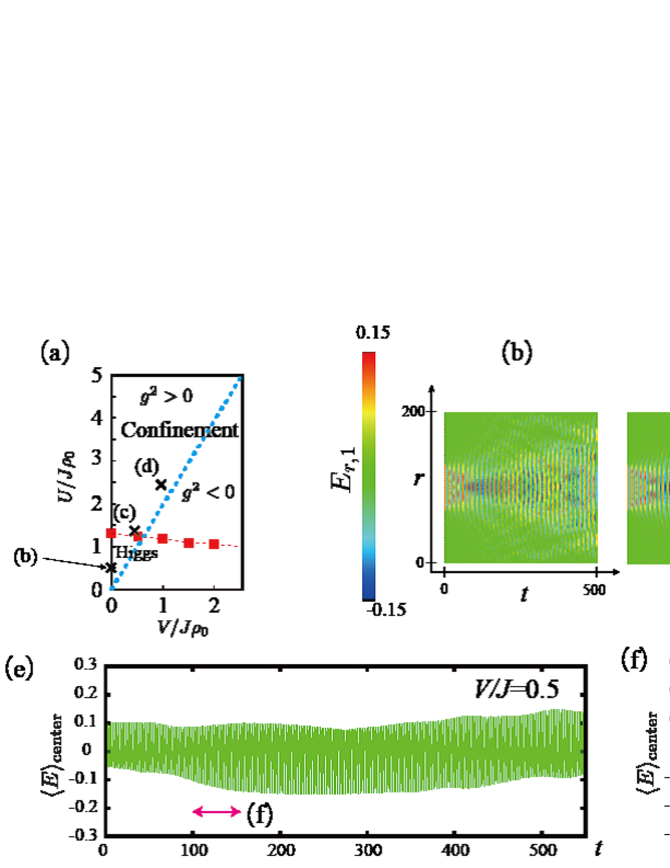
In the high-energy physics, study of non-equilibrium dynamics of the gauge theories in Minkowski space-time has been a challenging problem. Its detailed study is going to be even more important inspired by recent heavy-ion collision experiments HIC . In this section, we study real-time dynamics of an electric flux in the Higgs and confinement phases observed by the path-integral MC simulations in Sec. III. To this end, we employ the GP equation, which is a reliable method to simulate dynamical behavior of a condensed fluid in condensed matter physics especially for the superfluid behavior GP2 . In general the GP equation is suitable for the SF (Higgs) phase, however in this section we extend the limitation, i.e., apply the GP equation to the MI (confinement) phase and focus on investigating qualitative behavior of both phases. A similar problem of real-time dynamics of an electric flux was addressed in an atomic quantum simulation of the Schwinger model, the (1+1)D quantum electrodynamics (QED), in Refs. Schw ; TNN , where the tensor network simulation was used. Interestingly enough, the calculations in Refs. Schw ; TNN report qualitatively different behavior of the electric flux depending on values of the gauge coupling and mass of the electron.
From Sec. III, the present D GHMs have two different phases, the Higgs and the confinement phases, therefore study of dynamical behavior of the electric flux gives important and interesting insight into the gauge dynamics in each phase. A similar problem for the higher-dimensional cases has been already addressed in our previous work NJP1 ; Future , where we have obtained qualitative difference of flux string behavior for each phases. In the present D case, the direct comparison between the GHM in Eq. (5) and the Schwinger model is possible for the string dynamics.
The GP equation can be derived from the coherent path-integral of the EBHM as a saddle point equation. When the Lagrangian is described as , the Euler-Lagrangian equation becomes the GP equation. From this procedure, the GP equation for the EBHM is given by
| (19) | |||||
where we have added chemical potential term by which the average density is controlled. In what follows, we set the equilibrium density by putting . Here it should be remarked that this is a kind of the normalization and results for other densities can be obtained by a simple rescaling as with . A system of spatial lattice sites with the free boundary condition is used and the time step for the numerical calculation is set as . The time scale is 0.32 [msec] by using the energy scale 500[Hz] in typical experiments. In Eq. (19), the dissipation term is not included, and therefore the total energy is conserved during the time evolution.
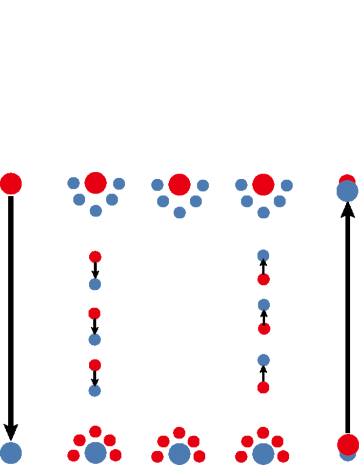
As an example of a non-equilibrium state of the system, we consider the state with a single electric flux with a length , i.e., we set the electric flux string in the initial state and solve the GP equation numerically. Hereafter we use the gauge lattice label, . Explicitly, we set the initial configuration as for ( is the center of the string). On the other sites, . In experiments the above initial flux is created by the density modulation Wurtz . In our numerical simulation, we set the length of the electric flux . In the confinement phase, this length is expected to be long enough for observing the typical quark-confinement phenomena Kogut ; Smit .
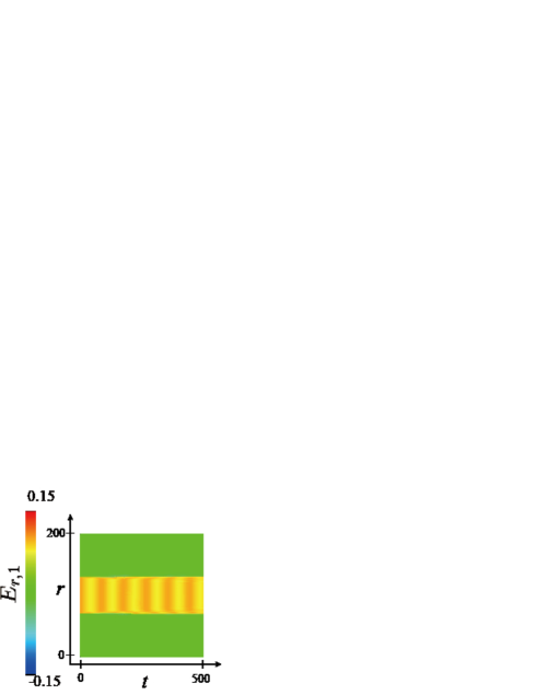
We first briefly consider the case of sufficiently small , and verify that the electric flux string is stable by solving the GP equation (19). In our numerical simulation, the electric field are defined as
| (20) |
This corresponds to a density fluctuation from mean density. The typical numerical results is shown in Fig. 6. When is very small, the effects of the Higgs field is very small and the system has properties of the pure compact U(1) gauge theory.
In Fig. 7 (b)-(d), we show the time development of an electric flux along line in the phase diagram. The results show that from the Higgs phase to the confinement phase, the stability of the electric flux is increased. In fact, there is a striking difference between the Higgs phase and the confinement phase; in the Higgs phase the electric flux spreads out. On the other hand in the confinement phase, the form of the initial flux does not change. In addition, we find that in both phases an oscillation of the electric field in the flux takes place. This behavior of the flux string means that a pair production of the Higgs particle and the resultant string breaking takes place. But in the confinement phase the restoration of the flux string readily occurs as a result of the strong gauge coupling. By contrast, in the Higgs phase the initial electric flux is unstable, i.e., bits of electric flux appear and they spread out from the initial region . This behavior comes from the condensation of the Higgs field and the resultant spontaneous symmetry breaking of the global U(1) gauge symmetry, i.e., the charge is not conserved in the Higgs phase.
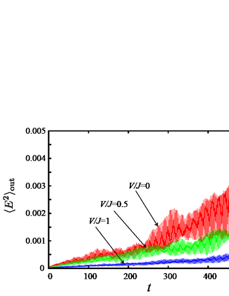
In order to evaluate the spread of the electric field from the initial string, we measure the mean value of electric field strength outside of the initial place of the electric flux,
| (21) |
Fig. 8 shows the for some typical values of the Gauss-law coupling along the line . It is obvious that as the value of decreases, increases rapidly as a function of time, i.e., the initial configuration of the electric flux is unstable, and electric-field excitations propagate out of the initial electric flux.
In addition, Fig. 7 exhibits another remarkable behavior of the electric field as non-equilibrium phenomena. The results show that on the sites, where the initial electric flux exists, the electric fields are oscillating and changing their sign in both the Higgs and the confinement phases. The data in Fig. 7 (e) and (f) shows the time evolution of the electric field averaged over the central ten sites . Similar behavior was observed in all three cases; the central electric field in all cases oscillates in time and takes even negative values. The result is similar to behavior of an electric flux in Schwinger model with a small electron mass as reported in Refs. Schw ; TNN , and the phenomenon is called the string-antistring oscillation. Quantum link version of QED was also studied from this point of view Banerjee . All the above studies indicate that the pair creation takes place in the central region of the electric flux as the Schwinger mechanism tells Schwinger . The two initial static charges residing on the edges of the initial electric flux tend to be shielded by particles of opposite charge. The initial electric flux vanishes as a result. After that, the reverse process happens, i.e., the pair creation recurs and the electric flux in the opposite direction is created. Iterating this process causes consequently the string-antistring oscillation. Our results in Figs.7 (b)-(f) for the U(1) GHM suggest that a similar string-antistring oscillation process takes place as in QED. Fig. 9 illustrates schematically the string-antistring oscillation process.
In the above, we studied the real-time dynamics of the electric flux string by using the GP equation. Results concerning to the Higgs phase are reliable as the Higgs phase is nothing but the SF and the order parameter has only small fluctuations there. On the other hand, one may think that use of the GP equation for the MI regime is not appropriate even in the region close to the phase boundary to the SF. However, we expect that our study for the weak MI regime captures at least qualitatively correct picture of the string dynamics. In fact, the numerical results presented above are very similar to those obtained by other numerical results for closely related gauge models in Refs. Schw ; TNN .
Anyway, a more detailed study of the dynamics of the flux string in the confinement-MI regime is important and it gives some useful remarks on the experimental setup. To this end, the idea of the truncated Wigner approximation (TWA) is useful TWA , that is, we simulate the real-time dynamics of the flux string with different initial conditions. In the above, on solving the GP equation, we employed the initial condition such that the phase of the wave function . However in the MI state, the phase of the ‘condensate’ fluctuates as a result of the uncertainty relation between the particle number and the phase. In other words, the fluctuations of the phase cannot be avoided in the MI even if a prominent experimental technique to control the phase of the ‘condensate’ is used. This fact arises questions about the reliability of the results obtained by the GP equation.
Here, to study the effect of the phase fluctuation, we employ the initial condition such that and solve the GP equation, where the variables are homogeneously distributed random numbers between with . To calculate the physical quantities like the density at each site, we take 100 samples, which have different initial conditions produced by the random numbers , and take average of the calculated quantities over the samples. In this way, we obtain results of the real-time dynamics of the electric flux. This sampling method essentially corresponds to the TWA TWA .
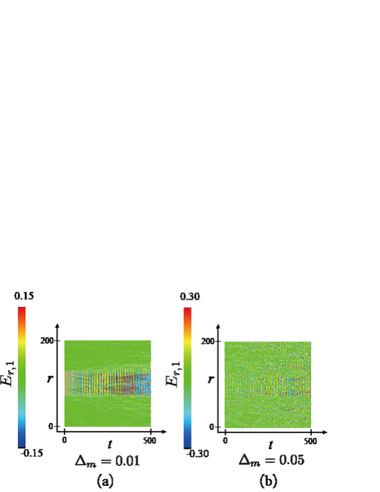
Fig. 10 shows the real-time dynamics of the flux string for the parameters , , which locates in the weak MI region in the phase diagram, and for two cases of the random distribution of the phase, and . The other conditions are the same with those in the previous calculation. For , the stable evolution of the string is observed, whereas for , only small portion of the initial string configuration remains. From the above result and the uncertainty relation of the number and phase, , the fluctuation of the atomic number at the initial state is required as . To satisfy this requirement in experiments, the average particle number must be sufficiently large and also a sufficient number modulation in the flux string is needed. If this condition is satisfied, the string-antistring oscillation in Fig. 7 is to be observed. More detailed study on this problem by using the full TWA and its extension TWA will be reported in a future publication.
Finally let us comment on the real-time dynamics of the flux string in the confinement-MI region apart from the phase boundary to the SF. In this region, the GP equation is not applicable, as the phase of the ‘condensate’ fluctuates rather strongly. However, this region corresponds to the strong-coupling region of the GHM, and therefore the string tension of the electric flux is strong. Then it is naturally expected that the string is quite stable and its fluctuations in time are small, and as a result its electric field is kept positive, . In fact, this phenomenon was observed in the numerical study of the gauge models in Refs. Schw ; TNN .
V Conclusion
We explained how to realize the atomic quantum simulation of the (1+1)D GHM by using cold atomic gases on the optical lattice. By means of the path-integral MC simulations, we obtained the phase diagrams of the GHM and also the EBHM at large filling and verified that these two phase diagrams are in good agreement with each other for the parameter region of the positive gauge coupling. We examined the phases of the EBHM from the gauge-theoretical point of view and the result is summarized in Table 1.
| EBHM | U(1) GHM | ||
|---|---|---|---|
| MI | Confinement | large | (homogeneous) |
| SF | Higgs | small | (homogeneous) |
By using the GP equations for the EBHM, we investigated dynamical properties of the electric flux put on a line as an initial state. In the confinement region of the GHM, the string breaking and restoration of the electric flux is observed, which has similar properties to the Schwinger mechanism in QED. On the other hand in the Higgs region, the flux spreads out and many bits of electric flux develop. Finally we discussed the reliability of the results obtained by the GP equations by using the idea of the TWA, and gave some remarks for the experimental setup to observe the string-antistring oscillation. We hope that the above phenomena will be observed experimentally in the near future. In particular, dynamical behavior of the transition from the confinement to Higgs phases is quite interesting and expected to be observed by the strong controllability and the versatility of the cold atomic system.
Finally, let us note that our approach identifies the phase and the amplitude of atomic variable as U(1) vector potential and the electric field respectively, and introduce the Higgs field to relax the crucial fine tuning to realize the Gauss’ law. These general and universal procedures make us possible to define corresponding GHMs of wide variety both for high and low fillings and also for homogeneous and inhomogeneous atomic distributions. Although this GHM may contain nonlocal interactions in some cases and look quite different from the conventional lattice gauge theory, it is important that GHM is of course a “gauge theory having gauge symmetry”. It obviously opens the way to study gauge theory in more general view points. Also such gauge-theoretical view points may shed some lights backward on studying the original atomic systems as partly shown in Sec. A.3.
Acknowledgements.
Y. K. acknowledges the support of a Grant-in-Aid for JSPS Fellows (No.JP15J07370). This work was partially supported by Grant-in-Aid for Scientific Research from Japan Society for the Promotion of Science under Grant No.JP26400246, JP26400371 and JP26400412.Appendix A Global phase diagram of extended Bose-Hubbard model in the plane for large fillings
In this Appendix, we study the global phase diagram of the 1D EBHM in the whole (-)-plane at large fillings by taking account of both homogeneous and inhomogeneous local density average . To this end, we first derive an effective model, which is to be used for study of the EBHM in the whole parameter region in the (-)-plane, in particular even for a negative . This model includes the local variational density introduced in Ref. Kuno in addition to the spatial vector potential , and is capable to cover the case of inhomogeneous local density average for right region of Fig. 2. This model is complement to the gauge-theoretical study of the EBHM for in Sec. II as we explain later on. In this Appendix, we also show the results of MC simulation of this effective model, and compare the result with that of Sec. III.
A.1 Effective model for homogeneous and inhomogeneous local density with large fillings
In contrast to Eq.(2), we consider a general (-dependent) local density average small fluctuations around it by writing
| (A.22) |
To derive the effective model, we expand with respect to up to and discard the term like in Eq. (5) to obtain
| (A.23) | |||||
where the suffices of the variables refer to sites in the optical lattice. We have included the chemical-potential term in the last term of to fix the average total particle number . Because we treat as the variational parameters, the partition function is expressed as
where the symbol ‘Max’ in the first line indicates to find the maximum value with respect to the parameters . (For details, see Ref. Kuno .) As in Sec. II, all the fields except are defined on the (1+1)D lattice with the site as (the argument on in these fields is omitted) and
First, we consider the case of . As we see in Sec. II, the density fluctuations in of Eq. (A.23) become unstable for . This instability is related to the appearance of phase such as the DW. However as the mean-field theory in Sec. II shows, the condition does not necessarily give the DW phase due to the effect of the hopping term. Therefore, more careful study is required for the case .
Returning to the original EBHM, higher-order terms of appear in the potential from the hopping term, which prefers the homogeneity of the system. This is the origin of the ‘homogeneous phase’ between the region and the inhomogeneous region shown in Fig. 2. Then, let us see what happens if the higher-order terms of up to are taken into account. The potential energy for a configuration has the following form,
| (A.25) |
where -term is deleted by the optimal choice of and we put to minimize the hopping term in the Hamiltonian as we are mostly interested in the phase boundary of the SF. The potential has a double-well shape for and the potential minima are given at ; where is a certain number that depends on the parameters and . The above observation suggests an approximation that one takes only those two configurations into account instead of integrating over etasum . If the amplitude of the fluctuation is (sufficiently) small, the homogeneous configuration is realized, which occurs for moderate values of U, V, and negative etaorder . Here, it should be remarked that this ‘phase’ is reminiscent of the Haldane insulator DMRG1 ; Kawaki , which is observed for the EBHM at low fillings, although the non-local string order does not exist in the present case.
To perform the -integration in the path integral, we make further approximation by factorizing integrations over ’s to the product of single-site integrals over each . This implies that we neglect correlations among described by the NN interactions of the and terms in of Eq. (A.23). By using these approximations, we evaluate in Eq. (LABEL:ZEBH) for the case of as follows;
| (A.26) | |||||
where refers to the term of , which was used to obtain Eq. (A.25). The approximate expression for is the result discussed above, and we have incorporated the compactness of in the final expression.
From Eq. (A.26), an effective theory of the EBHM for the case , which we call , is derived as in the previous discussion in Sec. II,
| (A.27) | |||
where the parameter is given as from Eq. (A.26) for the case . The above model defined by Eq. (A.27) is the effective theory, which is used for study on the global phase diagram of the EBHM as we discuss below.
Let us consider the case . As we shall see, the effective model in Eq. (A.27) can be also used to calculate the phase diagram for if the constant is suitably chosen. This is because in Eq. (A.27) has the same structure with of Eq. (11) in the unitary gauge for small . In fact, in Eq. (11) squeezes (mod ) for . Then, reduces to the -term in Eq. (A.27) [To make comparison, we recall the relation ]. reduces to the second term of Eq. (A.27) with homogeneous which is preferred by for small . Namely, two system coincide with the following relations;
| (A.28) |
where the last relation is the same as Eq. (12).
Finally for sufficiently large , the effective theory in Eq. (A.27) correctly predicts the existence of the DW. In fact for this parameter region, in Eq. (A.27) is dominant, which favors the DW state, i.e., the state with , as the ground-state. The other terms related to the quantum fluctuations are irrelevant to the formation of the DW whose existence is governed by the variational slow variables .
Here, we should remark on the applicability of the effective model Eq. (A.27). In the discussion for the case , we simply put on the integration over . Also for the case , only in the region , coincides with , in which the effects of the NN repulsion (i.e., the -term) are taken into account properly. Therefore, in Eq. (A.27) is not applicable for the region although the MC study of it gives suggestive results in that region as, are treated as variational parameters in . See the results in the following subsection.
In conclusion, the considerations in this subsection support to use the model defined by Eq. (A.27) to study the EBMH.
A.2 Global phase diagram in the -plane for large fillings
In this subsection we calculate the global phase diagram in the -plane of the 1D EBHM for large fillings by performing MC simulation of the effective theory of Eq.(A.27).
In the practical calculation, we put , and the global average as the unit. We also put as the on-site repulsion hinders the SF. This manipulation may underestimate the region of the SF in the phase diagram since in certain parameter region of , fairly large density fluctuations exist and as a result, the enhancement of the SF may take place kawaki . Phase boundaries are determined by calculating “internal energy” and “specific heat” defined by
| (A.29) | |||||
| (A.30) | |||||
where the above quantities are calculated using the effective model Eq.(A.27). We also use the boson correlation function and the DW correlation function defined by
| (A.31) |
to identify the phases.
We employed the standard Metropolis algorithm Met with the local update as before. To begin with, we fix the variational parameters, i.e., employ the assumption of homogeneous density . This manipulation corresponds to the London limit for a U(1) Higgs field in Sec. II. In small (), this assumption is justified because the DW order is not expected there. This manipulation allows us to compare the obtained phase diagram with that of the GHM. The result is shown in Fig.5.
Next, the phase diagram including a slow update of the variational parameter in small (), is shown in Fig.A.1. Some quantities used for location of the phase boundaries are shown in Fig.A.1 (b), (c) and (d). This phase diagram also has a similar structure to that of the GHM for . However, the phase diagram obtained by the MC of the GHM exhibits an enhancement of the SF, i.e., the Higgs phase, in the vicinity of . As we explained above, this result comes from the fact that strong fluctuations of in that parameter region are taken into account properly in the GHM whereas not in the derivation of . Furthermore even for small, the phase transition lines in the two models do not coincide. Reason for this discrepancy is that in the in Eq.(A.27), the local density fluctuations are taken into account. In fact, this hinders the effective hopping amplitude as the function has the maximum at .
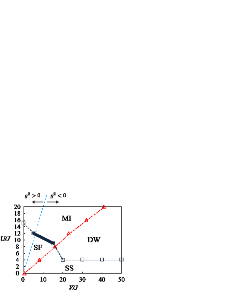
Finally, Fig. A.2 exhibits a phase diagram without rescaling by the mean density . Here, we put, as an example of the large filling, (i.e., average occupation numbers of atoms per site is ten)filling . The coupling constant , , and are not rescaled by the mean density. We found that there are four phases, SF (superuid), MI (Mott insulator), DW (density wave), and SS (supersolid). The DW state is recognized by the AF-type staggererd configuration of the local density average . It is possible that both the quasi-long-range orders of the SF and the diagonal DW order coexist, indicating the supersolid (SS) state. The phase boundaries between SF(SS) and MI(DW) are determined by . On the other hand, the boundaries between SF(MI) and MI(SS) is determined by the specific heat peak.
A.3 Gauge theoretical interpretation including inhomogeneity of density
Let us consider the physical meaning of each phase of the EBHM in the terminology of gauge theory Kogut . The SF phase corresponds to the Higgs phase as the gauge fields has small fluctuations there. On the contrary, the MI corresponds to the confinement phase, as the boson density , which is the electric field in the GHM, has small fluctuations in that phase; therefore, the vector potential fluctuates strongly in the MI. The above identification was verified in Sec. IV through the study on the real-time dynamics of the electric flux.
Next, we consider the DW and SS phases which appear for . The DW phase has a definite density imbalance between even and odd sites., so that the density fluctuation from the mean density is basically small. Therefore, in terms of the gauge theory, the fluctuation of the electric field is small, which means that the DW phase follows the property of the confinement phase. We can say that the DW phase does not have substantial difference from the MI phase from gauge-theoretical point of view. In this sense, the SS state corresponds to the ordinary Higgs phase as the gauge fields have small fluctuations. In Fig. A.1 and Table 2, we show the gauge-theoretical interpretation of the phase diagram of the EBHM.
| EBHM | U(1) GHM | ||
|---|---|---|---|
| MI | Confinement | large | (homogeneous) |
| DW | Confinement | large | |
| SS | Higgs | small | |
| SF | Higgs | small | (homogeneous) |
References
- (1) M. Noack, S. R. Manmana, AIP Conf. Proc. 789, 93-163 (2005).
- (2) M. Troyer and U.-J. Wiese, Phys. Rev. Lett. 94, 170201 (2005).
- (3) I. Bloch, J. Dalibard, and W. Zwerger, Rev. Mod. Phys.80, 885 (2008); M. Lewenstein, A. Sanpera, and V. Ahufinger, Ultracold Atoms in Optical Lattices: Simulating Quantum Many-body Systems (Oxford University Press, Oxford, 2012).
- (4) N. Goldman, G. Juzeliunas, P. Ohberg, and I. B. Spielman, Rep. Prog. Phys. 77 126401 (2014).
- (5) For reviews, see, e.g., U.-J. Wiese, Ann. Phys. 525, 777 (2013); E. Zohar, J. I. Cirac, and B. Reznik, Rep. Prog. Phys. 79, 014401 (2016).
- (6) K. Kasamatsu, I. Ichinose, and T. Matsui, Phys. Rev. Lett. 111, 115303 (2013).
- (7) Y. Kuno, K. Kasamatsu, Y. Takahashi, I. Ichinose, and T. Matsui, New J. Phys. 17, 063005 (2015).
- (8) Y. Kuno, M. Sakane, K. Kasamatsu, I. Ichinose, and T. Matsui, Phys. Rev. A 94, 063641 (2016).
- (9) E. Fradkin and S. H. Shenker, Phys. Rev. D 19, 3682 (1979).
- (10) I. Ichinose and T. Matsui, Mod. Phys. Lett. B 28, 1430012 (2014).
- (11) S. Baier, M. J. Mark, D. Petter, K. Aikawa, L. Chomaz, Z. Cai, M. Baranov, P. Zoller, and F. Ferlaino, Science 352, 201 (2016).
- (12) O. Dutta, M. Gajda, P. Hauke, M. Lewenstein, D.-S. Luhmann, B. A. Malomed, Tomasz Sowioski, J. Zakrzewski Rep. Prog. Phys. 78, 066001 (2015).
- (13) K. Wilson, Phys. Rev. D 10, 2445 (1974); J. Kogut and L. Susskind, Phys. Rev. D 11, 395 (1975).
- (14) S. Chandrasekharan and U. J. Wiese, Nucl. Phys. B 492, 455 (1997).
- (15) Some further advantages of the present approach of identifying the phase of atomic variable to the U(1) gauge field over the quantum link-model is discussed in depth in Sec. I of Ref. Future .
- (16) M. Fattori, G. Roati, B. Deissler, C. D’Errico, M. Zaccanti, M. Jona-Lasinio, L. Santos, M. Inguscio, and G. Modugno, Phys. Rev. Lett. 101, 190405 (2008); S. Müller, J. Billy, E. A. L. Henn, H. Kadau, A. Griesmaier, M. Jona-Lasinio, L. Santos, and T. Pfau, Phys. Rev. A 84, 053601 (2011).
- (17) E. A. Martinez, C. A. Muschik, P. Schindler, D. Nigg, A. Erhard, M. Heyl, P. Hauke, M. Dalmonte, T. Monz, P. Zoller and R. Blatt, Nature(London), 534, 516 (2016).
- (18) A. Bazavov, Y. Meurice, S.-W. Tsai, J. Unmuth-Yockey, and J. Zhang, Phys. Rev. D 92, 076003 (2015).
- (19) V. L. Berezinskii, Sov. Phys. JETP 32, 493(1971); ibid 34,610 (1972); J. M. Kosterlitz and D. J. Thouless, J. Phys C6,1181(1973).
- (20) K. Adcox et al. (PHENIX Collaboration), Nucl.Phys.A 757:184-283, (2005).
- (21) P.G. Kevrekidis, The Discrete Nonlinear Schrödinger Equation (Berlin: Springer) (2009).
- (22) T. Pichler, M. Dalmonte, E. Rico, P. Zoller, and S. Montagero, Phys. Rev. X 6, 011023 (2016).
- (23) A. Sinatra, C. Lobo, and Y. Castin, J. Phys. B At. Mol. Opt. Phys. 35, 3599 (2002); A. Polkovnikov, Phys. Rev. A 68, 053604 (2003); P. B. Blakie, a. S. Bradley, M. J. Davis, R. J. Ballagh, and C. W. Gardiner, Advances in Physics, 57, 363 (2008).
- (24) T. Lahaye, C. Menotti, L. Santos, M. Lewenstein, and T. Pfau, Reports Prog. Phys. 72, 126401 (2009); M. A. Baranov, M. Dalmonte, G. Pupillo, and P. Zoller, Chem. Rev. 112, 5012 (2012).
- (25) S. Inouye, M. R. Andrews, J. Stenger, H.-J. Miesner, D. M. Stamper-Kurn, and W. Ketterle, Nature 392, 151 (1998); C. Chin, et al. Rev. Mod. Phys. 82, 1225 (2010)
- (26) This asymmetric XY model itself is related to a 1D quantum-rotor model and analized numerically in H. Zou, Y. Liu, C. Lai, J. Unmuth-Yockey, L. Yang, A. Bazavov, Z. Xie, T. Xiang, S. Chandrasekharan, S.-W. Tsai, Y. Meurice, Phys. Rev. A 90, 063603 (2014).
- (27) W. Janke, Phys. Rev. B 55, 3580 (1997).
- (28) See, for example, J. B. Kogut, Rev. Mod. Phys. 51, 659 (1979).
- (29) For low density case, D. Rossini and R. Fazio, New J. Phys. 14, 065012 (2012); G. G. Batrouni, V. G. Rousseau, R. T. Scalettar, and B. Gremaud, Phys. Rev. B 90, 205123 (2014).
- (30) K. Kawaki, Y. Kuno, and I. Ichinose, Phys. Rev. B 95, 195101 (2017).
- (31) L. P. Pitaevskii and S. Stringari, Bose-Einstein Condensation (Oxford University Press, Oxford, 2003); J. Rogel-Salazar, Eur J Phys 34, 247 (2013).
- (32) F. Hebenstreit, J. Berges, and D. Gelfand, Phys. Rev. D 87, 105006 (2013); V. Kasper, F.Hebenstreit, M.Oberthaler, and J.Berges, Phys. Lett. B 760, 742 (2016).
- (33) P. Wurtz, T. Langen, T. Gericke, A. Koglbauer, and H. Ott, Phys. Rev. Lett. 103, 080404 (2009).
- (34) J. Smit, Introduction to Quantum Fields on a Lattice (Cambridge Lecture Notes in Physics).
- (35) D. Banerjee, M. Dalmonte, M. Muller, E. Rico, P. Stebler, U.-J. Wiese, and P. Zoller, Phys. Rev. Lett. 109, 175302 (2012).
- (36) J. Schwinger, Phys. Rev. 82, 664 (1951).
- (37) Y. Kuno, K. Suzuki, and I. Ichinose, Phys. Rev. A 90, 063620 (2014).
- (38) Strictly speaking, the correct expression is , which is replaced by the integral and the compactification
- (39) In the present discussion, we assume that a long-range order of the Ising-type fluctuations of does not exist. If this long-range order exists, the system is in the density-wave. In this phase, the finite ‘magnetization’ exists.
- (40) This enhancement of the SF is actually observed by the SSE-quantum MC simulation of the EBHM at low fillings. See Ref. Kawaki
- (41) N. Metropolis, A. W. Rosenbluth, M. N. Rosenbluth, A. M. Teller, E. Teller, J. Chem. Phys. 21, 1087 (1953).
- (42) In general, it is difficult to carry out a numerical simulation for large filling beyond mean-field theory due to enormous consumption of computer memory.