Quantum stochastic transport along chains
Abstract
The spreading of a particle along a chain, and its relaxation, are central themes in statistical and quantum mechanics. One wonders what are the consequences of the interplay between coherent and stochastic transitions. This fundamental puzzle has not been addressed in the literature, though closely related themes were in the focus of the Physics literature throughout the last century, highlighting quantum versions of Brownian motion. Most recently this question has surfaced again in the context of photo-synthesis. Here we consider both an infinite tight-binding chain and a finite ring within the framework of an Ohmic master equation. With added disorder it becomes the quantum version of the Sinai-Derrida-Hatano-Nelson model, which features sliding and delocalization transitions. We highlight non-monotonic dependence of the current on the bias, and a counter-intuitive enhancement of the effective disorder due to coherent hopping.
Introduction
A prototype problem in Physics is the dynamics of a particle along chain that consists of sites. If the dynamics is coherent one expects to observe ballistic motion and Bloch oscillations Hartmann_korsch_2004, while for stochastic dynamics one expects to see diffusion and drift. In the presence of disorder, additional fascinating effects emerge: an Anderson localization transition in the coherent problem, and a Sinai-Derrida sliding transition in the stochastic problem. In practical applications the particle can be an exiton dubin2006macroscopic; nelson2018coherent; dekorsy2000coupled. Past literature regarding quantum spreading in chains, MadhukarPost1977; Weiss1985; Kumar1985; Dibyendu2008; Amir2009; lloyd2011quantum; Moix_2013; CaoSilbeyWu2013; Kaplan2017ExitSite; Kaplan2017B, including publications that address the photo-synthesis theme amerongen2000photosynthetic; ritz2002quantum; FlemingCheng2009; plenio2008dephasing; Rebentrost_2009; Alan2009; Sarovar_2013; higgins2014superabsorption; celardo2012superradiance; park2016enhanced, were focused mainly on the question how noise and dissipation affect coherent transport. In a sense, our interest is in the reversed question.
In the present work we assume independent mechanisms for stochastic asymmetric (dissipative) transitions, and for coherent hamiltonian (conservative) transitions. Such setup is not common: the standard models do not allow to tune on and off the two mechanisms independently. The question arises how the two mechanisms affect each other. Can we simply “sum up” known results for stochastic transport with known results for coherent motion in noisy environment? We shall see that the answer is not trivial. The main surprises come out once we take into account the presence of disorder (see below). An optional way to phrase the question: what is the quantum version of the prototype stochastic problem that is known in the literature as random walk in random environment. As we know from the above cited works, due to disorder, the stochastic dissipative dynamics is not merely a simple minded Brownian motion. We would like to know whether coherence has any implication on the predicted disorder-related crossovers.
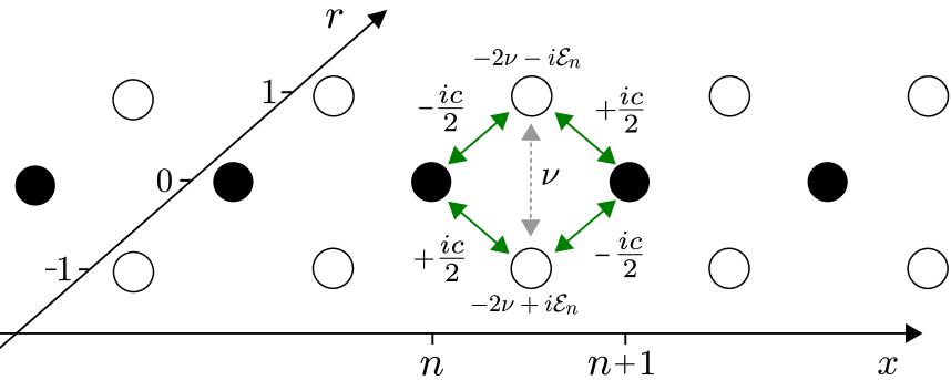
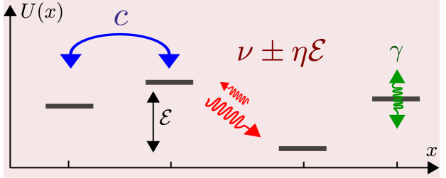
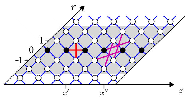
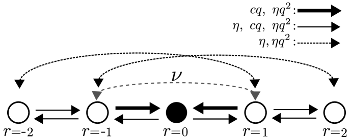
We consider a chain whose sites are labeled by . The particle, or the exiton, can move from site to site (near neighbor transitions only). The transitions are determined by two major parameters: the hopping frequency () that controls the coherent hopping; and the fluctuations intensity () that controls the environmentally-induced stochastic transitions. At finite temperature there is also a dissipation coefficient that is responsible for the asymmetry of the stochastic transitions. On top we might have bias (), on-site noisy fluctuations (), and different types of disorder. The model is illustrated in Fig. 1.
The dynamics is governed by a master equation for the probability matrix
| (1) |
where the dissipators and are due to the interaction with the environment. They are responsible for the stochastic aspect of the dynamics. The Hamiltonian contains an on-site potential , and a sum over hopping terms . Accordingly it takes the form
| (2) |
where is the momentum operator. The unit of length is the site spacing ( is an integer), and the field is
| (3) |
In the absence of stochastic terms, coherent transport in ordered chain leads to ballistic motion (without bias) and exhibits Bloch-oscillations (with bias). In disordered chain the spreading is suppressed due to Anderson-localization. The effect of noise and dissipation on coherent transport due to has been extensively studied. In the Caldeira-Leggett model Caldeira1983; CALDEIRA1983374 the interaction is with homogeneous fluctuating environment, leading to Brownian motion with Gaussian spreading. If the interaction is with non-homogeneous fluctuating environment (short spatial correlation scale) the spreading is the sum of a decaying coherent Gaussian and a scattered Stochastic Gaussian Cohen1997. The tight binding version of this model has been studied in EspositoGaspard2005. It has been found that the decoherence and the stochastic-like evolution are dictated by different bands of the Lindblad -spectrum that correspond, respectively, to the dephasing and to the relaxation rates in NMR studies of two-level dynamics.
In the other extreme of purely stochastic dynamics, ignoring quantum effects, the disordered model, aka random walk in random environment, has been extensively studied by Sinai, Derrida, and followers Dyson1953; Sinai1983; DerridaPomeau1982; Derrida1983; havlin1987diffusion; Bouchaud1990; BOUCHAUD1990a. Without bias the spreading becomes sub-diffusive, while above some critical bias the drift-velocity becomes finite, aka sliding transition. Strongly related is the transition from over-damped to under-damped relaxation that has been studied for a finite-size ring geometry HurowitzCohen2016; HurowitzCohen2016a. The latter involves delocalization transition that has been highlighted for non-hermitian Hamiltonians in the works of Hatano, Nelson and followers Hatano1996; Hatano1997; Hatano1998; LubenskyNelson2000; LubenskyNelson2002; Amir2015; Amir2016; Shnerb99.
One should realize that the two extreme limits of coherent and stochastic spreading have to be bridged within the framework of a model that includes an term, not just an term. Furthermore, a proper modeling requires the distinction between two types of Master equations. In one extreme we have the Pauli version. Traditionally this version is justified by the secular approximation that assumes weak system-bath interaction. In the other extreme we have the Ohmic version that assumes short correlation time. The so called “singular coupling limit” can be regarded as an optional way to formalize the short correlation time assumption Rivas2012. Clearly in the mesoscopic context it is more appropriate to adopt the Ohmic version, and regard the Pauli version of the dissipator as a formal approximation.
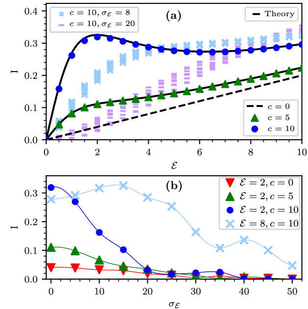
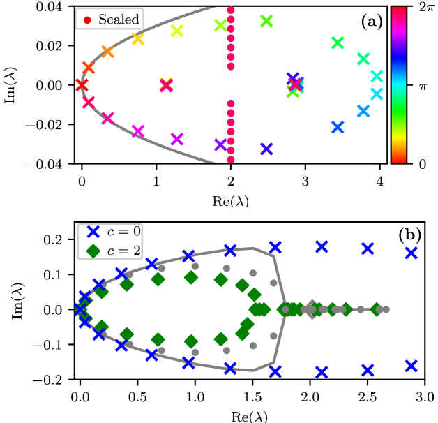
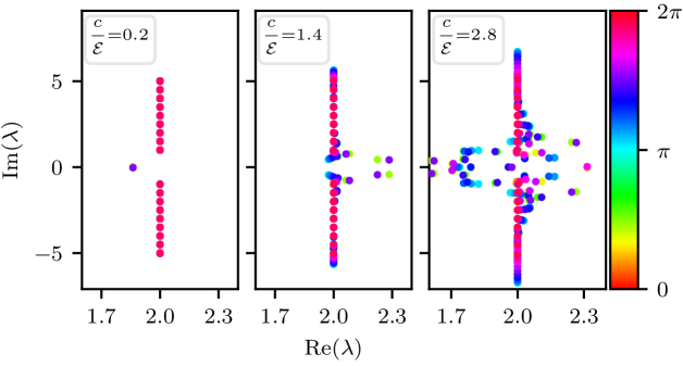
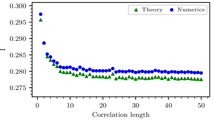
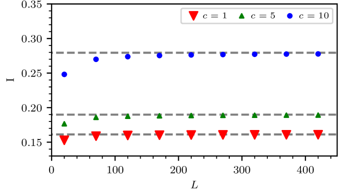
Outline.– The model is presented in terms of an Ohmic master equation. The units of time are chosen such that the basic model parameters are and the strength of the disorder . The interest is in the diffusion coefficient , the -induced drift velocity , the implied non equilibrium steady state (NESS) current for a ring of length , and the associated Lindblad -spectrum. The latter is determined via , which provides both the relaxation-modes and the decoherence-modes. In particular we observe that the NESS current depends non-monotonically on the bias (Fig. 2a), and that surprisingly it can be enhanced by disorder (Fig. 2b). In a disordered ring, counter-intuitively, relaxation modes become over-damped if coherent transitions are switched on (Fig. 3).
Results
The model.– The isolated chain is defined by the Hamiltonian equation (2), that describes a particle or an exiton that can hop along a one-dimensional chain whose sites are labeled by . The field might be non-uniform. For the average value of the field we maintain the notation , while the random component is distributed uniformly (box distribution) within . We regard each pair of neighboring sites as a two-level system S (1). Accordingly we distinguish between two types of terms in the master equation: those that originate from temporal fluctuations of the potential (dephasing due to noisy detuning), and those that are responsible to stochastic transition between the sites (incoherent hopping). The latter are implied by the replacement at the pertinent bonds, where is a bath operator that is characterized by fluctuation intensity , and temperature . Hence the system bath coupling term is , where and . The baths of different bonds are uncorrelated, accordingly the bond-related dissipator takes the form
| (4) |
where is the friction coefficient, and
| (5) |
The friction terms represent the response of the bath to the rate of change of the . Note that for getting the conventional Fokker-Planck equation the system-bath coupling term would be , and would become the velocity operator. Here we assume interaction with local baths that in general might have different temperatures. See Methods for some extra technical details regarding the master equation, the nature of the disorder, and the handling of the periodic boundary conditions for the ring configuration.
Pauli-type dynamics.– For pedagogical purpose let us consider first a uniform non-disordered ring without coherent hopping. Furthermore, let us adopt the simplified Pauli-like version of the dissipator (see Methods). Consequently the dynamics of the on-site probabilities decouples from that of the off-diagonal terms. Namely, one obtains for the probabilities a simple rate equation, where the transition rates between sites are
| (6) |
in agreement with Fermi-golden-rule (FGR). Note that in leading order as expected from detailed balance considerations. It follows that the drift velocity and the diffusion coefficient are:
| (7) | |||||
| (8) |
Consequently one finds two distinct sets of modes: the stochastic-like relaxation modes that are implied by the rate equation for the probabilities, and off-diagonal decoherence modes. The latter share the same decay rate , where stands for optional extra off-diagonal decoherence due to on-site fluctuations. An evolving wavepacket S (3) will decompose into coherent decaying component that is suppressed by factor , and an emerging stochastic component that drifts with velocity and diffuse with coefficient .
Full Ohmic treatment.– The state of the particle in the standard representation is given by . The master equation, equation (1) with equation (4), couples the dynamics of the on-site probabilities to that of the off-diagonal elements . The generator can be written as a sum of several terms S (5):
| (9) |
Each term is a super-matrix that operates on the super vector . The first two terms and arise from the Hamiltonian equation (2). The term arise from the first term of equation (4), which represent noise-induced transitions. The remaining two friction-terms (proportional to ) arise from equation (5), and correspond to the two terms in the Hamiltonian.
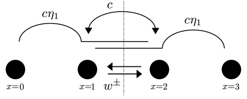
A schematic representation of and the couplings is given in Fig. 4. The coherent hopping that is generated by couples to and to , while contribute “on-site” potential. The noise operator include the Pauli-terms that were discussed previously, and an additional term that couples the elements. Together with the friction operator , the Pauli terms induce the asymmetric stochastic transitions of equation (6) along . The second friction term consists of non-Pauli terms that allow extra -type couplings, and in particular extra transitions within the strip .
The spectrum for a non-disordered ring.– For a non-disordered ring the super-matrix is invariant under -translations, and therefore we can switch to a Fourier basis where the representation is . Due to Bloch theorem, the matrix decompose into -blocks in this basis. Thus in order to find the eigenvalues and the corresponding eigenmodes we merely have to handle a one dimensional tight binding lattice. See Methods. A representative spectrum is provided in Fig. 3a. Consider first the eigenstates. For the -dependent couplings are zero. For infinite temperature () the only non-zero coupling is between due to a non-Pauli term in equation (33). Consequently the block contains the NESS (which is merely the identity matrix in the standard basis), along with a pair of non-trivial decoherence modes , and a set of uncoupled decoherence modes . The corresponding eigenvalues (for ) are:
| (10) | |||||
| (11) | |||||
| (12) |
The modes become over-damped for small bias, while the decoherence modes are always under-damped. Considering the dependence of the eigenvalues we get several bands, as illustrated in Fig. 3a. Our interest below is in the relaxation modes that are associated with , and determine the long time spreading.
The NESS.– At finite temperature () there are extra couplings that lead to a modified NESS. In leading order the NESS eigenstate is with
| (13) |
Reverting back to the standard representation we get
| (14) |
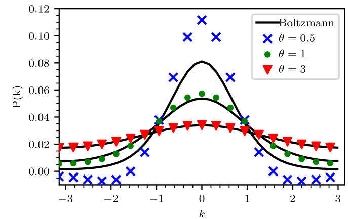
From this we can deduce the steady state momentum distribution S (5), namely, . The result in leading order is
| (15) |
For this expression is consistent with the canonical expectation .
The current.– For non-zero field () the NESS momentum distribution is shifted. The expression for the current operator is complicated S (2), but the net NESS current comes out a simple sum of stochastic and coherent terms:
| (16) | |||||
| (17) |
We shall further illuminate the physical significance of the second term below. In contrast with the stochastic case, the drift current might be non-monotonic in , see Fig. 2a. Furthermore, there is a convex range where the second derivative of is positive.
The convexity of the current in some range, implies a counter intuitive effect: current may become larger due to disorder. The argument goes as follows: Assume that the sample is divided into two regions, such that is constant in each region, but slightly smaller (larger) than in the first (second) region. Due to the convex property it is implied that the current will be larger. Extending this argument for a general non-homogeneous (i.e. disordered) field, with the same average bias , we expect to observe a larger NESS current. This is indeed confirmed in Fig. 2a, while additional examples are given and discussed quantitatively in S (6).
The Diffusion.– An optional way to derive equation (17) is to expand in , to obtain . The second order term gives the diffusion coefficient. Namely,
| (18) |
It is therefore enough to determine via second order perturbation theory with respect to the eigenstates. To leading order in , a lengthy calculation leads to a result that is consistent with the Einstein relation, namely
| (19) |
Thus, to leading order, is given by equation (8), multiplied by the expression in the square brackets in equation (17). We see that with coherent transitions, for zero bias, this expression takes the form , where . The latter can be interpreted as a Drude-type result , with relaxation time and mean free path . A similar expression has been obtained in MadhukarPost1977; EspositoGaspard2005 for a chain with noisy sites. In the other extreme of large bias equation (8) implies that . This result, like the Drude result, can be regarded as coming from FGR transitions. But now the transitions are between Bloch site-localized states. Namely, we have hopping between neighboring sites (), with rate of the transitions () that is suppressed by a factor . The suppression factor reflects the first-order-perturbation-theory overlap of Bloch-localized wavefunctions. To summarize: we can say that exhibits a crossover from Drude-type transport to hopping-type transport as the field is increased.
In fact we can proceed beyond leading order, and calculate up to second order in , see S (5). Here we cite only the zero bias result:
| (20) |
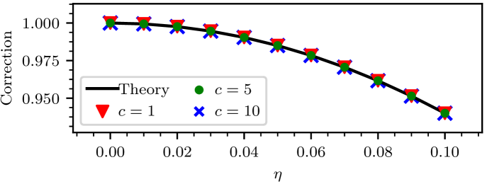
In view of the Drude picture this result is surprising. Namely, one would expect to be replaced by , and hence one would expect the replacement due to the narrowing of the momentum distribution, see Methods. However the current result indicates that the leading correction is related to a different mechanism. Indeed, using a semiclassical perspective, the coupling to the bath involves a factor, see Methods. The zero order diffusion with rate arises due to stochastic term in the equation of motion for that involves a factor, Consequently, due to thermal averaging, , which explains, up to a factor of 2, the third term in equation (20). We have repeated this calculation also for a Caldeira-Leggett dissipator, and also for an dissipator. For the former the expected correction to appears, but has a different numerical factor, while for the latter the correction comes out with an opposite sign. We can show analytically that the discrepancies are due to the modification of the correlation time qssXs-prep.
Disordered ring.– The so called stochastic field is responsible for the asymmetry of the incoherent transitions. Following Sinai we assume that it has a random component that is (say) box-distributed. From the works of Sinai and Derrida Sinai1983; DerridaPomeau1982; Derrida1983 we expect a sliding transition as exceeds a critical value of order . Strongly related is the delocalization transition Hatano1996; Hatano1997; Hatano1998; Amir2015; Amir2016; HurowitzCohen2016 for which the critical value is smaller by a numerical factor. Disregarding this factor we expect
| (21) |
In the purely stochastic model, for the relaxation is expected to be under-damped due to a delocalization transition that leads to the appearance of complex eigenvalues at the vicinity of .
The question arises how this transition is affected by quantum coherent hopping. The naive expectation would be to witness a smaller tendency for localization in the relaxation-spectrum because we add coherent bypass that enhances the transport. But surprisingly the numerical results of Fig. 3b show that the effect goes in the opposite direction: for non-zero , some eigenvalues become real, indicating stronger effective disorder.
Enhanced effective disorder.– We turn to provide an explanation for observing enhanced effective disorder due to coherent hopping. On the basis of the non-disordered ring analysis, the relaxation modes occupy mostly the diagonals of , and therefore it makes sense to exclude couplings to the higher diagonals. We verify that this does not change the qualitative picture in Fig. 3b (gray vs green symbols). The effect of the band is to introduce virtual coherent transitions between diagonal elements S (7). Hence we end up with an effective single-band stochastic equation with transition rates
| (22) | |||||
| (23) |
The disorder that is associated with is hermitian, namely, it does not spoil the symmetry of the transitions, it merely implies that the we have a tight binding model with random couplings that have some dispersion . This is known as resistor network (RN) disorder. In contrast, the term induces asymmetric transitions. This type of non-hermitian Sinai-type disorder is characterized by the dispersion . The latter translates after non-hermitian gauge transformation to (hermitian) diagonal disorder, with ill-defined boundary conditions. The procedure to handle both types of disorder has been discussed in HurowitzCohen2016 following Hatano1997. One defines an hermitian RN matrix by setting in equation (22). The RN matrix has a real spectrum with eigenstates that are characterized by inverse localization length that is dominated by the RN-disorder, namely, . Adding back the field , the eigenstates remain localized (with real eigenvalues) only in regions where localization is strong enough, that is, . Estimating , see S (7) for an explicit expression, we deduce that the additional RN disorder is responsible for the observed numerical result.
The Wannier-Stark Ladder.– We shift our attention to the full Lindblad spectrum. In the absence of coupling to the bath, the eigenstates of the Hamiltonian equation (2) are Bloch localized. Each eigenstate occupies a spatial region , and the corresponding eigen-energies form a ladder with spacing , that reflects the frequency of the Bloch oscillations. Weak coupling to the bath leads to damping of the Bloch oscillations. This is reflected by the Lindblad spectrum. For the modes we have obtained equation (12), where we see that the eigenvalues acquire a real part, but maintain the ladder structure. But for non-zero the term couples the modes to the perturbation that is created at the region by , see equation (31) and equation (33) of the Methods. This results in a deformation of the ladder. Namely, the ladder consists of bands, and the number of bands that are deformed equals the Bloch localization length. See Fig. 5.
Regime diagram.– We would like to place our results in the context of the vast quantum dissipation literature. The prototype model of Quantum Brownian Motion (QBM), aka the Caldeira-Leggett model, involves coupling to a single bath that exerts a fluctuating homogeneous field of force. In the classical framework it leads to the standard Langevin equation
| (24) |
and equation (1) becomes the standard Fokker Planck equation. In the tight-binding framework we have the identification , where is the lattice constant. The standard QBM model features a single dimensionless parameter, the scaled inverse temperature , which is the ratio between the thermal time and damping time . In the lattice problem we can define two dimensionless parameters
| (25) | |||||
| (26) |
Accordingly . Note that in our model we set the units such that , hence, disregarding factor, our scaled friction parameter is the same as .
The standard analysis of QBM HakimAmbegaokar1985 reveals that quantum-implied memory effects are expressed in the regime , where a transient spreading is observed in the absence of bias, followed by diffusion. Most of the quantum dissipation literature, regarding the two-site spin-boson model LeggettEtAlDynamicsTwoLevel1987 and regarding multi-site chains aslangul1986quantum; AslangulPeriodicPotential1987, is focused in this low temperature regime, where significant deviations from the classical predictions are observed for large of order unity. In contrast, our interest is in the regime.
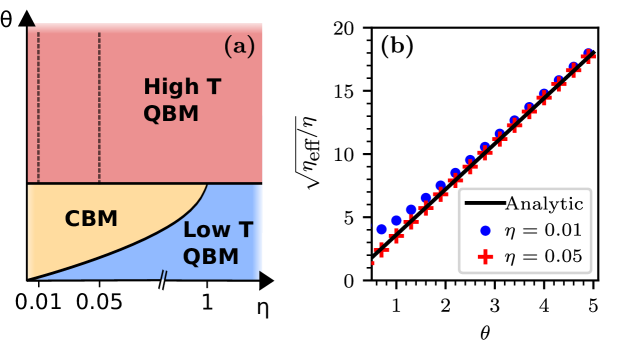
Our regime diagram Fig. 6 is roughly divided into two regions by the line . Along this line the thermal de-Broglie wavelength of the particle is of order of the lattice constant, hence it bears formal analogy to the analysis of QBM in cosine potential Fisher1985QuantumBrownianPeriodic, where it marks the border to the regime where activation mechanism comes into action. In our tight binding model we have a single band, hence transport via thermal activation is not possible. Rather, in the regime, where , the momentum distribution within the band is roughly flat, and the drift is dictated by equation (17), that is,
| (27) |
where for weak field. The low temperature regime has not been addressed in this work, because the Ohmic master equation fails to reproduce canonical equilibration in this regime (see Methods). Still we would like to illuminate what we get (not presented) if this aspect is corrected. In the regime the momentum distribution becomes much narrower (only low energy momenta are populated) and therefore as implied by equation (24). This we call Classical-like Brownian motion (CBM) regime. Once the coupling to the bath is not the simple -coupling of the Caldeira-Leggett model, a numerical prefactor is expected (see Methods for detailed argument).
Discussion
There is a rich literature regarding Quantum Brownian motion (see Schwinger1961; HakimAmbegaokar1985; GRABERT1988115; HanggiQBM2005 and references within). In the condensed matter literature it is common to refer to the Caldeira-Leggett model Caldeira1983; CALDEIRA1983374, where the particle is linearly coupled to a bath of harmonic oscillators that mimic an Ohmic environment. Some works study the motion of a particle in a periodic potential, possibly with bias, aka washboard potential Schmid1983; Fisher1985QuantumBrownianPeriodic; Fisher1985QuantumBrownianPeriodic; AslangulPeriodicPotential1987, while other refer to tight binding models Weiss1985; aslangul1986quantum; Weiss1991 as in this work. The focus in those papers is mostly on non-Markovian effects: at low temperatures the fluctuations are not like “white noise”, and are dominated by a high frequency cutoff . Consequently the handling of long-time correlations becomes tricky. In this context the low temperature dependence of the diffusion and the mobility is modified for and .
The line of study in the above models has assumed that the fluctuations that are induced by the bath are uniform in space. In some other works the dynamics of a particle that interacts with local baths has been considered. In such models the fluctuations acquire finite correlation length in space Cohen1997; MadhukarPost1977; Kumar1985; EspositoGaspard2005; Dibyendu2008; Amir2009; lloyd2011quantum; Moix_2013; CaoSilbeyWu2013; Moix_2013; Kaplan2017ExitSite; Kaplan2017B. The extreme case, as in this work, are tight binding models where the coupling is to uncorrelated baths that seat on different sites or bonds. Studies in this context assume bath that are connected at the end points znidaricOpenQuantumChain2010, or baths that act as noise source MadhukarPost1977. Ref. EspositoGaspard2005 has analyzed the spectral properties for a chain with noisy sites, Ref. Amir2009 has considered colored noise sources strongly coupled to each site, Ref. EislerCrossoverBallistiDiffusiveQuantum_2011 has considered noisy transitions on top of coherent transitions, Ref. znidaricDisorderDephasing2013 has considered transport in the presence of dephasing and disorder, Ref. Moix_2013 has considered numerically transport properties of a noisy system with static disorder, and Han_local_bath_diffusion_2018 has addressed some bounds in the absence of disorder. The basic question of transport in a tight-binding models has resurfaced in the context of excitation transport in photosynthetic light-harvesting complexes amerongen2000photosynthetic; ritz2002quantum; plenio2008dephasing; FlemingCheng2009; Rebentrost_2009; Alan2009; Sarovar_2013; higgins2014superabsorption; celardo2012superradiance; park2016enhanced.
It is quite surprising that all of the above cited works have somehow avoided the confrontation with themes that are familiar from the study of stochastic motion in random environment. Specifically we refer here to the extensive work by Sinai, Derrida, and followers Dyson1953; Sinai1983; DerridaPomeau1982; Derrida1983; havlin1987diffusion; Bouchaud1990; BOUCHAUD1990a, and the studies of stochastic relaxation HurowitzCohen2016; HurowitzCohen2016a which is related to the works of Hatano, Nelson and followers Hatano1996; Hatano1997; Hatano1998; Shnerb99; LubenskyNelson2000; LubenskyNelson2002; Amir2015; Amir2016; HurowitzCohen2016; HurowitzCohen2016a. Clearly we have here a gap that should be bridged.
In this article we have studied transport properties along a chain taking into account several themes that have not been combined in past studies: (a) The baths on different bonds are not correlated in space; (b) The baths are not just noise - the temperature is high but finite; (c) Without coherent hopping it is the Sinai-Derrida-Hatano-Nelson model which exhibits sliding and delocalization transitions; (d) Without baths it is a disordered chain with Anderson localization; (e) The bias might be large such that Bloch dynamics is reflected.
The “small” parameter in our analysis is the inverse temperature. The following observations have been highlighted: (1) The NESS current is the sum of stochastic and quasi-coherent terms; (2) It displays non-monotonic dependence on the bias, as shown in Fig. 2, due to crossover from Drude-type to hopping-type transport; (3) Disorder may increase the current due to convex property; (4) The interplay of stochastic and coherent transition is reflected in the Lindblad spectrum; (5) In the presence of disorder the quasi-coherent transitions enhance the localization of the relaxation modes. Thus, with regard to the Sinai-Derrida sliding transition, and the strongly related Hatano-Nelson delocalization transition, we find that adding coherent transitions “in parallel” have in some sense opposite effects: on the one hand they add bypass for the current (point (1) above), but on the other hand they enhance the tendency towards localization (point (5) above). Some of our results might be relevant to studies of optimal transport efficiency R (1, 2) and the quantum Goldilocks effect R (3).
Methods
Master equation for disordered chain.–
A pedagogical presentation of the procedure for the construction of an Ohmic master
equation for a two site system, and then for a chain, is presented in S (1).
Each bond has a different bath, and therefore can experience different temperature and friction.
Accordingly we can have disorder that originates either from the Hamiltonian
(say random as assumed in the main text),
or from having different baths (random or random ).
This extra disorder can be incorporated in a straightforward manner,
and does not affect the big picture.
Thermalization.– The Ohmic master equation for a Brownian particle, if the coupling to the bath were , is the standard Fokker-Plank equation. It leads to canonical thermal state for any friction and for any temperature. This is not the case for a discrete two level system. The agreement with the canonical result is guaranteed only to first order in . This is reflected in equation (6). The same applies for a chain. Note that in this sense the Ohmic approximation is very different from the secular or Pauli approximation Breuer2002, or specially constructed Davies Liovillian davies1976quantum, that guarantee canonical thermalization.
It is important to identify the “small parameter” that controls
the deviation from canonical thermalization. The standard coupling via
induce transitions between neighboring momenta, and therefore the small parameter
is , where the level spacing goes to zero in the limit.
But for local baths, the coupling is to scatterers,
that create transitions to all the levels within the band.
Therefore the small parameter in the absence of bias is .
This assertion is confirmed numerically by inspection of the equilibrium
momentum distribution , see S (5).
We conclude that in the regime of interest ()
the Ohmic master equation can be trusted, while for lower temperatures
we have to “correct” it.
For the two site system the “corrected” equation is the Bloch equation,
where the ratio of the rates is in agreement with detailed balance
(not just in leading order in ). For a chain, we cannot justify the secular approximation,
and therefore the correction procedure is ill defined.
The friction coefficient.–
In the Caldeira-Leggett model for Brownian particle,
with interaction term ,
the bath induced fluctuations
are determined by a coupling constant ,
and by the bath temperature ,
such that at high temperatures the intensity
of the fluctuations is .
The parameter is defined such that the
friction coefficient in equation (24) equals .
A straightforward generalizations Cohen1997
shows that for interaction with local baths
,
with ,
the effective friction coefficient is
.
For homogeneous distribution of local baths that have
the same , the friction coefficient becomes -independent.
In the model under consideration the coupling
to the baths is ,
where labels the sites.
Disregarding commutation, it can be written as
,
where the -s are site localized.
It follow that the effective friction coefficient is
momentum dependent, namely
.
But for equilibration in the regime
only low momenta are important
hence we expect, up to numerical prefactor
to observe .
The failure to observe this result is due to improper
thermalization, as discussed in a previous paragraph.
Positivity.– Irrespective of , there is another complication with the Ohmic master equation. If the temperature is low (small ) the relaxation may lead to a sub-minimal wavepacket that violates the uncertainty principle. This reflects the observation that the Ohmic master equation is not of Lindblad form, and violates the positivity requirement. The minimal correction required to restore positivity is to couple to an extra noise source of intensity
| (28) |
This term is essential in the low temperature regime.
We have verified numerically that the extra noise term can be neglected
in the high temperature regime where our interest is focused.
On-site dissipators.–
The model of EspositoGaspard2005 combines Hamiltonian term
with dissipator of the type
that originates from couplings via ,
where .
Such dissipator leads to off-diagonal dephasing
that is generated by terms,
and therefore excludes the possibility for inter-site stochastic transitions.
Similar remark applies to the familiar Caldeira-Leggett model
of Quantum Brownian motion Caldeira1983, where the coupling is via .
Namely, it is a single bath that exerts a fluctuating homogeneous force
that affects equally all the sites, as in aslangul1986quantum.
In our model the dissipation effect is local: many uncorrelated local baths.
Pauli dissipator.– A conventional Pauli-type dissipator is obtained if we drop some of the terms in the Ohmic dissipator of equation (4). Namely,
| (29) |
The transition rates between sites, ,
are in agreement with FGR.
For completeness, we added here a term that represents
optional off-diagonal decoherence due to on-site noise.
Ring configuration.–
For numerical treatment, and for the purpose of studying relaxation dynamics, we close the chain into a ring.
This means to impose periodic boundary conditions.
With uniform field , one encounter a huge potential drop at the boundary.
To avoid this complication we assume that the boundary bond has an infinite temperature,
hence the formation of a stochastic barrier is avoided,
and the circulation of the stochastic field (aka affinity) becomes as desired.
In the analytical treatment of a clean ring we assume
that , and and in the master equation are all uniform,
such that invariance under translation is regained.
This cheat is valid for large ring if is banded,
reflecting a finite spatial correlation scale.
See numerical verification in S (2).
The Bloch eigenstates of a clean ring.– The super-operator in the Bloch basis, decomposes into Blocks. Each block can be written as a sum of terms, as in equation (9), that operate over a one dimensional tight binding lattice. In this representation the coherent dynamics is generated by
| (30) | |||||
| (31) |
where . For the induced stochastic transitions we have
| (33) | |||||
where the last term is non-Pauli. The Pauli-type friction term takes the form:
| (34) |
And the additional friction terms are:
| (37) | |||||
Note that the zero eigenvalue belongs to the block.
Some more details are provided in S (5).
Diffusion at finite temperature.– The Drude type term in the expression for the diffusion equation (20) is up to numerical prefactor , where for uniform momentum distribution. At finite temperature this distribution equation (15) is not uniform. Here we consider zero bias and get
| (38) |
where , and recall that . The analytical calculation in S (5) leads to a different result which implies that the expression in the square brackets should be replaced by , which means that the relevant dimensionless parameter is and not . Fig. S4 of S (5)b confirms this statement.
Acknowledgment.–
This research was supported by the Israel Science Foundation (Grant No.283/18).
References
- R (1) Optimal transport in one-dimensional infinite chains has been studied in MadhukarPost1977; Kumar1985; Weiss1985; plenio2008dephasing; Amir2009; Rebentrost_2009.
- R (2) Optimal transport in one-dimensional chains with “exit site” has been studied in Kaplan2017ExitSite; Kaplan2017B; CaoSilbeyWu2013
- R (3) The term quantum Goldilocks effect has been suggested in lloyd2011quantum, for the idea that natural selection tends to drive quantum systems to the degree of optimal quantum coherence for transport.
- S (1) See SM sections 1 and 2 for pedagogical presentation of the procedure for the construction of an Ohmic master equation for 2 a site system and for a chain.
- S (2) See SM section 3 for an explicit expression for the current operator.
- S (3) See SM section 4 for pedagogical summary regarding spreading, following Cohen1997.
- S (4) See SM section 4 for technical summary of the procedure for finding the eigenvalues of a master equation with a Pauli-type dissipator. It follows EspositoGaspard2005, but here we include additional stochastic transitions in “parallel” to the coherent hopping, and incorporate also the bias within a first order treatment.
- S (5) See SM sections 5-7 for technical details regarding the procedure for finding the eigenmodes of the Ohmic master equation, including explicit expressions for the related terms in the Fourier representation, numerical verification for momentum thermalization, and derivation of the associated -related correction for the diffusion coefficient.
- S (6) See SM section 3 for extra numerics that concerns the calculation of the current for a disordered chain, and the manifestation of the convex property.
- S (7) See SM section 8 for technical details regarding the derivation of the effective disorder that emerges in the reduced rate equation due to virtual coherent transitions.
Quantum stochastic transport along chains
Dekel Shapira, Doron Cohen
(Supplementary Material)
1 Ohmic dissipator for a two site system
Consider a two site system with Hamiltonian and an Ohmic bath of temperature that induces a fluctuating force of intensity , and system-bath interaction term . The master equation acquire a dissipation term
| (S-1) |
where , and . An extra noise source can be added in order to make the right hand side “positive” in the Lindblad sense:
| (S-2) |
The “minimal correction” that is needed is to set , and then the expression can be written in the Lindblad form
| (S-3) | |||||
| (S-4) | |||||
| (S-5) |
where the Lamb-shift term can be absorbed into the system Hamiltonian. For two site system with
| (S-6) |
and coupling , one has , and the Lamb-shift is zero. The Lindblad generator is
| (S-7) |
The transition rates between the sites are:
| (S-8) | |||
| (S-9) |
A secular-like (Pauli) version of the dissipator is obtained by expanding and keeping only the Lindblad terms with and . Namely,
| (S-10) | ||||
where the last term represents excess noise due to noisy detuning (see below). The mixed terms that have been omitted affect only the decoherence of the off-diagonal terms, and not the rate of transitions between sites. In the Bloch-vector representation the precessing component of the “spin” decays only in the direction in the Ohmic version, and isotropically in the Pauli version. In some sense the dissipation in the Pauli version assumes two independent baths at each bond. If we assume that the detuning is fluctuating with intensity , so that , then an additional term appears, that has the form of Eq. (S-1) with the substitution , and .
2 Ohmic dissipator for a chain
The Hamiltonian of the chain is
| (S-11) |
where is the displacement operator, and . In general the field , as well as the hopping frequencies (), and temperatures might be non-uniform. The interaction with a bath-source that induces non-coherent transitions at a given bond is obtained by the replacement . The baths of different bonds are uncorrelated. Accordingly the dissipation term in the Master equation takes the form
| (S-12) |
where the coupling to the baths is via the operators
| (S-13) | ||||
| (S-14) |
And the Lindblad correction term:
| (S-15) |
with intensity . Such term has negligible effect in the high temperature regime (). Optionally we can add terms that reflect fluctuations of the field. At a given bond it is obtained by the replacement , where represents fluctuations of intensity . The implied coupling operators are
| (S-16) | |||||
| (S-17) |
3 Expression for the current
For generality of the treatment we allow the temperature to be bond dependent, then so that the Lindblad generators are , and
| (S-18) |
The time dependence of an expectation value is given by the adjoint equation:
| (S-19) |
where
| (S-20) |
Partitioning the system at the -th bond, the current flowing from left to right is defined by , with
| (S-21) |
We note that although the original Hamiltonian allows only near-neighbor hopping, the master equation allows also “double hopping” due to the terms. Accordingly the expression for the current operator has several non-trivial terms. Applying Eq. (S-19) the current is:
| (S-22) | ||||
| (S-23) | ||||
|
|
(S-24) | |||
| (S-25) | ||||
| (S-26) |
where the extra terms are of order , and are negligible for the NESS current. If the field is non-uniform, then one needs to make the replacement . Disregarding the distinct elements of the current are coherent hopping, stochastic hopping and stochastic-assisted coherent hopping. These are pictured in Fig. S1.
Current in disordered system.– In Fig. S2 we display results for the NESS current, calculated for a disordered sample. If the spatial correlation scale of the disorder is large, the ring can be regarded as composed of several segments connected in series. Then the analytical estimate for the current would be
| (S-27) |
which reduce to for a uniform field. The function is provided by Eq. (17), and the above analytical estimate implies what we call convex property. Using this formula we can explain why disorder can lead to increase of the current as in Fig. 2. The accuracy of this formula, that assumes a large spatial correlation scale, is tested against the correlation scale in Fig. S2.
4 Spreading
Without coherent hopping () the Ohmic/Pauli dynamics of the on-site probabilities decouple from the decay of the off-diagonal terms. We get two distinct sets of modes: the stochastic-like relaxation modes and the off-diagonal decoherence modes. In the Pauli approximation the latter decay with the same rate . The stochastic transitions affect only the stochastic-like relaxation modes. Starting with a wavepacket of variance = , and momentum centered around , we get in the Wigner representation
| (S-28) |
where
| (S-29) | |||||
| (S-30) |
with drift velocity and diffusion coefficient .
Let us add coherent hopping in a very naive way: we use the Pauli dissipator, and merely set in the Hamiltonian. It is a naive procedure because the use of the Pauli dissipator cannot be justified anymore (we have to use the Ohmic dissipator). With this simplification the explicit form of the Lindblad operator of the block is:
| (S-31) |
with . This can be regarded as simplified version of Eq. (S-33) below. The diagonalization of is straightforward for zero bias. The phases can be gauged to some distant , and becomes like the Hamiltonian of a tight-binding model with a barrier at the origin. The lowest eigenmodes are decaying exponents , with . These modes correspond to the stochastic-like relaxation modes. Matching the boundary conditions at , one finds the eigenvalues
| (S-32) |
From which expressions for and can be derived. The result for is similar (but not identical) to the correct result in the main text. Namely, up to a prefactor it reproduces the Drude term.
5 Bloch representation of the Ohmic master equation
For a clean system, and neglecting the contribution, the generator of the master equation is written as a sum of several terms. Here we shall provide explicit expressions of the block of the super-matrix in the Bloch representation:
| (S-33) |
We define operators
| (S-34) | |||||
| (S-35) |
After gauge transformation we obtain
| (S-36) | |||||
| (S-37) | |||||
| (S-38) | |||||
| (S-39) | |||||
| (S-40) |
Note that this expression is not periodic, since we ignore the accumulated phase which arise in the gauge procedure. The gauge in the above procedure is equivalent to redefinition of the coordinate such that and become orthogonal (skewing the axis in Fig. 4 by 45 degrees).
6 Eigenmodes of the Ohmic master equation
Infinite temperature eigen-modes.– For infinite temperature (), the eigenvalues of the block are:
| (S-41) | |||||
| (S-42) | |||||
| (S-43) |
Considering the dependence of the eigenvalues we get several bands. Our interest below is in the lowest band (), which determines the long time spreading. For this calculation one needs the eigen-modes corresponding to the above eigenvalues. These are given by:
| (S-44) | |||
| (S-45) | |||
| (S-46) |
NESS at finite temperature.– We can find the NESS, which is the zero mode , and calculate from it both the momentum distribution and the current.
Setting , and considering linear order in , the NESS is obtained by first order perturbation for the state. See Fig. S3. Putting as the perturbation, one get:
| (S-47) | |||
| (S-48) |
where the left eigenvectors are given by:
| (S-49) |
Reverting back from the Bloch basis of to the position basis, namely , the normalized steady state matrix is:
| (S-50) |
The momentum distribution.– Using Eq. (S-50) we obtain the steady state momentum distribution:
| (S-51) |
For , the momentum distribution is canonical, see Fig. S4. The above result is indeed consistent with the canonical distribution to linear order in . The drift velocity can be deduced by calculating the NESS current using Eq. (S-22). The current over the bond , to first order in is:
| (S-52) |
We note that although the expression for the current Eq. (S-22) is complicated, the final NESS current is composed of the usual stochastic-current, and the usual coherent-current.
7 Diffusion at finite temperature
Here we provide the calculation of to second order in . We have to expand to second order in . Inspecting the gauged Lindblad operator in Eq. (S-33), one observes (see diagram of Fig. S3) that up to order and it is enough to diagonalize the five sites , keeping the and the corrections. This can be done using perturbation theory, or optionally using Mathematica for a direct diagonlization and then expand the result in powers of and . Either way one get:
| (S-53) | |||||
| (S-54) | |||||
| (S-55) |
Setting in the expression for , we find that the correction in Eq. (S-55) can be absorbed into the first term via the replacement . Note that this correction is based on the Ohmic dissipator without the additional Lindblad term that is added for the purpose of positivity.
8 Effective disorder
For the off-diagonal terms of decouple from the diagonal, and the relaxation spectrum is the same as that of the stochastic model. For small , we keep only the three-central diagonals (), thus ignoring the couplings to higher bands. We also ignore transitions of the order . The space can be eliminated, in the price of getting a -dependent transition rate matrix , where includes the transitions along , and is a resolvent operator that describes the dynamics within the excluded diagonal, while the -s include the couplings between the elements and the excluded elements. See diagram of the couplings in Fig. S5. The effective matrix is non-hermitian due to the asymmetry of the transitions. It is a probability conserving tight-binding operator, but with rates that can be negative. For the forward and backward hopping rates in the -th bond we get , where
| (S-56) |
where is a matrix which is defined in terms of within the subspace that is spanned by the super-vectors and . The eigenvectors of this matrix are the of Eq. (S-46) with .
In order to estimate the effective disorder, we proceed as outlined in the main text. For high-temperatures one obtains from Eq. (22) approximations for the and for the stochastic field, namely, , and . We define an associated hermitian matrix , that has the same matrix elements as , but with in the off diagonal elements. The eigenvalues of are real, with some inverse localization length . Ignoring the diagonal disorder that arises due to non-uniform field , the localization length of eigenvalues near are roughly given by [Weinberg, de Leeuw, Kottos, Cohen, Phys. Rev. E 93, 062138 (2016)]:
| (S-57) |
with . This, as explained in the main text, determines whether the eigenvalues of will turn complex. We focus on representative region around in the center of the spectrum. Around this point, for small disorder, one obtains:
| (S-58) | |||
| (S-59) |
with that are randomly distributed within . Consequently we get the estimate