Quantum thermal machine regimes in the transverse-field Ising model
Abstract
We identify and interpret the possible quantum thermal machine regimes with a transverse-field Ising model as the working substance. In general, understanding the emergence of such regimes in a many-body quantum system is challenging due to the dependence on the many energy levels in the system. By considering infinitesimal work strokes, we can understand the operation from equilibrium properties of the system. We find that infinitesimal work strokes enable both heat engine and accelerator operation, with the output and boundaries of operation described by macroscopic properties of the system, in particular the net transverse magnetization. At low temperatures, the regimes of operation and performance can be understood from the behavior of low-energy excitations in the system, while at high temperatures an expansion of the free energy in powers of inverse temperature describes the operation. The understanding generalizes to larger work strokes when the temperature difference between the hot and cold reservoirs is large. For hot and cold reservoirs close in temperature, a sufficiently large work stroke can enable refrigerator and heater regimes. Our results and method of analysis will prove useful in understanding the possible regimes of operation of quantum many-body thermal machines more generally.
I Introduction
A thermal machine, such as an engine or a refrigerator, consists of a working substance that utilises the flow of heat to achieve a useful task. Quantum thermal machines incorporate quantum effects in the working substance or reservoirs, providing possible performance advantages and insights into thermodynamics at the quantum scale [1]. While this field has a long history in single-particle or non-interacting systems [2, 3, 4, 5], recent interest has been directed toward interacting many-body quantum systems [6, 7]. Entanglement [8, 9, 10], interactions [11, 12, 13, 14, 15, 16, 17, 18, 19, 20] and many-body localization [21] have been shown to enable or enhance thermodynamic tasks compared to the comparative non-interacting system.
As for a classical working substance, a quantum working substance may support different regimes of operation depending on the magnitude and duration of the work stroke and the temperature of the reservoirs [22]. However, in quantum systems, the work stroke depends on the underlying protocol, such as the two-point projective measurement scheme [23], where the control parameter in the Hamiltonian is changed from an initial value to a final value. The regimes of operation for a quantum working substance will depend on how the energies of the eigenstate change during the work stroke. Interacting quantum systems generally have a vast number of irregularly spaced energy levels. Hence, isolated work steps, even if adiabatic, can result in deviation from a thermal state due to energy levels that generally move incommensurately [24, 25]. Therefore, understanding the regimes of operation from simple physical properties of the system is a challenging task even under adiabatic operation.
Arrays of interacting quantum spins are an ideal system to explore quantum many-body physics due to their rich physics and high degree of experimental control [26, 27, 28, 29, 30, 31, 32], with realizations involving hundreds of spins using trapped ions [27, 30] and Rydberg atoms [31, 32]. Recently, the operation of this system as a working substance for thermodynamic tasks has become a topical area of theoretical exploration [33, 34, 35, 16, 22]. For nearest-neighbour interactions, performance enhancement and universal behaviour have been identified close to the quantum critical point [34, 16, 35]. Enhancements due to long-range interactions have also been identified [36, 37, 16].
In this paper we characterise the possible regimes of adiabatic operation of a thermal machine using a spin chain with nearest-neighbor interactions as the working substance. As in previous studies, work is done on or by the system by tuning a driving field transverse to the spin interactions. We present a novel analysis based on an infinitesimal work step, which ensures the system remains in thermal equilibrium. With infinitesimal work steps, only engine or accelerator regimes are permitted. We explain the regimes of operation and the magnitude of the work output from properties of low-energy excitations and from a high-temperature expansion at low and high temperatures respectively. Boundaries between the heat engine and accelerator regimes are identified and related to the behaviour of the macroscopic magnetization of the system.
Building on the understanding provided by infinitesimal work strokes, we extend our analysis to finite-size work steps. For large differences in temperature between the cold and hot bath, the regimes of operation are qualitatively similar to the infinitesimal case, with a shift in the boundary between accelerator and heat engine operation. As the difference in the temperatures of the two reservoirs becomes small, refrigerator and heater regimes can emerge, particularly close to the quantum critical point of the system.
This paper is organised as follows. In Sec. II we introduce the model, parameterise the thermodynamic cycle, and describe the possible regimes of operation. In Sec. III we present our results: we present and interpret the regimes of operation and performance of a thermal machine with an infinitesimal work stroke, and then extend this analysis to a finite-size work stroke. We conclude in Sec. IV.
II Formalism
II.1 The transverse-field Ising model
We consider a one-dimensional working substance consisting of spin-1/2 particles with nearest-neighbour interactions. The Hamiltonian of the system is given by the transverse-field Ising model,
| (1) |
where are Pauli operators acting on the site (), is the interaction strength and is the transverse field strength. We impose periodic boundary conditions . In the thermodynamic limit () the transverse-field Ising model has a quantum critical point at separating the ferromagnetic () and paramagnetic () ground states [38]. Equation (1) can be diagonalised following a Jordan-Wigner transformation from spins to free fermions. For large this gives [39]
| (2) |
with the fermion annihilation operators for modes . The fermionic mode energies are with and
| (3) |
The ground-state energy is .
II.2 The quantum Otto cycle
Among the various possible thermodynamic cycles that can be used to realise thermal machines, we choose an Otto cycle due to the ease with which heat and work can be distinguished [40, 41]. The quantum Otto cycle consists of four strokes as illustrated in Fig. 1(a) [42]. The system begins in a hot thermal state at 1. Step (1 2): The system is thermally isolated and the driving field is adiabatically tuned from to . Work is done by the system. Step (2 3): The system is coupled to the cold reservoir with fixed, exchanging heat until thermal equilibrium is achieved at 3. Step (3 4): The system is thermally isolated and is adiabatically tuned from to . Work is done by the system. Step (4 1): The system is coupled to the hot reservoir with fixed, exchanging heat until thermal equilibrium is achieved at 1.
The total work done in the cycle is
| (4) |
The first and second laws of thermodynamics permit four possible regimes of thermal machines, depending on the signs of heat and work [43], see Fig. 1(b):
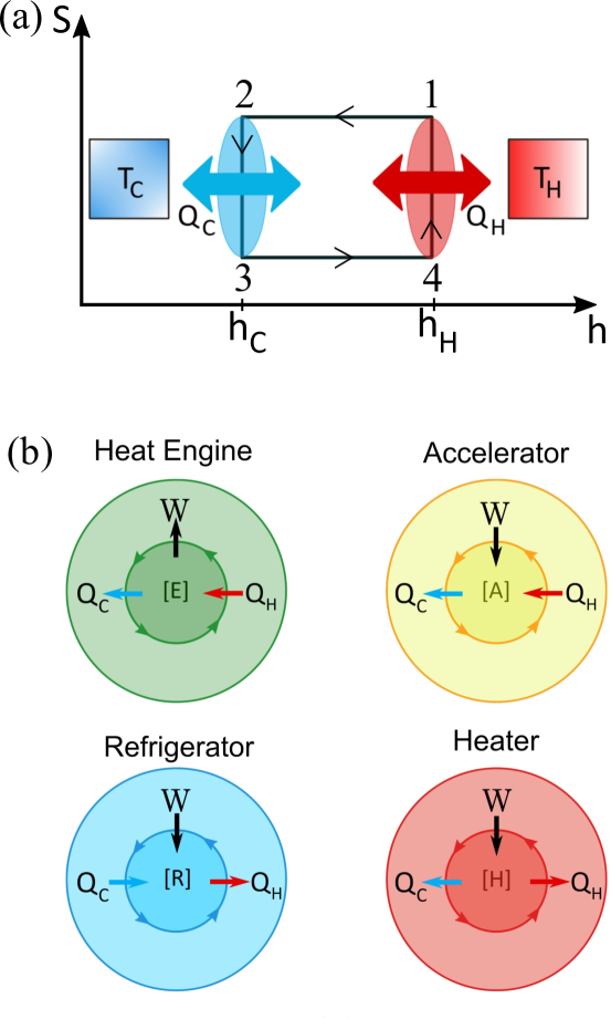
-
•
Engine [E]: Utilises the thermodynamic flow of heat to do work; .
-
•
Accelerator [A]: Increases the thermodynamic flow of heat using work; .
-
•
Refrigerator [R]: Utilises work to reverse the thermodynamic flow of heat; .
-
•
Heater [H]: Utilises work to transfer heat to both reservoirs; .
We use the convention that a negative value of heat or work is an output and a positive value an input. The thermodynamic flow of heat is a flow of heat from the hot to the cold reservoir.
In the thermodynamic limit the spacing between fermionic modes becomes infinitesimal, and summations over fermionic modes can be replaced by an integral . The total adiabatic work output for the cycle in Fig. 1 is then [22]
| (5) |
Here is the Fermi-Dirac distribution, which gives the occupation of the fermionic modes in thermal equilibrium.
II.3 Work and heat with an infinitesimal work step
In general, the thermal machine regime is determined by how energy levels respond to changes in and the number of energy levels contributing (i.e. temperature). To simplify our initial analysis, we consider an infinitesimal work stroke . For , Eq. (5) simplifies to
| (6) |
Here denotes an expectation value with respect to a thermal state at temperature . The quantity is the change in system energy due to the infinitesimal work stroke acting on a thermal state at temperature . Similarly, the heat associated with the hot and cold reservoirs are,
| (7) | ||||
For we have and and hence only accelerator or engine operation is possible, depending on the sign of work. We also have the relation:
| (8) |
where is the free energy of the system, with the partition function at temperature . Here the advantage of using an infinitesimal work stroke is clear, as it allows work and heat to be computed directly from the free energy. Using Eq. (2) the free energy is then [39]
| (9) |
Furthermore, using the partition function, we have
| (10) |
Here is the average transverse magnetization of the system (below we will also use the magnetization per particle ). Hence [22, 44]
| (11) |
i.e. the net work exchanged is directly proportional to the difference in transverse magnetization of the system at temperatures and .
Equation (11) takes an analogous form to the work output of an ideal gas Otto cycle, which for infinitesimal volume change is
| (12) |
with the pressure of the system. This pressure is monotonic with temperature, resulting in operation fixed by the sign of . Similarly, setting in Eq. (1) results in operation fixed by the sign of . In general, for simple non-interacting systems where all energy levels vary monotonically with the control parameter, the type of operation is fixed by the sign of the change in control parameter.
III Results
III.1 Thermal machine regimes for the transverse-field Ising model
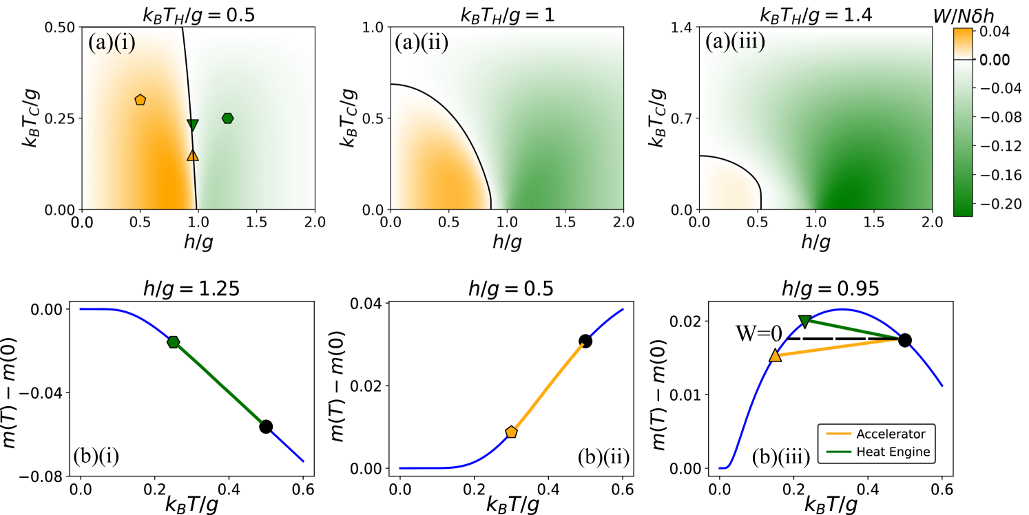
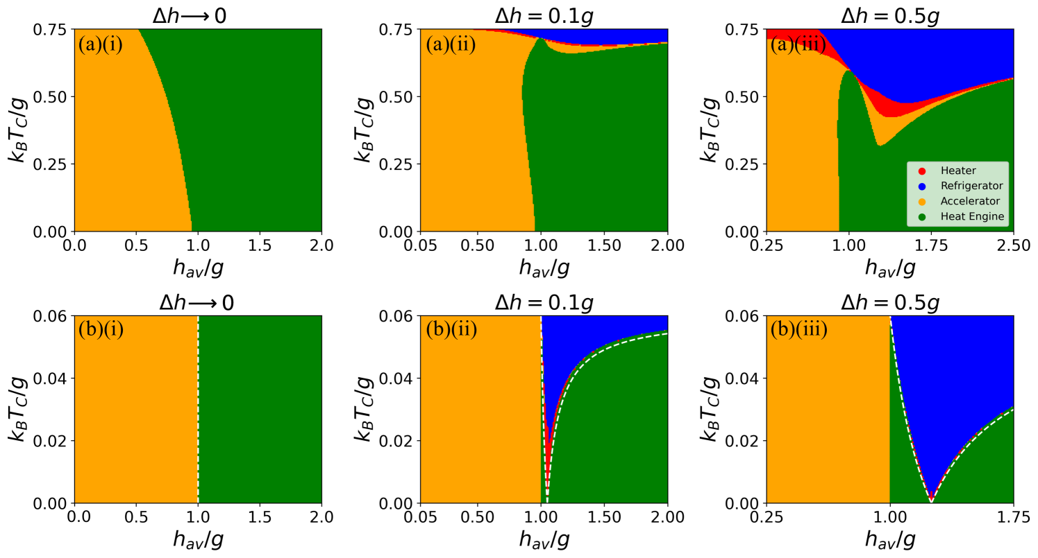
The work output and regimes of operation for the Otto cycle (Fig. 1) with infinitesimal work step are shown in Fig. 2(a). As already noted, with infinitesimal work step only accelerator or engine regimes are possible, with the regime of operation determined by the sign of (Eq. (11)). When the system operates as an engine, whereas for the system operates as an accelerator. For , the sign of work is reversed and the engine and accelerator regimes are switched.
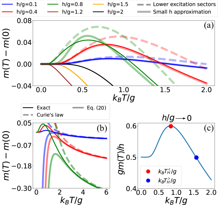
Due to the connection between work and , the regimes of operation can be understood from the behaviour of . Example behaviour of are illustrated in Fig. 2(b) and Fig. 3. The engine and accelerator regimes are separated by a boundary where and , which requires non-monotonic behaviour in , see Fig. 2(b)(iii).
III.1.1
For , the magnetization decreases monotonically as the temperature increases, see Fig. 2(b,i) and Fig. 3. Hence and the system operates as an engine. This can be understood as follows. The ground state for is paramagnetic and hence will have maximum transverse magnetization. Excited levels resulting from spin-flips [38, 45] will have small transverse magnetization, and hence as these become occupied ( is increased), will decrease. More precisely, using Eqs. (9), (10), we have
| (13) |
For we have for all .
III.1.2 and low temperature
For the system can operate as an engine or an accelerator dependent on and . For small and low temperatures we have and the system operates as an accelerator, see Fig. 2(b,ii) and Fig. 3. In this regime the free energy is,
| (14) |
where is obtained by expanding the spectrum Eq. (3) to linear order in . The net magnetization then satisfies
| (15) |
as anticipated.
This behaviour can be understood from domain-wall excitations above the ferromagnetic ground state. With periodic boundary conditions, these domain walls come in pairs [38] and the excitations take the form,
| (16) |
Here
| (17) |
is a product state with domain walls between spins , and , , where are the eigenstates of . The states Eq. (17) are degenerate for . The wavefunctions are obtained from perturbation theory in , which gives [38, 46, 47, 48]
| (18) |
with , . The superposition in Eq. (18) ensures , as the two domain walls cannot occur at the same location. To linear order in , the state Eq. (16) has energy and transverse magnetization . At low temperatures, increasing temperature results in increased occupation of the lower-energy domain-wall states (states with ), which increases the magnetization.
III.1.3 High temperature regime
For high temperatures, decreases monotonically with increasing temperature, see Fig. 3(a), and engine operation is observed, see Fig. 2(a). The high-temperature behaviour of can be obtained from Eq. (9) by expanding around , which gives
| (19) |
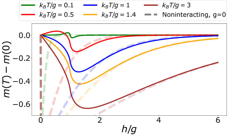
The dominant term in Eq. (19) follows Curie’s law and arises from high-temperature thermal fluctuations of the transverse spin. This results in engine operation and is present also in an ensemble of non-interacting spins. The effect of interactions on the magnetization appears at order and requires correlations between the axial and transverse spin directions (), which are suppressed at high temperatures. The result Eq. (19) predicts well the exact magnetization in the monotonic regime , see Fig. 3(b).
III.1.4 Intermediate temperature regime
A cross-over between the accelerator and engine regime requires non-monotonic and hence a peak where , see Fig. 2(b)(iii). This peak is only present for , see Fig. 3(a), and separates the low and high temperature regimes described above. The crossover ( line) can be determined by solving . To lowest order in we have
| (20) |
which is plotted in Fig. 3(c). From this plot it is clear that has a non-trivial solution only for . Here is the temperature the magnetization peaks, obtained from Eq. (20) by solving . The higher temperature is obtained from Eq. (20) by solving . For small the system operates strictly as an accelerator for and as an engine for .
With increasing , the boundary tends to move to lower , see Fig. 2(a). For , the point occurs at . A change in sign of requires a change in sign of within the range of thermally accessible . We have when
| (21) |
for some . From this we can estimate that the line occurs when , giving rise to a line that moves to lower as . Note the boundary requires using a spectrum beyond the perturbative approximation Eq. (15), which gives . Replacing by in Eq. (14) (equivalently expanding Eq. (9) in powers of ) gives
| (22) |
The approximation Eq. (22) qualitatively predicts the peak in magnetization for , see Fig. 3(a).
A more accurate expression for for can be obtained by expanding the full expression for to third order in . The resulting expression, however, is complicated,
| (23) |
with . The approximation Eq. (23) agrees well with the exact magnetization for , see Fig. 3(a).
III.1.5 Finite-size effects
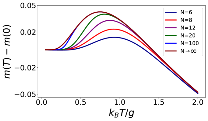
The free energy for the transverse field Ising model can also be calculated for a finite number of spins after accounting for parity [49, 50]. The magnetization for systems with a finite number of spins and are compared with the thermodynamic limit in Fig. 4. For the magnetization per particle agrees well with the thermodynamic limit. For smaller the magnetization is qualitatively similar to the thermodynamic limit, and results in strictly accelerator operation for sufficiently low temperatures of the hot bath and engine operation for sufficiently high temperatures [c.f. Fig. 3(c)]. We find decreases with decreasing ; hence the temperature range separating the strictly engine and accelerator regimes narrows as the system size is reduced, see Fig. 4. The decrease in with occurs because the sparsely spaced energy levels in finite-size systems require a higher temperature to obtain a given transverse magnetization. We observe a cross-over to monotonically decreasing for , as for the thermodynamic limit, with the precise cross-over sensitive to . As increases further the effect of interactions decreases and the finite-size results for converge to the thermodynamic limit even for small .
III.2 Magnitude of work output
We now briefly discuss the magnitude of work extracted (engine) or consumed (accelerator). In the high-temperature, low- limit, increases with increasing , see Fig. 2. This can be seen directly from the high temperature expansion Eq. (19), which also results in decreasing with increasing for fixed . In contrast, in the low-temperature, high- limit, decreases with increasing , see Fig. 2. When , the transverse magnetization can be approximated by the magnetization of non-interacting spins,
| (24) |
For low temperatures this gives , in which case we find increases with increasing for fixed . Both of these arguments also hold in the absence of interactions.
For , is largest around , see Fig. 5. This results in a peak in for , see Fig. 2. Such a peak has been discussed already in the low-temperature regime, in which case it can be explained in terms of a decreasing energy gap between the ground and first excited state [16]. At low temperatures and for , this results in a performance that exceeds that of non-interacting spins [16].
III.3 Finite-size work strokes
For an infinitesimal work stroke, the sign of the heat flows are fixed, restricting operation to either engine or accelerator, see Eq. (7). A finite-sized work stroke permits the thermal machine to operate as a refrigerator or a heater, see Fig. 6, where we have defined .
To see how refrigeration operation may appear, it is simplest to first consider very low temperatures, in which case only the ground and first excited states have any significant thermal occupation [16]. The analysis then proceeds as for a single spin-1/2 system [43]. For low temperatures the heat flows are,
| (25) | ||||
with the energy of the first excited level, which is the fermionic mode. From examination of Eq. (25), it is clear that low-temperature refrigeration (, ) occurs when
| (26) |
For Eq. (26) is satisfied when
| (27) |
The bounds of the inequality (27) accurately predict the low-temperature refrigerator boundary, see Fig. 6(b). Similar inequalities can be obtained from Eq. (26) for .
For higher temperatures, the analysis is qualitatively similar but complicated by the many levels present in the problem. This case has been discussed in recent works [37, 34, 22]. Notably, refrigerator operation is more effective when the temperature difference between and is small, and the influence of the critical point results in a peak in cooling capability [37]. Additionally, it was shown that as the size of the work stroke increases, the boundary of the refrigerator region expands to smaller [34]. This expansion of the refrigerator region becomes more pronounced with work strokes across the critical point, as seen in Fig. 6.
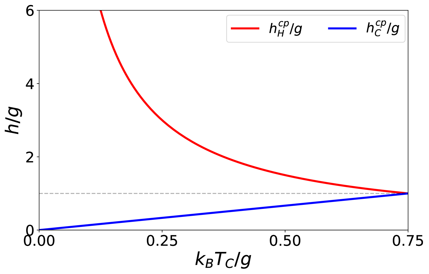
All four regimes of operation appear for finite at sufficiently high temperature, see Fig. 6(a). This gives rise to a “Carnot point” where and all four regimes intersect [43, 22]. A sufficient condition for is for all [22]. The ratio is insensitive to when , which gives [using Eq. (3)]. Substituting this into and setting gives values and where for given , and [22],
| (28) |
The field strengths and are shown in Fig. 7. The Carnot point appears when crosses , since . This is reasonable because the sign of is most sensitive to near , so small variations in can lead to changes in the sign of and . For small , the Carnot point will appear when , as then only a small is needed to change the flow of heat, see Fig. 6(a)(ii). As increases (), the accelerator and heater regimes shrink, and the system behavior converges to that of a noninteracting spin chain, where only the engine and refrigerator regimes remain.
When the sign of the heat flows are fixed and only accelerator or engine operation is possible. Furthermore, the boundary separating these two regimes is unaffected by at low temperatures, see Fig. 6. Focusing on just the ground and first excited state, as in Eq. (25), zero work output will occur when , in which case the work stroke causes no net change in the energy of the first excited state. This gives irrespective of .
IV Conclusion
We have presented the quantum thermal machine regimes for the transverse-field Ising model with an infinitesimal work stroke. In this scenario the heat flows are fixed by the temperatures of the hot and cold reservoirs. This results in either the heat engine or accelerator regime, dependent on the difference in equilibrium transverse magnetization at the two temperatures. We have identified the physical mechanisms behind the regimes of operation, connecting the low-temperature operation to the behavior of low-energy excitations and the high-temperature operation to an approximate equation of state for the system. This qualitative understanding also explains the regimes of operation for a finite-size work stroke when the difference in hot and cold reservoir temperatures are sufficiently large relative to the work stroke. Otherwise, refrigerator and heater regimes can emerge. Although most of our analysis here has been done in the thermodynamic limit, we have also shown that similar results hold in finite-size systems, as would be realised experimentally.
The realization of the transverse-field Ising model with either trapped ions or Rydberg atoms offers the potential to experimentally implement a many-body quantum thermal machine. Interactions between trapped ions are mediated by Coulomb forces, which can be modulated via optical dipole forces, and the transverse drive is an external magnetic field. Van der Waals forces mediate interactions between Rydberg atoms, and the transverse drive is a coherent laser. In both setups the work step can easily be implemented by varying the intensity of the transverse drive. Controlled heating and cooling of the system poses a challenge, but may be possible by applying external noise or light beams [51, 52]. The work done by the spins changes the power of the transverse drive, but the change is too small to be experimentally detectable 111To see this, first note that adiabatic engine operation requires a cycle time and therefore the change in power of the drive is . For a system driven by a magnetic field we have , with the magnetic dipole moment of the spins, while for a system driven by an electric field we have , with the electric dipole moment. Estimating and , with the Bohr magneton, the Bohr radius and the electron charge, gives for a magnetic drive and for an electrical drive, with the fine structure constant, being the area of the drive and . For an electric drive with a micron scale beam waist we have ; for a magnetic drive the output is even smaller.. The work done by the spins could instead by inferred from measuring the change in energy of the working substance itself [54] using site-resolved imaging [31, 55].
Our methodology and analysis will be useful in exploring other complex many-body quantum thermal machines, such as spin chains with long-range interactions and interacting Bose gases [7]. Diabatic work steps will likely modify the regimes of operation [43]. Considering infinitesimal work strokes would make diabatic operation amenable to a perturbative analysis [56] and allow counterdiabatic protocols to be incorporated [57], providing an interesting avenue for future research.
Acknowledgements.
This research was supported by The University of Queensland–IITD Academy of Research (UQIDAR), the Australian Research Council Centre of Excellence for Engineered Quantum Systems (CE170100009), and the Australian federal government Department of Industry, Science, and Resources via the Australia-India Strategic Research Fund (AIRXIV000025). We also acknowledge the support from the Indian Institute of Technology Delhi and SERB-DST, India.References
- Millen and Xuereb [2016] J. Millen and A. Xuereb, Perspective on quantum thermodynamics, New J. Phys. 18, 011002 (2016).
- Scovil and Schulz-DuBois [1959] H. E. D. Scovil and E. O. Schulz-DuBois, Three-level masers as heat engines, Phys. Rev. Lett. 2, 262 (1959).
- Geva and Kosloff [1992] E. Geva and R. Kosloff, A quantum-mechanical heat engine operating in finite time. A model consisting of spin-1/2 systems as the working fluid, J. Chem. Phys. 96, 3054 (1992).
- Peterson et al. [2019] J. P. S. Peterson, T. B. Batalhão, M. Herrera, A. M. Souza, R. S. Sarthour, I. S. Oliveira, and R. M. Serra, Experimental characterization of a spin quantum heat engine, Phys. Rev. Lett. 123, 240601 (2019).
- Niedenzu and Kurizki [2018] W. Niedenzu and G. Kurizki, Cooperative many-body enhancement of quantum thermal machine power, New J. Phys. 20, 113038 (2018).
- Mukherjee and Divakaran [2021] V. Mukherjee and U. Divakaran, Many-body quantum thermal machines, J. Phys.: Condens. Matter 33, 454001 (2021).
- Cangemi et al. [2024] L. M. Cangemi, C. Bhadra, and A. Levy, Quantum engines and refrigerators, Phys. Rep. 1087, 1 (2024), quantum engines and refrigerators.
- Dillenschneider and Lutz [2009] R. Dillenschneider and E. Lutz, Energetics of quantum correlations, EPL 88, 50003 (2009).
- Abah and Lutz [2014] O. Abah and E. Lutz, Efficiency of heat engines coupled to nonequilibrium reservoirs, EPL 106, 20001 (2014).
- Williamson et al. [2024] L. A. Williamson, F. Cerisola, J. Anders, and M. J. Davis, Extracting work from coherence in a two-mode bose–einstein condensate, Quantum Sci. Technol. 10, 015040 (2024).
- Bengtsson et al. [2018] J. Bengtsson, M. N. Tengstrand, A. Wacker, P. Samuelsson, M. Ueda, H. Linke, and S. M. Reimann, Quantum Szilard engine with attractively interacting bosons, Phys. Rev. Lett. 120, 100601 (2018).
- Chen et al. [2019] Y.-Y. Chen, G. Watanabe, Y.-C. Yu, X.-W. Guan, and A. del Campo, An interaction-driven many-particle quantum heat engine and its universal behavior, npj Quantum Inf. 5, 88 (2019).
- Carollo et al. [2020] F. Carollo, F. M. Gambetta, K. Brandner, J. P. Garrahan, and I. Lesanovsky, Nonequilibrium quantum many-body Rydberg atom engine, Phys. Rev. Lett. 124, 170602 (2020).
- Fogarty and Busch [2020] T. Fogarty and T. Busch, A many-body heat engine at criticality, Quantum Sci. Technol. 6, 015003 (2020).
- Boubakour et al. [2023] M. Boubakour, T. Fogarty, and T. Busch, Interaction-enhanced quantum heat engine, Phys. Rev. Res. 5, 013088 (2023).
- Williamson and Davis [2024] L. A. Williamson and M. J. Davis, Many-body enhancement in a spin-chain quantum heat engine, Phys. Rev. B 109, 024310 (2024).
- Estrada et al. [2024] J. A. Estrada, F. Mayo, A. J. Roncaglia, and P. D. Mininni, Quantum engines with interacting Bose-Einstein condensates, Phys. Rev. A 109, 012202 (2024).
- Watson and Kheruntsyan [2024] R. S. Watson and K. V. Kheruntsyan, Quantum many-body thermal machines enabled by atom-atom correlations, arXiv:2308.05266v3 (2024).
- Nautiyal et al. [2024] V. V. Nautiyal, R. S. Watson, and K. V. Kheruntsyan, A finite-time quantum Otto engine with tunnel coupled one-dimensional Bose gases, New J. Phys. 26, 063033 (2024).
- Nautiyal [2025] V. V. Nautiyal, Out-of-equilibrium quantum thermochemical engine with one-dimensional bose gas, arXiv:2411.13041 (2025).
- Yunger Halpern et al. [2019] N. Yunger Halpern, C. D. White, S. Gopalakrishnan, and G. Refael, Quantum engine based on many-body localization, Phys. Rev. B 99, 024203 (2019).
- Arezzo et al. [2024] V. R. Arezzo, D. Rossini, and G. Piccitto, Many-body quantum heat engines based on free fermion systems, Phys. Rev. B 109, 224309 (2024).
- Talkner et al. [2007] P. Talkner, E. Lutz, and P. Hänggi, Fluctuation theorems: Work is not an observable, Phys. Rev. E 75, 050102 (2007).
- Quan et al. [2007] H. T. Quan, Y.-x. Liu, C. P. Sun, and F. Nori, Quantum thermodynamic cycles and quantum heat engines, Phys. Rev. E 76, 031105 (2007).
- Plastina et al. [2014] F. Plastina, A. Alecce, T. J. G. Apollaro, G. Falcone, G. Francica, F. Galve, N. Lo Gullo, and R. Zambrini, Irreversible work and inner friction in quantum thermodynamic processes, Phys. Rev. Lett. 113, 260601 (2014).
- Porras and Cirac [2004] D. Porras and J. I. Cirac, Effective quantum spin systems with trapped ions, Phys. Rev. Lett. 92, 207901 (2004).
- Britton et al. [2012] J. W. Britton, B. C. Sawyer, A. C. Keith, C.-C. J. Wang, J. K. Freericks, H. Uys, M. J. Biercuk, and J. J. Bollinger, Engineered two-dimensional Ising interactions in a trapped-ion quantum simulator with hundreds of spins, Nature 484, 489 (2012).
- Bohnet et al. [2016] J. G. Bohnet, B. C. Sawyer, J. W. Britton, M. L. Wall, A. M. Rey, M. Foss-Feig, and J. J. Bollinger, Quantum spin dynamics and entanglement generation with hundreds of trapped ions, Science 352, 1297 (2016).
- Zhang et al. [2017] J. Zhang, G. Pagano, P. W. Hess, A. Kyprianidis, P. Becker, H. Kaplan, A. V. Gorshkov, Z.-X. Gong, and C. Monroe, Observation of a many-body dynamical phase transition with a 53-qubit quantum simulator, Nature 551, 601 (2017).
- Monroe et al. [2021] C. Monroe, W. C. Campbell, L.-M. Duan, Z.-X. Gong, A. V. Gorshkov, P. W. Hess, R. Islam, K. Kim, N. M. Linke, G. Pagano, P. Richerme, C. Senko, and N. Y. Yao, Programmable quantum simulations of spin systems with trapped ions, Rev. Mod. Phys. 93, 025001 (2021).
- Labuhn et al. [2016] H. Labuhn, D. Barredo, S. Ravets, S. de Léséleuc, T. Macrì, T. Lahaye, and A. Browaeys, Tunable two-dimensional arrays of single Rydberg atoms for realizing quantum Ising models, Nature 534, 667 (2016).
- Browaeys and Lahaye [2020] A. Browaeys and T. Lahaye, Many-body physics with individually controlled rydberg atoms, Nat. Phys. 16, 132 (2020).
- Kloc et al. [2019] M. Kloc, P. Cejnar, and G. Schaller, Collective performance of a finite-time quantum otto cycle, Phys. Rev. E 100, 042126 (2019).
- Piccitto et al. [2022] G. Piccitto, M. Campisi, and D. Rossini, The Ising critical quantum Otto engine, New J. Phys. 24, 103023 (2022).
- B. S et al. [2020] R. B. S, V. Mukherjee, U. Divakaran, and A. del Campo, Universal finite-time thermodynamics of many-body quantum machines from Kibble-Zurek scaling, Phys. Rev. Res. 2, 043247 (2020).
- Wang [2020] Q. Wang, Performance of quantum heat engines under the influence of long-range interactions, Phys. Rev. E 102, 012138 (2020).
- Solfanelli et al. [2023] A. Solfanelli, G. Giachetti, M. Campisi, S. Ruffo, and N. Defenu, Quantum heat engine with long-range advantages, New J. Phys. 25, 033030 (2023).
- Sachdev [2011] S. Sachdev, Quantum Phase Transitions, 2nd ed. (Cambridge University Press, 2011).
- Pfeuty [1970] P. Pfeuty, The one-dimensional Ising model with a transverse field, Ann. Phys. 57, 79 (1970).
- Alicki [1979] R. Alicki, The quantum open system as a model of the heat engine, J. Phys. A. 12, L103 (1979).
- Kosloff [1984] R. Kosloff, A quantum mechanical open system as a model of a heat engine, J. Chem. Phys. 80, 1625 (1984).
- Kosloff and Rezek [2017] R. Kosloff and Y. Rezek, The quantum harmonic Otto cycle, Entropy 19 (2017).
- Solfanelli et al. [2020] A. Solfanelli, M. Falsetti, and M. Campisi, Nonadiabatic single-qubit quantum Otto engine, Phys. Rev. B 101, 054513 (2020).
- Fusco et al. [2014] L. Fusco, S. Pigeon, T. J. G. Apollaro, A. Xuereb, L. Mazzola, M. Campisi, A. Ferraro, M. Paternostro, and G. De Chiara, Assessing the nonequilibrium thermodynamics in a quenched quantum many-body system via single projective measurements, Phys. Rev. X 4, 031029 (2014).
- Mbeng et al. [2024] G. B. Mbeng, A. Russomanno, and G. E. Santoro, The quantum Ising chain for beginners, SciPost Phys. Lect. Notes , 82 (2024).
- Subrahmanyam [2003] V. Subrahmanyam, Domain wall dynamics of the ising chain in a transverse field, Phys. Rev. B 68, 212407 (2003).
- Rutkevich [2010] S. B. Rutkevich, On the weak confinement of kinks in the one-dimensional quantum ferromagnet CoNb2O6, J. Stat. Mech.: Theory Exp. 2010 (07), P07015.
- Coldea et al. [2010] R. Coldea, D. A. Tennant, E. M. Wheeler, E. Wawrzynska, D. Prabhakaran, M. Telling, K. Habicht, P. Smeibidl, and K. Kiefer, Quantum criticality in an ising chain: Experimental evidence for emergent E8 symmetry, Science 327, 177 (2010).
- Katsura [1962] S. Katsura, Statistical mechanics of the anisotropic linear heisenberg model, Phys. Rev. 127, 1508 (1962).
- Białończyk et al. [2021] M. Białończyk, F. J. Gómez-Ruiz, and A. del Campo, Exact thermal properties of free-fermionic spin chains, SciPost Phys. 11, 013 (2021).
- Roßnagel et al. [2016] J. Roßnagel, S. T. Dawkins, K. N. Tolazzi, O. Abah, E. Lutz, F. Schmidt-Kaler, and K. Singer, A single-atom heat engine, Science 352, 325 (2016).
- Zou et al. [2017] Y. Zou, Y. Jiang, Y. Mei, X. Guo, and S. Du, Quantum heat engine using electromagnetically induced transparency, Phys. Rev. Lett. 119, 050602 (2017).
- Note [1] To see this, first note that adiabatic engine operation requires a cycle time and therefore the change in power of the drive is . For a system driven by a magnetic field we have , with the magnetic dipole moment of the spins, while for a system driven by an electric field we have , with the electric dipole moment. Estimating and , with the Bohr magneton, the Bohr radius and the electron charge, gives for a magnetic drive and for an electrical drive, with the fine structure constant and the area of the drive. For an electric drive with a micron scale beam waist we have ; for a magnetic drive the output is even smaller.
- Onishchenko et al. [2024] O. Onishchenko, G. Guarnieri, P. Rosillo-Rodes, D. Pijn, J. Hilder, U. G. Poschinger, M. Perarnau-Llobet, J. Eisert, and F. Schmidt-Kaler, Probing coherent quantum thermodynamics using a trapped ion, Nat. Commun. 15, 6974 (2024).
- Islam et al. [2011] R. Islam, E. E. Edwards, K. Kim, S. Korenblit, C. Noh, H. Carmichael, G.-D. Lin, L.-M. Duan, C.-C. Joseph Wang, J. K. Freericks, and C. Monroe, Onset of a quantum phase transition with a trapped ion quantum simulator, Nat. Commun. 2, 377 (2011).
- Scandi et al. [2020] M. Scandi, H. J. D. Miller, J. Anders, and M. Perarnau-Llobet, Quantum work statistics close to equilibrium, Phys. Rev. Res. 2, 023377 (2020).
- del Campo [2013] A. del Campo, Shortcuts to adiabaticity by counterdiabatic driving, Phys. Rev. Lett. 111, 100502 (2013).