Quasi-conjugate Bayes estimates for GPD parameters and application to heavy tails modelling

According to Damsleth (1975), the description of the conjugate class for gamma distributions relies on the so-called type II Gamcon distributions: for $x>0$, the density of the Gamcon II($c,\,d$) distribution with parameters $c>1$ and $d>0$ is

where $I_{c,\,d}=\int_{0}^{\infty}\Gamma(dx\,+\,1)(\Gamma(x))^{-d}(c\,d)^{-dx}\,dx$. Let in the following ${\mathbf{z}}$ $=$ $(z_{1},\dots,z_{k})$ denote a $k$-sample of realizations of i.i.d. random variables $Z_{1},\dots,Z_{k}$ issued from Gamma$(\alpha,\,\beta)$. According to Damsleth (1975), Theorem 2, the conjugate prior density on $(\alpha,\,\beta)$ with hyperparameters $\delta>0$ and $\eta>\mu>0$ is given by    $\pi_{\delta,\,\eta,\mu}(\alpha,\,\beta)\,=\,\pi(\alpha)\,\pi\left(\beta\left|\,\alpha\right.\right)\,$    where $\pi(\alpha)$ is the density of Gamcon II($c=\eta/\mu,\,d=\delta$) and $\pi(\beta|\,\alpha)$ is the density of Gamma($\delta\alpha\,+\,1,\,\delta\eta$). Then, the conditional density of $\alpha$ given ${\mathbf{z}}$, denoted $\,\pi(\alpha|\,{\mathbf{z}})$, is Gamcon II($\eta^{\prime}/\mu^{\prime},\,\delta^{\prime}$) with

and the conditional density of $\beta$ given $\alpha$ and ${\mathbf{z}}$, denoted $\pi(\beta|\,\alpha,\,{\mathbf{z}})$, is Gamma$(\delta^{\prime}\alpha\,+\,1,\,\delta^{\prime}\eta^{\prime})$. Remark 1 . – The hyperparameters $\eta$ and $\mu$ act on the sufficient statistics $s_{1}=\sum_{i=1}^{k}z_{i}$ and $s_{2}=\sum_{i=1}^{k}\ln{z_{i}}$, whereas $\delta$ tunes the importance of these modifications. When $\delta$ is a positive integer, the introduction of these prior distributions can loosely be interpreted as artificially adding $\delta$ observations with arithmetic mean $\eta$ in $s_{1}$ and another $\delta$ observations with geometric mean $\mu$ in $s_{2}$ with $\eta/\mu=c>1$. $\Box$

Our sampling scheme involves simulations from Gamcon II$(c,\,d)$ distributions with $c$ $=$ $c^{\prime}$ $=$ $\eta^{\prime}\big{/}\mu^{\prime}$, where $\eta^{\prime}$ and $\mu^{\prime}$ are given by (8), and moderate to large values of $d$ $=$ $d^{\prime}$ $=$ $\delta^{\prime}$ $=$ $\delta+k$. Up to our knowledge, there is no standard algorithm for simulating such distributions. The simulation method that we present is based on a normal approximation to Gamcon II distributions using Laplace’s method.

Gamcon II$(c,\,d)$ can be approximated by a normal distribution having the same mode. It is proved in Garrido (2002) that this mode, $M_{c,\,d}$, is the unique root of the equation

where $\psi$ denotes the digamma function: the derivative of the logarithm of $\Gamma(t)$. The standard deviation $S_{c,\,d}$ of the normal approximant distribution is computed through a Taylor expansion of the Gamcon II$(c,\,d)$ density in a neighborhood of its mode:

Garrido (2002) has established that $(1-1/d)/(\ln{c}+\ln{d/2})$ $\leq$ $M_{c,\,d}$ $\leq$ $2/\ln{c}$. In practice, $M_{c,\,d}$ is numerically approximated through the bisection method.

At each iteration, we simulate Gamcon II$(c^{\prime},\,d^{\prime})$ with the help of the independent Hastings-Metropolis algorithm, which requires a suitable proposal density. Actually, it is enough to make only one step of Hastings-Metropolis at each iteration of the Gibbs sampler: see Robert (1998). The proposal density must be as close as possible to the simulated density, Gamcon II$(c^{\prime},\,d^{\prime})$, and have heavier tails to ensure good mixing. Since Gamcon II densities have gamma-like tails, we cannot directly take the normal approximant density as a proposal. Rather, we have chosen a Cauchy proposal density as close as possible to the normal approximant density to Gamcon II$(c^{\prime},\,d^{\prime})$, i.e. with the same mode and modal value. Therefore at each iteration our Hastings-Metropolis step:

1. 1.

   independently simulates a new $Y$ from the Cauchy distribution with mode
   $M_{c^{\prime},\,d^{\prime}}$ and modal value $1\big{/}(S_{c^{\prime},\,d^{\prime}}\sqrt{2\pi})$ ;

2. 2.

   computes the ratio $\displaystyle{\rho\,=\,\min{\left[1,\,\frac{f^{\star}_{\mbox{\rm\scriptsize cauchy}}\left(\alpha^{(m)}\right)\,\xi_{c^{\prime},\,d^{\prime}}(Y)}{f^{\star}_{\mbox{\rm\scriptsize cauchy}}(Y)\;\xi_{c^{\prime},\,d^{\prime}}\left(\alpha^{(m)}\right)}\right]}\,,}$ where $f^{\star}_{\mbox{\rm\scriptsize cauchy}}$ denotes the density of $Y$ ;

3. 3.

   takes $\alpha^{(m+1)}$ $=$ $Y$ with probability $\rho$ and $\alpha^{(m+1)}$ $=$ $\alpha^{(m)}$ otherwise.

Since all the transition densities involved are positive, the resulting Markov chain $(\theta^{(m)})_{m\geq 0}$ is ergodic with unique invariant probability measure equal to the posterior distribution of $\theta$ given ${\mathbf{y}}$. Intensive numerical experiments reported in Garrido (2002) show that for $\delta>0.5$, this Gibbs sampler with one Hastings-Metropolis step at each iteration converges quickly to its invariant distribution. Actually, it seems that discarding the first $500$ iterations is sufficient. For $\delta\leq 0.5$, we observed numerical instabilities.

Bayesian inference on the GPD parameters $\alpha$, $\beta$ is based on the outputs of this algorithm when it has approximately reached its stationary regime. We then record a sufficient number of realizations $\alpha^{(m)}$ and $\beta^{(m)}$.

In this paper we suppose that no expert information is available for the choice of priors on the GPD parameters $(\alpha,\,\beta)$ and we thus take an empirical Bayes approach. Introduction of expert information is discussed in Appendix B.

We take $\delta=1$ both for convenience (for $\delta=1$, the prior $\pi(\alpha)$ reduces to a gamma distribution, see below) and because a small value of $\delta>0$ indicates little confidence in prior information (see Remark 1). Recall that we observed numerical instabilities of our Gibbs sampler for $\delta<0.5$. A natural approach to compute hyperparameter values of priors $\pi(\alpha)$ and $\pi(\beta|\,\alpha)$ is to equate some of their location parameters (e.g. the mean) to frequentist estimates of $\alpha$ and $\beta$, denoted here $\widehat{\alpha}$ and $\widehat{\beta}$. Recall that the mean of the prior distribution $\pi(\beta|\,\alpha)$ is $(\alpha+1)\big{/}\eta$. Taking this mean equal to $\widehat{\beta}=x_{n-k,\,n}$, the estimate induced by the Hill procedure, and replacing $\alpha$ by its Hill estimate yields $\eta=(\widehat{\alpha}\,+\,1)\big{/}\widehat{\beta}$. When $\delta=1$, the prior $\pi(\alpha)$ reduces to Gamma$(2,\,\ln{(\eta\big{/}\mu)})$. Its mean is $2\big{/}\ln{(\eta/\mu)}$. Solving the equation where this prior mean is set equal to $\widehat{\alpha}$ yields $\displaystyle{\mu\,=(\widehat{\alpha}+1)\;\left(\exp{\left(-\,2/\widehat{\alpha}\right)}\right)/\widehat{\beta}}.$

If prior modes are used instead of prior means, a similar approach leads to slightly different formulas for $\eta$ and $\mu$. Actually, with prior modes explicit expressions can be obtained for all $\delta>0$. However, preliminary numerical experiments yielded better estimates with prior means.

When the Gibbs sampler approximately reaches its stationary regime, $K$ values denoted $(\alpha^{(m)},\beta^{(m)})$, $m=1,\dots,K$, are saved. This sample is used to compute posterior means, medians or modes to estimate $(\alpha,\,\beta)$, leading to Bayesian estimates for $(\gamma,\,\sigma)$ and $q_{1-p}$. Remark 2 . – The posterior modes are more difficult to compute since one has first to construct smooth estimates of the joint posterior density of $\alpha$ and $\beta$. Numerical experiments reported in Garrido (2002) for both GPD generated data and excess samples led us to keep only posterior medians. $\Box$
Concerning the estimation of an extreme quantile $q_{1-p}$ (${\mathbf{y}}=(y_{1},\dots,y_{k})$ is a sample of excesses over a threshold $u$), a sample of values $\widehat{q}^{(m)}_{1-p}$ is computed using POT from the simulated $(\alpha^{(m)},\beta^{(m)})$’s:

Means, histograms and credibility intervals can then be computed and represented from (16). Bayesian credibility intervals for $\alpha$, $\beta$ and $q_{1-p}$ are obtained by sorting the corresponding simulated values obtained from the Gibbs sampler. See sections 3 and 4 below. The probability distribution of the observed sample ${\mathbf{y}}$ can be estimated either by GPD$(\widehat{\alpha},\,\widehat{\beta})$, or by the posterior predictive distribution. Similarly, predictive quantile functions can be approximated through

Three probability distributions in DA(Fréchet) were considered in order to produce various excess samples:

For each simulated data set and each value of $k$ $=$ $5,10,\dots,495$ Bayes-QC estimates of $\gamma$ and $q_{1-p}$, $\,p=1/5\,000$, are computed as the medians of the resulting $500$ $\,\widehat{\gamma}^{(m)}$’s and $\,\widehat{q}_{1-p}^{(m)}$’s given in the 500 last iterations of the Gibbs sampler. Figures 1–3 display the averages over the $100$ data sets of these Bayesian estimates of $\gamma$ and $q_{1-p}$ as functions of $k$. The means and modes were also computed and gave quite similar results. They are not displayed here. ML, MTI(DEdH) and ZipfG estimates of $\gamma$ and $q_{1-p}$, $\,p=1/5\,000$, were also computed for each of those simulated data sets and the same values of $k$. Figures 1–3 display the averages over the $100$ data sets of these estimates of $\gamma$ and $q_{1-p}$.

The left panels of Figures 1–3 show that our estimates of $\gamma$ based on posterior medians (continuous line curves) perform rather well compared to the other ones, and give estimates close to ML and ZipfG. The right panels of Figures 1–3 show that our estimates of $q_{1-p}$ are very close to those obtained by ML. Both give better estimates than MTI(DEdH) but in general do not perform as well as ZipfG, although they seem to be more stable as functions of $k$. Again, credibility intervals for $\gamma$ and $q_{1-p}$ and potential improvements when prior information is available are strong arguments supporting the use of our Bayesian procedure.

Monte Carlo simulations were also used to study whether Bayesian credibility intervals could be used as approximate frequentist confidence intervals for $\gamma$ and $q_{1-p}$. For each simulated data set, the last $500$ iterations of our Gibbs sampler provide $500$ estimates $\widehat{\gamma}^{(m)}$ and $500$ estimates $\widehat{q}_{1-p}^{(m)}$, $m$ $=$ $501,\dots,1\,000$. They can be sorted to provide approximate $90~\%$ credibility intervals for $\gamma$ and $q_{1-p}$. The precision of these credibility intervals was studied through Monte Carlo simulations: for each one of the three probability distributions considered and for each value of $k$, we counted the number of simulated data sets (out of $100$) for which the true values of $\gamma$ and $q_{1-p}$ fell within the corresponding $90~\%$ credibility intervals. Figure 4 exhibits the coverage rates for each simulated distribution and for $k=5,10,\dots,495$. These credibility intervals are very accurate for the Fréchet distribution. For the Log-Gamma distribution, the credibility intervals have good coverage rates for $q_{1-p}$ but not for $\gamma$.

This rather unexpected behavior when $\rho=0$ can be explained in terms of penultimate approximation, see Diebolt, Guillou and Worms (2003): it can be proved that for $\rho=0$, the distribution of excesses is better approximated by a GPD with scale parameter $\gamma+a_{k}(F)$, where $a_{k}(F)$ is some correction term, than by a GPD with scale parameter $\gamma$ (see, e.g., the paper coauthored by Kaufmann, pages 183–190 in Reiss and Thomas (2001) along with references therein and Worms (2001)). This explains why in the case $\rho=0$ the estimates of $\gamma$ strongly deviate from the true value. Furthermore, Diebolt et al. (2003) have established for all sufficiently regular estimators $(\widehat{\gamma},\,\widehat{\sigma})$ of the parameters $(\gamma,\,\sigma)$ such as ML or PWM, that when $\rho=0$ the estimated survival function $\bar{F}_{\widehat{\gamma},\,\widehat{\sigma}}$ is a bias-corrected estimate of $\bar{F}_{\gamma,\,\sigma}$. We think that this result partially explains the good and stable coverage rates observed for $q_{1-p}$ for the Log-Gamma distribution. These trials show that the credibility intervals computed through our procedure give very promising results.

For each one of the three simulated probability distributions and each value of $k\in\{5,10,\dots,495\}$ the 100 simulated data sets give 100 estimates of $(\gamma,q_{1-p})$. The empirical 0.05 and 0.95 quantiles of the previous estimates give $90\%$ Monte-Carlo Confidence intervals (MCCI) for $(\gamma,q_{1-p})$. The width of these MCCI’s are used in Figure 5 to compare the precision of our Bayes Quasi-conjugate $q_{1-p}$ estimator to ML, ZipfG and MTI(DEdH) estimators. For Burr data sets (left panel of Figure 5) ZipfG gives the most precise quantile estimators, it is followed by ML, Bayes-QC and MTI(DEdH). For Fréchet, Bayes-QC and ML have the best precisions. It is worth noting that the Bayes-QC is used here in its empirical version. Its precision will increase when combined with expert opinions.

In Figure 6 the average Bayes credibility intervals (averaged over the 100 simulated data sets) are compared to the $90\%$ Monte-Carlo Confidence intervals (MCCI) for our Bayes-QC estimator. For both Burr (left panel) and Fréchet (right panel) ditributions lower bounds of the average Bayes credibility intervals and MCCI are very close. Upper bounds of average Bayes credibility intervals are larger than those of MCCI. It is interesting to note that the width of the average Bayes credibility intervals are the narrowest for $k$ where Bayes estimate of $q_{1-p}$ is the closest to the true value $q_{1-p}$. This could be used to chose optimal values of the number of excesses $k$. Finally, Figure 1 suggests that the optimal value of $k$ in the Burr$(1,\,0.5,\,2)$ case is close to $90$. For $k=90$, the credibility intervals for both $\gamma$ and $q_{1-p}$ are still satisfactory.

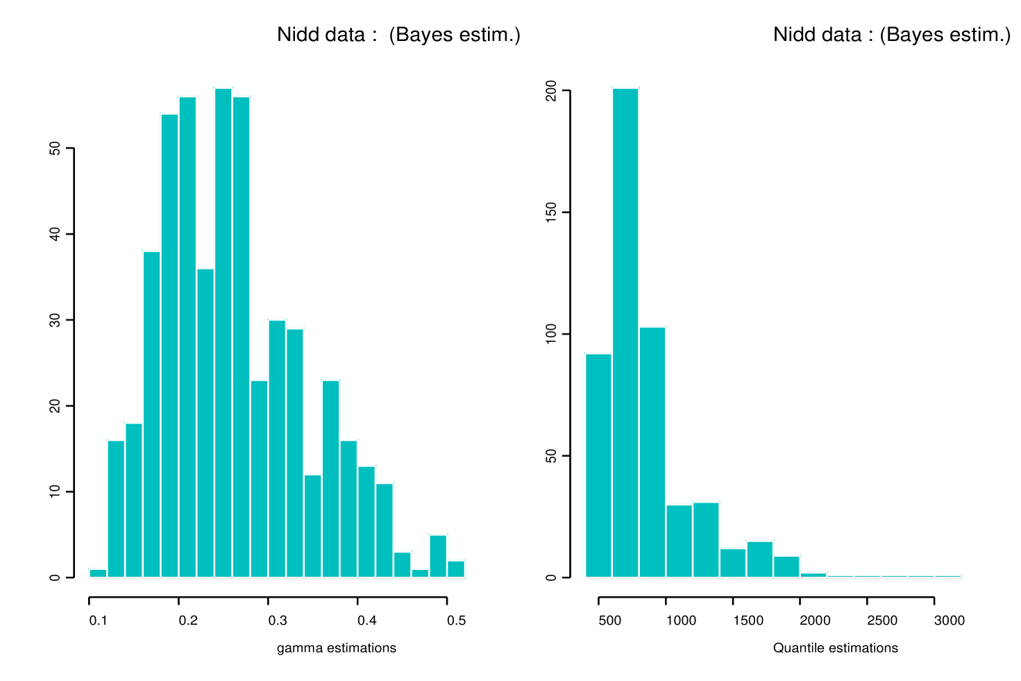
Bayes quasi-conjugate estimates and related $90~\%$ credibility intervals for $\gamma$ and $q_{1-p}$ are depicted in Figure 7 for several values of $k$. Compared to other estimators, our approach provides the most stable estimates as $k$ varies. For $8$ values of $k$ Grimshaw’s algorithm for computing ML estimates did not converge: see the broken ML curves in Figure 7. Histograms of $\gamma$’s and $q_{1-p}$’s for $k=82$ are displayed in Figure 8. Table 1 summarizes results of the estimation of the $50$-year and $100$-year return levels of the Nidd river when the threshold $u$ is set equal to either $100$ ($k=39$) or $120$ ($k=24$).

In the excess-of-loss (XL) reinsurance agreements, the re-insurer pays only for excesses over a high value $u$ of the individual claim sizes. The net premium is the expectation of the total claim amounts that the re-insurer will pay during the future period $[0,\,T]$: $\mathbb{E}(S_{N_{T}})$ $=$ $\sum_{i=1}^{N_{T}}Y_{i}$, where $N_{T}$ is the random number of claims exceeding $u$ during $[0,\,T]$ and $Y_{1},Y_{2},\dots$ are the amounts of excesses above $u$. If the $Y_{i}$’s are modeled by a GPD($\gamma$, $\sigma$) and the exceedance arrival process is modeled by a homogeneous Poisson process with annual rate $\lambda$, then the net premium over the coming year is approximated by $\mathbb{E}(S_{N_{1}})$ $\simeq$ $\mathbb{E}(N_{1})\,\mathbb{E}(Y_{i})$ $=$ $\lambda\sigma\big{/}(1-\gamma)$. Reiss and Thomas (1999, 2001) estimate the net premium of the Norwegian fire claims reinsurance by analysing a data set (see Table 2) of large Norwegian fire claims between 1983 and 1992 (1985 prices). They use a Bayesian inference method for the GPD parameters and assume that the exceedance process is Poisson. Independent gamma priors are used for $\lambda$ and $\alpha$ and an inverse-gamma prior, with parameters ($a$, $b$), is chosen for $\beta$. Posterior means of $\lambda$, $\alpha$ and $\beta$ are computed using Monte Carlo numerical approximations of integrals. Table 3 compares estimates of ($\gamma$, $\sigma$) and the net premium $\lambda\sigma\big{/}(1-\gamma)$ obtained by our quasi-conjugate approach with those obtained by Reiss and Thomas for ML and Bayesian estimates with different values of the hyperparameters $a$ and $b$ of the inverse-gamma. Our approach has the advantage of indicating the precision of the estimates.

References

- [1] Bacro, J., and Brito, M. Strong limiting behaviour of a simple tail Pareto-index estimator. Statist. Dec. 3, 133–143, (1993).
- [2] Balkema, A., and de Haan, L. Residual life time at a great age. Annals of Probability, 2, 792–804, (1974).
- [3] Beirlant, J., Dierckx, G., and Guillou, A. Estimation of the extreme value index and regression on generalized quantile plots. Preprint, Catholic University of Leuven, Catholic University of Leuven, Belgium. (2001).
- [4] Beirlant, J., and Teugels, J. Asymptotic normality of Hill’s estimator. In Extreme Value Theory (1989), eds., J. Hüsler and R.D. Reiss, Proceedings of the Oberwolfach Conference, 1987. Springer-Verlag New York.
- [5] Bottolo, L., Consonni, G., Dellaportas, P. and Lijoi, A. Bayesian analysis of extreme values by mixture modeling, Extremes 6, 25–47, (2003).
- [6] Breiman, L., Stone, C., and Kooperberg, C. Robust confidence bounds for extreme upper quantiles. J. Statist. Comput. Simul. 37, 127–149, (1990).
- [7] Caers, J., Beirlant, J., and Vynckier, P. Bootstrap confidence intervals for tail indices. Computational Statistics and Data Analysis 26, 259–277, (1998).
- [8] Castillo, E., and Hadi, A. Fitting the Generalized Pareto Distribution to data. J. Amer. Stat. Assoc. 92, 440, 1609–1620, (1997).
- [9] Coles, S. An introduction to statistical modelling of extreme values. Springer series in Statistics, 2001.
- [10] Coles, S., and Powell, E. Bayesian methods in extreme value modelling: A review and new developments. International Statistical Review 64, 1, 119–136, (1996).
- [11] Coles, S., and Tawn, J. A Bayesian analysis of extreme rainfall data. Applied Statistics 45, 4, 463–478, (1996).
- [12] Damsleth, E. Conjugate classes of Gamma distributions. Scandinavian Journal of Statistics: Theory and Applications 2, 80–84, (1975).
- [13] Davison, A., and Smith, R. Models for exceedances over high thresholds. J. R. Statist. Soc. B 52, 3, 393–442, (1990).
- [14] Dekkers, A., Einmahl J.H.J., and de Haan, L. A moment estimator for the index of an extreme-value distribution. The Annals of Statistics 17, 4, 1833–1855, (1989).
- [15] Diebolt, J., Guillou, A., and Worms, R. Asymptotic behaviour of the probability-weighted moments and penultimate approximation. ESAIM: Probability and Statistics 7, 219–238, (2003).
- [16] Dupuis, D. Exceedances over high thresholds: A guide to threshold selection. Extremes 3, 1, 251–261, (1998).
- [17] Embrechts, P., Klüppelberg, C., and Mikosch, T. Modelling Extremal Events. Springer, 1997.
- [18] Garrido, M. Modélisation des évènements rares et estimation des quantiles extrêmes, Méthodes de sélection de modèles pour les queues de distribution. PhD thesis, Université Joseph Fourier de Grenoble (France), 2002.
- [19] Grimshaw, S. Computing maximum likelihood estimates for the Generalized Pareto Distribution. Technometrics 35, 2, May, 185–191, (1993).
- [20] Haeusler, E., and Teugels, J. On asymptotic normality of Hill’s estimator for the exponent of regular variation. The Annals of Statistics 13, 2, 743–756, (1985).
- [21] Hill, B. A simple general approach to inference about the tail of a distribution. The Annals of Statistics, 3, 5, 1163–1174, (1975).
- [22] Hosking, J., and Wallis, J. Parameter and quantile estimation for the Generalized Pareto Distribution. Technometrics 29, 3, August, 339–349, (1987).
- [23] Pickands, J. Statistical inference using extreme order statistics. The Annals of Statistics, 3, 119–131, (1975).
- [24] Reiss, R., and Thomas, M. A new class of Bayesian estimators in paretian excess-of-loss reinsurance. Astin Journal 29, 2, 339–349, (1999).
- [25] Reiss, R., and Thomas, M. Statistical Analysis of Extreme Values. Birkhauser Verlag, 2001.
- [26] Robert, C.P. Discretization and MCMC Convergence Assessment. Lecture Notes in Statistics 135, Springer Verlag, 1998.
- [27] Schnieper, R. Praktische Erfahrungen mit Grossschadenverteilungen. Mitteil. Schweiz. Verein Versicherungsmath, 149–165, (1993).
- [28] Schultze, J., and Steinebach, J. On least squares estimates of an exponential tail coefficient. Statist. Decisions 14, 353–372, (1996).
- [29] Singh, V., and Guo, H. Parameter estimation for 2-parameter Generalized Pareto Distribution by POME. Stochastic Hydrology and Hydraulics 11, 3, 211–227, (1997).
- [30] Smith, R. Estimating tails of probability distributions. The Annals of Statistics 15, 3, 1174–1207, (1987).
- [31] Smith, R., and Naylor, J. A comparison of maximum likelihood and Bayesian estimators for the three-parameter Weibull distribution. Appl. Statist. 36, 3, 358–369, (1987).
- [32] Tancredi, A., Anderson, C. and O’Hagan, A. A Bayesian model for threshold uncertainty in extreme value theory. Working paper 2002.12, Dipartimento di Scienze Statistiche, Universita di Padova. (2002).
- [33] Worms, R. Vitesse de convergence de l’approximation de Pareto Généralisée de la loi des excès. Comptes-Rendus de l’Académie des Sciences, série 1, Tome 333, 65–70, (2001).