Quasi-periodic dipping in the ultraluminous X-ray source,
NGC 247 ULX-1
Abstract
Most ultraluminous X-ray sources (ULXs) are believed to be stellar mass black holes or neutron stars accreting beyond the Eddington limit. Determining the nature of the compact object and the accretion mode from broadband spectroscopy is currently a challenge, but the observed timing properties provide insight into the compact object and details of the geometry and accretion processes. Here we report a timing analysis for an ks XMM-Newton campaign on the supersoft ultraluminous X-ray source, NGC 247 ULX-1. Deep and frequent dips occur in the X-ray light curve, with the amplitude increasing with increasing energy band. Power spectra and coherence analysis reveals the dipping preferentially occurs on ks and ks timescales. The dips can be caused by either the occultation of the central X-ray source by an optically thick structure, such as warping of the accretion disc, or from obscuration by a wind launched from the accretion disc, or both. This behaviour supports the idea that supersoft ULXs are viewed close to edge-on to the accretion disc.
keywords:
Accretion discs – X-rays: binaries – X-rays: individual: NGC 247 ULX-11 Introduction
Ultraluminous X-ray sources (ULXs) are X-ray bright, off-nuclear sources with luminosity (see Kaaret et al. 2017 for a review). Proposed explanations for these luminous sources include i. sub-Eddington accreting stellar mass compact objects whose radiation is beamed into our line of sight (King et al. 2001); ii. stellar-mass BHs in a super-Eddington regime (Poutanen et al. 2007) or, iii. intermediate-mass black holes accreting at sub-Eddington rates from low-mass companion stars (Colbert & Mushotzky 1999, Farrell et al. 2009).
The recent detection of coherent pulsations in several ULXs indicates they are powered by neutron stars (NS) accreting at very high Eddington rates, with luminosities up to (Bachetti et al. 2014, Israel et al. 2017a, b, Carpano et al. 2018; Sathyaprakash et al. 2019, Rodriguez Castillo et al. 2019, Chandra et al. 2020). Pulsations are not always detectable as high count rates and pulsed fraction are required. In the absence of pulsations, spectral analysis alone makes it difficult to distinguish between a BH or NS candidate (e.g. NGC 1313 X-1, Walton et al. 2020), which means that NSs are likely numerous among the compact objects of ULXs (King & Lasota 2019; Pintore et al. 2017; Walton et al. 2018; Middleton & King 2017; Wiktorowicz et al. 2019).
Fourier timing techniques are powerful tools for investigating in a model-independent way the geometry of accretion discs, the size scales involved, and the nature of the compact objects (e.g. Middleton et al. 2007; Heil et al. 2009; Pinto et al. 2017; Kara et al. 2020). For instance, the presence of time lags between certain energy bands identifies different regions of X-ray emission in the accretion disc. The soft time lags found in three ULXs indicates that substantial Compton down-scattering is occurring in the outer disk (e.g., De Marco et al. 2013; Pinto et al. 2017; Kara et al. 2020). Power spectral density (PSD) analysis allows us to distinguish different accretion processes occurring at various accretion rate and identify different zones within the accretion disc.
Dipping behaviour in the X-ray light curve have also been observed in some ULXs, e.g. NGC 55 (Stobbart et al. 2004), M 94 (Lin et al. 2013), NGC 628 (Liu et al. 2005), NGC 5408 X-1 (Pasham & Strohmayer 2013; Grisé et al. 2013 and M 51 ULX-7 (Hu et al. 2021; Vasilopoulos et al. 2021). The number of dips observed in these sources has so far been limited, however they suggest we are viewing these sources at high inclination or could be evidence for a precessing disc.
NGC 247 ULX-1 is a supersoft ultraluminous X-ray source. It is unique in that it switches between the soft ultraluminous X-ray state (SUL) and the supersoft ultraluminous state (ULS or SSUL, e.g. Feng et al. 2016). Two previous short ( ks), XMM-Newton observations revealed strong dips in source flux in the light curve. These dips lasted several ks with the flux decreasing by an order of magnitude (Feng et al. 2016). In this paper we report a timing study of the dipping in the light curves of NGC 247 ULX-1 using a recently awarded ks XMM-Newton campaign (PI: Pinto). PSD analysis reveals multiple preferred periodic-like timescales for the dips. A detailed spectral analysis is provided in two companion papers: Pinto et al. 2021 on the high-resolution spectroscopy and D’Aì et al. in prep on the broadband spectroscopy.
2 Observations and data analysis
NGC 247 ULX-1 was observed 8 times by XMM-Newton over 1 month, starting 2019-12-03 (see Pinto et al. 2021 for observation details). Seven observations have duration ks and one lasts for ks. Two short ( ks) observations from 2016 are not included in this analysis as they are too short to probe Fourier frequencies below Hz.
The EPIC-pn Observation Data Files (ODFs) were processed following standard procedures using the XMM-Newton Science Analysis System (SAS; v19.0.0), using the conditions PATTERN 0–4 and FLAG = 0. Source counts were extracted from a circular region with radius 20 arc seconds. The background is extracted from a large rectangular region on the same chip, avoiding the Cu ring on the outer parts of the chip. Following Alston et al. (2013, 2019) for flares with duration s, the source light curve was cut out and interpolated between the gap by adding Poisson noise using the mean of neighbouring points. The interpolation fraction was typically %. High background segments, typically towards the end of the revolutions (e.g. revolutions (revs) ), were excluded from the analysis.
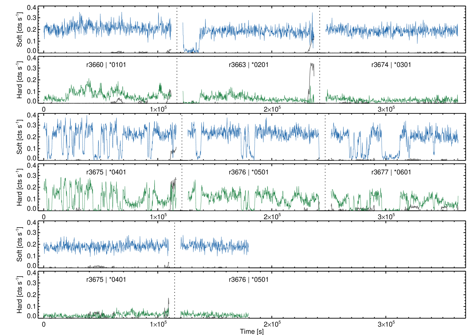
Figure 1 shows the background subtracted light curves for the keV (hereafter soft) and keV (hereafter hard) bands. These bands are motivated by broadband spectral analysis in Pinto et al. 2021 and D’Ai et al. in prep. Above keV the light curve is dominated by the background so we exclude it from the PSD analysis in Sec. 3.1, however these bands are used where appropriate in Sec. 3.6.
Clear dipping behaviour is apparent in four of the observations (revs ), with the dip duration ranging from ks. Four observations do not show any obvious dipping behaviour: revs . We therefore divide the observations into two data sets - the ‘dip’ and ‘non-dip’ segments. With the exception of rev , the dip segments have higher source flux and are spectrally harder (see also D’Ai et al. in prep, Pinto et al. 2021). In the following analysis, we use a segment length of ks for the dip epochs and ks for the no-dip epochs, owing to the shorter duration of rev .
3 Timing analysis
3.1 The power spectrum
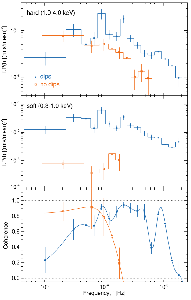
The PSD was estimated using the standard method of calculating the periodogram (e.g. Priestley 1981), with an normalisation, then averaging over segments at each Fourier frequency. Non-overlapping neighbouring frequency bins are then averaged (see e.g. Vaughan et al. 2003). In order to pick out features over a broad range of frequencies we used a geometrically averaged frequency bins, each bin spanning a factor in frequency larger than the previous bin. Figure 2 shows the soft and hard band noise-subtracted PSDs in units of for both the dipping and non-dipping segments (the noise is estimated from standard formulae, e.g. Vaughan et al. 2003).
The dipping observations show clear peaks in power at Hz and Hz. A further broader peak can be seen at Hz. At frequencies below Hz the PSD is rolling over towards zero power. With the exception of the appearance of narrow peaks in power, the shape of the dip and no-dipping segments in the hard band looks similar. The non-dip PSD has a smooth power-law like frequency dependence, with a steeper slope in the hard band.
3.2 Coherent variations
We study the correlated variations between the two bands using the Fourier coherence. This provides a measure of the linear correlation between two time series as a function of Fourier frequency, in the range [0,1] (Vaughan & Nowak 1997). We estimated cross-spectrum, , by first averaging the complex values over non-overlapping segments, then averaging over neighbouring frequency bins, in a similar manner to the PSD. This amplitude part of the cross-spectrum gives the coherence, , which is then corrected for Poisson noise, see e.g. Uttley et al. 2014 for more details.
The coherence is shown in Figure 2 for both the dipping and non-dipping light curves. A simple cubic spline has been fit to the data to illustrate the frequency dependence of the data. The coherence is high () at frequencies where the soft and hard band PSDs peak, and drops at frequencies between these peaks in power. In contrast, a high coherence at low frequencies is observed in the non-dipping light curves, which falls off sharply to zero at Hz, most likely caused by the onset of Poisson noise at high frequencies.
The phase part of the cross-spectrum provides an estimate of the frequency dependent delay between , which can be converted to a time delay in seconds (Vaughan & Nowak 1997). We estimated this for both the dipping and non-dipping segments and found the delay is consistent with zero lag at all Fourier frequencies.
3.3 Modelling the power spectra
To characterise the observed peaks in variability power in the dip segments we modelled the PSD using multiple Lorentzian functions;
| (1) |
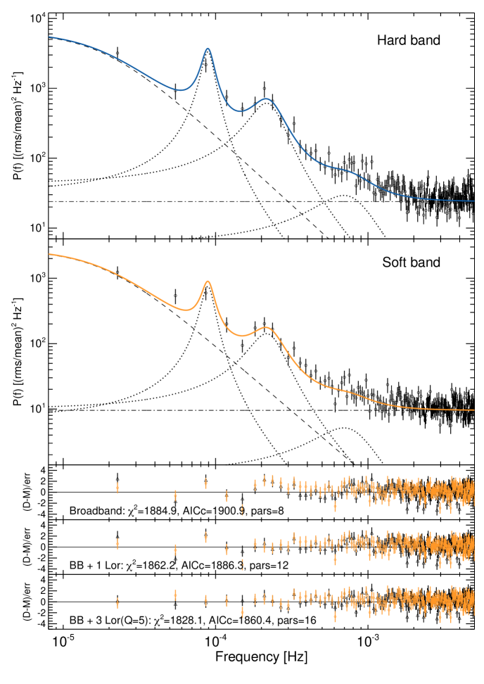
where and are the line centroid and width parameters, respectively, and is a normalisation. The quantity gives a measure of how narrow, or ‘coherent’ the Lorentzian is. Here, instead of subtracting the Poisson (‘white’) noise in each PSD band we model this with an additive constant, . The hard and soft band have similar shape, so we jointly model the data, allowing certain parameters untied in model variants described below. The models are fit by minimising the statistic within the package xspec. The parameter and space were explored with Goodman & Weare (2010) Markov Chain Monte Carlo (MCMC) sampling. Quoted parameter errors are from the credible intervals. We used a linear binning factor of to improve the frequency resolution in the modelling. With a time bin s this results in a combined total of data bins for the soft and hard PSDs. The resulting PSDs and model fits along with the model standard residuals are shown in Figure 3.
The Akaike information criterion was used for model selection to compare models with additional complexity (Akaike 1974). The corrected form of this statistic takes account for the bias from the small sample size, which can be expressed as
| (2) |
where is the number of free model parameters, is the number of data bins in the PSD and is used to represent the negative of twice the logarithm of the likelihood of the model. The model with the lowest is the most preferred over all models. The , with a suggesting weak evidence in favour of the model. A suggests moderate evidence for the model and implies the model is strongly favoured (e.g. Burnham & Anderson 2007).
We initially model the PSDs using a single broad Lorentzian component (model: Broadband), with all parameters free, giving /dof (degrees of freedom) . The and AICc are given in Table 1 and the residuals of this model are shown in Figure 3. The next more complex model has the addition of a narrower Lorentzian () at Hz (model: BB+1Lor). With and tied between the two PSDs and and free, this improves the fit by for 4 additional dof. Compared to the ‘Broadband’ model the , indicating a strong preference for the more complex model. Allowing any of the parameters to be untied between the two PSDs does not notably improve the model fit.
The addition of a Lorentzian () with Hz (model BB+2Lor) reduces the for 4 additional dof. Untying the parameters of the additional Lorentzian between the two PSDs does not significantly improve the fit. Compared to the previous model the , again suggesting the more complex model is strongly supported.
The most complex model we test involves the addition of a narrow Lorentzian () with Hz (model: BB+3Lor). With all but the normalisation parameters tied across the two energy bands, the best fit model gives /dof , with 4 additional parameters compared to the previous model. The , again suggesting the more complex model is strongly supported. The low sampling resolution at low frequencies means the fit is largely insensitive to of the broadband Lorentzian, so we fix this to zero (model: BB+3Lor()). This gives no notable change to the fit, but helps remove some parameter degeneracies between and . Equally, and (i.e. the Lorentzian at Hz also display degeneracies, so we fix these at approximately the median MCMC values of (model: BB+3Lor()). The parameters for this model are shown in Table 2. The addition of more Lorentzian components provides an improvement of , so we do not consider those models further.
For the no-dip segments, a single zero-centered Lorentzian provides an adequate description of the hard band PSD. The additional parameters are Hz and . Additional components do not significantly improve the AICc so we do not explore this further.
| Model | / d.o.f | |||
|---|---|---|---|---|
| Broadband (BB) | 8 | 1884.9 / 1594 | 1900.9 | 40.5 |
| BB+1Lor | 12 | 1862.2 / 1590 | 1886.3 | 25.9 |
| BB+2Lor | 14 | 1847.2 / 1588 | 1875.5 | 15.1 |
| BB+3Lor | 18 | 1824.1 / 1584 | 1860.5 | 0.1 |
| BB+3Lor () | 17 | 1826.4 / 1585 | 1860.8 | 0.4 |
| BB+3Lor () | 16 | 1828.0 / 1586 | 1860.4 | *min* |
| Comp. | Q | ||||
|---|---|---|---|---|---|
| - | |||||
| fixed | - | ||||
| 5f | |||||
| 2 | |||||
| 1 |
3.4 Periodogram of dipping observations
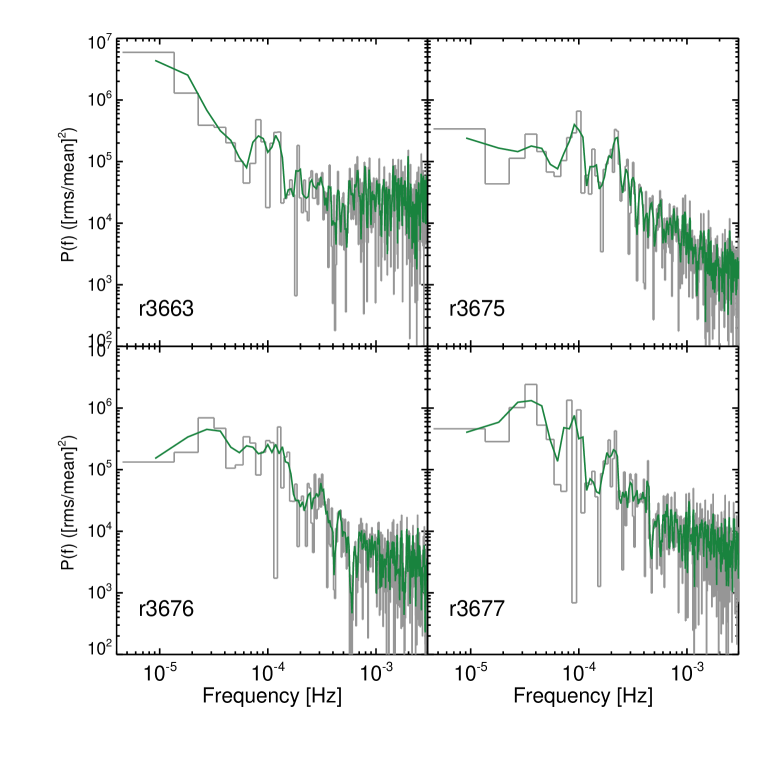
To check that no one particular observation is driving the peaks in the average PSD we estimate the unbinned periodogram. Figure 4 shows the periodogram for the four dipping observations. It is well known that the periodogram estimate at each frequency follows a distribution so large scatter around the true underlying power spectrum is expected (e.g. Priestley 1981). We therefore also show a Gaussian smoothed with periodogram over neighbouring frequency bins. Peaks in power at Hz and Hz are found in each periodogram. Another peak or bend can be seen at Hz in all but rev , which shows power at lower frequencies.
We refit these periodograms using the maximum likelihood methods (MLE) for unbinned periodograms outlined in Vaughan (2010) and Barret & Vaughan (2012). The power spectral modelling results are consistent with those found in Section 3.3, so we do not show those here. For rev the Lorenztzian centroids and appear to shift to higher frequencies, however modelling reveals these to be consistent within error bars with the other revs. The only notable difference is the increase in power at low frequencies in rev , which requires a zero-centered Lorentzian with width Hz. Removing rev from the combined PSD modelling in Section 3.3 does not significantly alter the results, so we choose to leave it in to increase the number of estimates in each frequency bin.
3.5 Change point analysis
In order to study what aspect of the dips is causing the peaks in the power spectra, we modelled the abrupt light curve changes in the dip segments using change point analysis. The R package bcp111https://cran.r-project.org/web/packages/bcp/ was used which implements the Bayesian change point method of Wang & Emerson 2015. This partitions the light curve into constant mean ‘blocks’ between change points. MCMC sampling is used to model the posterior probability at each change point, , defined between [0,1]. Given the sharp changes in the light curves when dipping occurs, this method is particularly well suited to the data.
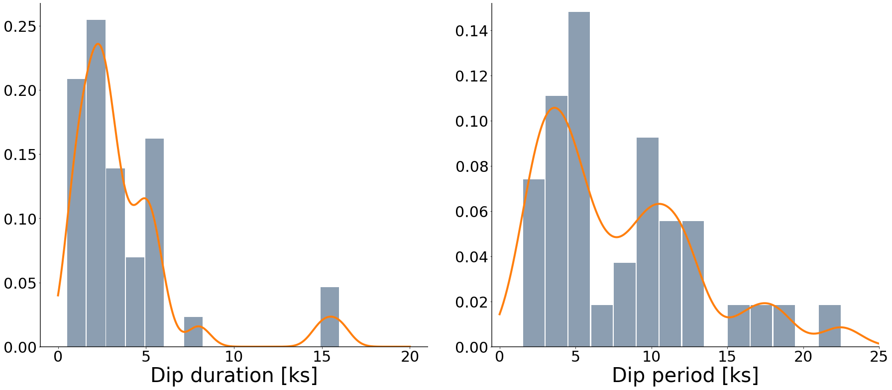
The Poisson noise starts to dominate at Hz so a time bin of s was used in order to smooth over any noise variations. A posterior probability was used to identify significant change point locations. From these we determine the dip onset time , dip duration , and dip midpoint, . The period is then taken as the time between successive dip midpoints.
Figure 5 shows the distribution of and for all four dipping observations. A Gaussian kernel density estimate is overlaid on the observed distributions. The distribution of peaks at ks and falls off approximately log-normally with increasing dip duration, i.e. there is a much larger probability for shorter dips. The distribution of is multi-modal with peaks at and ks, with a smaller probability of periods at ks. A similar distribution is observed if we represent the as the time between successive , suggesting no relationship between the duration of the dips and the dip period.
3.6 Variability spectra
We study the energy dependence of the variability at a given timescale using frequency resolved covariance spectra (Wilkinson & Uttley 2009). Using a high S/N reference band, the correlated variability is picked out in a given comparison band, thus improving the S/N of the variability spectrum compared to traditional rms spectra. We compute the covariance spectra in the Fourier domain (Uttley et al. 2011; Cassatella et al. 2012; Uttley et al. 2014). The keV band is used as the broad reference band, but the choice of this band does not affect the shape of the resultant covariance spectra.
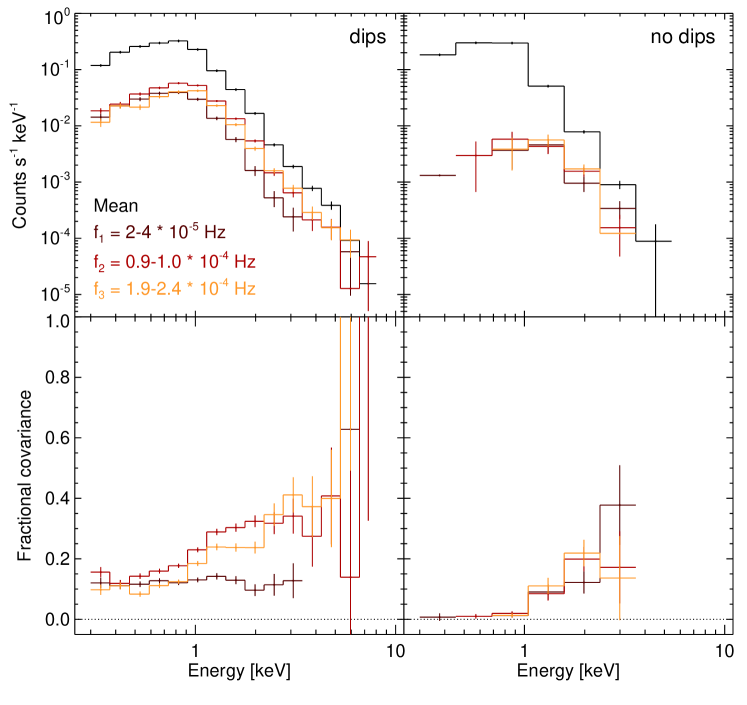
We estimate covariance spectra in three frequency bands: Hz, Hz and Hz. These timescales probe the long timescale spectral variability as well as the spectral variability associated with the two prominent dipping timescales. Figure 6 shows the resulting variability spectra. The top panels shows these data in absolute units () whilst the lower panels show the variability spectra in fractional () units. In the dipping segments, the long timescale spectral variability is approximately flat, with a rms amplitude. The dipping timescales, and , show an approximately linear dependence with energy, with larger variability amplitude at higher energies. This is true of all frequency bands up to higher frequencies, but we do not show those here.
For the dipping segments, as an additional check, we calculate the variability amplitude of each of the components in the preferred model (BB+3Lor ) by integrating the rms in each Lorentzian component. This shows the same trend in energy space as the frequency dependent covariance spectra. For the no-dip segments, the fractional variability amplitude is almost below keV, with a sharp increase in rms for energies above this.
4 Discussion
4.1 The dipping behaviour
The light curves of NGC 247 ULX-1 display deep and quasi-periodic dips imprinted on top of stochastic noise variations. Modelling the PSD with multiple Lorentzians reveals three preferred timescales for the dipping behavior. The peak in power of a Lorentzian occurs at frequency (see e.g. Belloni et al. 2002). For the preferred model, this gives Hz, Hz, Hz and Hz. The coherence between the hard and soft bands is high () at the Lorentzian peaks and drops where the Lorentzians overlap, providing further evidence for multiple dipping timescales.
Time series change point analysis reveals the dip periods, , cluster around and ks. This distribution of is consistent with the peak timescales observed in the power spectra (see Figure 3). The Lorentzian values tell us that there is some scatter around a preferred periodicity, as is observed in the change point period analysis. The dip durations preferentially take on values between ks, which will add some additional broadening to the measured Lorentzian values. There are several broad dips with ks, which clearly stand out from the other measured dip durations in Figure 5. This could be suggesting an alternative mechanism or timescale for these longer duration dips.
The change point analysis does not find any periods with s suggesting this analysis is either insensitive to this dips, e.g. they could be of lower amplitude and therefore harder to detect, in agreement with the lower amplitude of the Lorentzian . Alternatively, this high frequency component is related to an increase in the broadband noise continuum, which appears when the source enters the higher-flux / dipping epochs.
The time averaged and frequency resolved covariance spectra in Figure 6 show that the variations are larger at higher energies in both the dip and no-dip epochs. The exception being the Hz frequency band in the dip epochs. Here, the fractional covariance is independent of energy. The coherence between the soft and hard bands (see Figure 2) also drops to at these frequencies. This suggests that the long timescale variability is different to the dip generating mechanism at shorter timescales.
4.2 Origin of the dips in NGC 247 ULX-1
Assuming a black hole with , the peak timescales Hz correspond to an orbital radius () of cm, or (where ). A similar value is obtained for the case of a NS compact object. In both cases, this region is very distant from the compact object, suggesting an origin in the outer accretion flow. Two likely scenarios for the dips are warping of an accretion disc seen close to edge on, periodically obscuring the central source each orbit, or, the launching of a wind following changes in local . Alternatively, a combination of both processes could be causing the dips at different timescales.
The radius associated with Compton scattering through a medium around the spherisation radius can be expressed as (where is the speed of light, is the Thomson scattering cross-section, is the electron density, and is the timescale for photons to escape) would be of the order of cm, assuming a disc-like density ( cm-3), while such radius would be comparable ( cm) if we adopt a wind-like density ( cm-3). On the other hand, the wind radius, (where is the ionising luminosity and the ionisation parameter), that we estimate from the best-fit parameters of the XMM-Newton RGS-EPIC joint fit is also around cm (see Pinto et al. 2021). The lower density assumption is favoured as this agrees with both the outflow and dip timescale properties.
The mid plane of the accretion disc, i.e. the spherisation radius where the disc height is comparable to the distance from the accretor, is instead (assuming a standard and , which would be sufficient to achieve for ). This means that the timescales of the variability detected in NGC 247 ULX-1 are likely associated with the outer disc and, most likely, with the region where the wind becomes optically thin (e.g. cm-3) and rather than with the inner accretion flow or the optically thick wind ( cm-3) which would be expected near the spherisation radius. For a comparison, the wind photosphere in the Galactic super-Eddington source SS 433 is cm (see, e.g. Fabrika 2004), which further indicates that NGC 247 ULX-1 quasi-periodic dips might be associated with some structure present in the outer disc where the photosphere becomes optically thin.
The presence of dips and their long timescales argue in favour of a moderate-to-high inclination in this source, which agrees with the scenario in which soft ULXs are primarily seen along the edge of the wind. The dips seen in both BH and NS X-ray Binaries (XRBs) are believed to be caused by periodic obscuration of the central X-ray source by structure located in the outer regions of a disc. These dips are observed in sources at high inclination ( deg, e.g. Frank et al. 1987). For NGC 247 ULX-1, Yao & Feng (2019) derived an deg via modeling the UV/optical spectral energy distribution (SED) with an irradiation model, providing further evidence for a high inclination viewing angle in this source. Additionally, winds observed in BH or NS X-ray binaries (XRBs) have been mostly observed in sources in which the disc is inclined at a large angle to the line of sight (e.g. Ponti et al. 2012; Díaz Trigo & Boirin 2016).
Given the difficulty to access the inner regions of the accretion flow, mostly obscured by the scale height of the disc at the spherisation radius and the wind, we are not surprised that we did not detect the time lags between the soft and hard band that have been found in other, harder, ULXs. At these angles, the photons would undergo loads of Compton scattering, losing the original information.
If the dips are caused by a wind structure, what is not clear is whether the short-term variations in optical depth are just stochastic variability (at a given ) due to the clumpy nature of the wind. Alternatively, each variation corresponds to a change in the underlying variability in the local accretion rate where the wind is launched. This variability in the wind launching would thereby cause these quasi periodic dips, rather than being pre-existing structure with the appropriate scale height. This idea is supported by the onset of dipping behaviour in the higher flux observations. In fact, the bolometric luminosity of SSUL sources slightly increases when the blackbody temperature decreases and the blackbody radius increase. This behaviour is common to several other SSUL (e.g. Feng et al. 2016; Urquhart & Soria 2016a).
The broadband spectral model decomposition in D’Aì et al, in prep reveals two broad thermal components. These are interpreted as emission from an extended, optically thick, cold photosphere, and a hotter emission component, originating from regions closer to the compact object. In the ‘out of dip’ epochs (i.e. when a dip is not occurring), the short term variations are predominantly driven by changes in the flux of the hotter component. During the dips, both broad spectral components show significant decrease in their flux, particularly the hotter component. One scenario, where the dipping mechanism is caused by occultation further out than the typical radii where both components originate, would be consistent with what we infer from the timing properties in the present paper.
An alternative explanation for the dips is that of intrinsic luminosity variations due to the propeller effect switching on-and-off accretion in a magnetised NS (see e.g. Revnivtsev & Mereghetti 2015 for a review). This was suggested as the origin of large amplitude variations in the X-ray light curve of the ULX M 82 X-1 by Tsygankov et al. (2016), however these occur on timescales of weeks. Interestingly, the ‘hiccuping’ X-ray light curve of the accreting millisecond X-ray pulsar, IGR J18245-2452, displays a remarkable resemblance to those in NGC 247 ULX-1 (Ferrigno et al. 2014), However, the dips in this source show complex spectral hardening, whereas in NGC 247 ULX-1 the dips are spectrally harder (see Pinto et al. 2021 Figure 2). The detection of pulsations in NGC 247 ULX-1 would provide more evidence for this scenario, which is scope for future work.
4.3 Dips in other ULXs
For NGC 55, Stobbart et al. (2004) report several dips in the XMM-Newton light curve. These are fewer in number, but have a similar dip duration and separation between consecutive dips. The authors argued the dips were likely due to material at cm from the central object (assumed to be a BH). At this radius the orbital timescale is s, consistent with our PSD peak timescales. This is in agreement with the idea that a disc warp or extended wind structure is causing the dips each orbit in NGC 247 ULX-1.
The two broad dips with ks in observations rev and rev are similar to the broad deep dips seen in M 51 ULX-1 (Urquhart & Soria 2016b). These authors argued that these dips are caused by eclipsing events and placed limits on the orbital period. CG X-1, a ULX in the galaxy Circinus, has also shown multiple eclipsing events (Qiu et al. 2019), with the authors finding an orbital period of hrs. It is possible that we are seeing a similar eclipses in NGC 247 ULX-1, meaning the separation of days for these deep dips may correspond to some integer multiple of the orbital period. If this is the case, then the dipping activity observed in NGC 247 ULX-1 may be triggered by the companion at some point in the orbital phase. This remains scope for future work.
A tentative hr ( Hz) quasi-periodic oscillation (QPO) was claimed in NGC 628 (Liu et al. 2005). The light curve of this source displays a similar dipping process to NGC 247 ULX-1. The authors scaled this frequency to QPOs typically seen in black hole X-ray binaries (XRBs; see e.g. Remillard & McClintock 2006) and inferred a black hole mass . However, the light curve properties of the ULX dips are strikingly different to QPOs seen in XRBs and active galaxies (e.g. Ingram & Motta 2020, Alston et al. 2014; Alston et al. 2015, 2016). If the dips are caused by a similar process to NGC 247, then this would argue in favour of a stellar mass compact object in NGC 628.
5 Conclusions
A long XMM-Newton observation of NGC 247 ULX-1 has revealed dipping in the light curves on ks timescales. This is consistent with the idea that supersoft ULXs are viewed from high inclination, with the dipping caused by an obscuration process from the outer accretion region. These findings will motivate future studies on the source geometry and emission mechanisms at super-Eddington accretion.
Acknowledgments
WNA is supported by an ESA research fellowship. AD, MDS and FP acknowledge financial contribution from the agreement ASI-INAF n.2017-14-H.0 and INAF main-stream. HPE acknowledges support under NASA contract NNG08FD60C. TPR gratefully acknowledges support from the Science and Technology Facilities Council (STFC) as part of the consolidated grant award ST/000244/1. This paper is based on observations obtained with XMM-Newton, an ESA science mission with instruments and contributions directly funded by ESA Member States and the USA (NASA).
Data Availability
All of the data underlying this article are publicly available from ESA’s XMM-Newton Science Archive (XSA; https://www.cosmos.esa.int/web/xmm-newton/xsa) and NASA’s HEASARC archive (https://heasarc.gsfc.nasa.gov/). Light curves are available from the author upon request.
References
- Akaike (1974) Akaike H., 1974, IEEE Transactions on Automatic Control, 19, 716
- Alston et al. (2013) Alston W. N., Vaughan S., Uttley P., 2013, MNRAS, 435, 1511
- Alston et al. (2014) Alston W. N., Markevičiūtė J., Kara E., Fabian A. C., Middleton M., 2014, MNRAS, 445, L16
- Alston et al. (2015) Alston W. N., Parker M. L., Markevičiūtė J., Fabian A. C., Middleton M., Lohfink A., Kara E., Pinto C., 2015, MNRAS, 449, 467
- Alston et al. (2016) Alston W., Fabian A., Markevičiutė J., Parker M., Middleton M., Kara E., 2016, Astronomische Nachrichten, 337, 417
- Alston et al. (2019) Alston W. N., et al., 2019, MNRAS, 482, 2088
- Bachetti et al. (2014) Bachetti M., Harrison F. A., Walton D. J., Grefenstette B. W., Chakrabarty D., et al., 2014, Nature, 514, 202
- Barret & Vaughan (2012) Barret D., Vaughan S., 2012, ApJ, 746, 131
- Belloni et al. (2002) Belloni T., Psaltis D., van der Klis M., 2002, ApJ, 572, 392
- Burnham & Anderson (2007) Burnham K., Anderson D., 2007, Model Selection and Multimodel Inference: A Practical Information-Theoretic Approach. Springer New York, https://books.google.es/books?id=IWUKBwAAQBAJ
- Carpano et al. (2018) Carpano S., Haberl F., Maitra C., Vasilopoulos G., 2018, MNRAS, 476, L45
- Cassatella et al. (2012) Cassatella P., Uttley P., Maccarone T. J., 2012, MNRAS, 427, 2985
- Chandra et al. (2020) Chandra A. D., Roy J., Agrawal P. C., Choudhury M., 2020, MNRAS, 495, 2664
- Colbert & Mushotzky (1999) Colbert E. J. M., Mushotzky R. F., 1999, ApJ, 519, 89
- De Marco et al. (2013) De Marco B., Ponti G., Miniutti G., Belloni T., Cappi M., Dadina M., Muñoz-Darias T., 2013, MNRAS, 436, 3782
- Díaz Trigo & Boirin (2016) Díaz Trigo M., Boirin L., 2016, Astronomische Nachrichten, 337, 368
- Fabrika (2004) Fabrika S., 2004, ASPR, 12, 1
- Farrell et al. (2009) Farrell S. A., Webb N. A., Barret D., Godet O., Rodrigues J. M., 2009, Nature, 460, 73
- Feng et al. (2016) Feng H., Tao L., Kaaret P., Grisé F., 2016, ApJ, 831, 117
- Ferrigno et al. (2014) Ferrigno C., et al., 2014, A&A, 567, A77
- Frank et al. (1987) Frank J., King A. R., Lasota J. P., 1987, A&A, 178, 137
- Goodman & Weare (2010) Goodman J., Weare J., 2010, Communications in Applied Mathematics and Computational Science, 5, 65
- Grisé et al. (2013) Grisé F., Kaaret P., Corbel S., Cseh D., Feng H., 2013, MNRAS, 433, 1023
- Heil et al. (2009) Heil L. M., Vaughan S., Roberts T. P., 2009, MNRAS, 397, 1061
- Hu et al. (2021) Hu C.-P., Ueda Y., Enoto T., 2021, ApJ, 909, 5
- Ingram & Motta (2020) Ingram A., Motta S., 2020, arXiv e-prints, p. arXiv:2001.08758
- Israel et al. (2017a) Israel G. L., Belfiore A., Stella L., Esposito P., Casella P., et al., 2017a, Science, 355, 817
- Israel et al. (2017b) Israel G. L., Papitto A., Esposito P., Stella L., Zampieri L., et al., 2017b, MNRAS, 466, L48
- Kaaret et al. (2017) Kaaret P., Feng H., Roberts T. P., 2017, Ann. Rev. A&A, 55, 303
- Kara et al. (2020) Kara E., Pinto C., Walton D. J., Alston W. N., Bachetti M., et al., 2020, MNRAS, 491, 5172
- King & Lasota (2019) King A., Lasota J.-P., 2019, MNRAS, 485, 3588
- King et al. (2001) King A. R., Davies M. B., Ward M. J., Fabbiano G., Elvis M., 2001, ApJ, 552, L109
- Lin et al. (2013) Lin D., Irwin J. A., Webb N. A., Barret D., Remillard R. A., 2013, ApJ, 779, 149
- Liu et al. (2005) Liu J.-F., Bregman J. N., Lloyd-Davies E., Irwin J., Espaillat C., Seitzer P., 2005, ApJ, 621, L17
- Middleton & King (2017) Middleton M. J., King A., 2017, MNRAS, 470, L69
- Middleton et al. (2007) Middleton M., Done C., Gierliński M., 2007, MNRAS, 381, 1426
- Pasham & Strohmayer (2013) Pasham D. R., Strohmayer T. E., 2013, ApJ, 764, 93
- Pinto et al. (2017) Pinto C., Alston W., Soria R., Middleton M. J., Walton D. J., et al., 2017, MNRAS, 468, 2865
- Pinto et al. (2021) Pinto C., et al., 2021, arXiv e-prints, p. arXiv:2104.11164
- Pintore et al. (2017) Pintore F., Zampieri L., Stella L., Wolter A., Mereghetti S., Israel G. L., 2017, ApJ, 836, 113
- Ponti et al. (2012) Ponti G., Fender R. P., Begelman M. C., Dunn R. J. H., Neilsen J., Coriat M., 2012, MNRAS, 422, L11
- Poutanen et al. (2007) Poutanen J., Lipunova G., Fabrika S., Butkevich A. G., Abolmasov P., 2007, MNRAS, 377, 1187
- Priestley (1981) Priestley M., 1981, Spectral analysis and time series. Academic Press, London
- Qiu et al. (2019) Qiu Y., et al., 2019, ApJ, 877, 57
- Remillard & McClintock (2006) Remillard R. A., McClintock J. E., 2006, Ann. Rev. A&A, 44, 49
- Revnivtsev & Mereghetti (2015) Revnivtsev M., Mereghetti S., 2015, Space Sci. Rev., 191, 293
- Rodriguez Castillo et al. (2019) Rodriguez Castillo G. A., Israel G. L., et al., 2019, arXiv e-prints, p. arXiv:1906.04791
- Sathyaprakash et al. (2019) Sathyaprakash R., Roberts T. P., Walton D. J., Fuerst F., et al., 2019, MNRAS, p. L104
- Stobbart et al. (2004) Stobbart A. M., Roberts T. P., Warwick R. S., 2004, MNRAS, 351, 1063
- Tsygankov et al. (2016) Tsygankov S. S., Mushtukov A. A., Suleimanov V. F., Poutanen J., 2016, MNRAS, 457, 1101
- Urquhart & Soria (2016a) Urquhart R., Soria R., 2016a, MNRAS, 456, 1859
- Urquhart & Soria (2016b) Urquhart R., Soria R., 2016b, ApJ, 831, 56
- Uttley et al. (2011) Uttley P., Wilkinson T., Cassatella P., Wilms J., Pottschmidt K., Hanke M., Böck M., 2011, MNRAS, 414, L60
- Uttley et al. (2014) Uttley P., Cackett E. M., Fabian A. C., Kara E., Wilkins D. R., 2014, A&ARv, 22, 72
- Vasilopoulos et al. (2021) Vasilopoulos G., Koliopanos F., Haberl F., Treiber H., Brightman M., Earnshaw H. P., Gúrpide A., 2021, ApJ, 909, 50
- Vaughan (2010) Vaughan S., 2010, MNRAS, 402, 307
- Vaughan & Nowak (1997) Vaughan B. A., Nowak M. A., 1997, ApJ, 474, L43
- Vaughan et al. (2003) Vaughan S., Edelson R., Warwick R. S., Uttley P., 2003, MNRAS, 345, 1271
- Walton et al. (2018) Walton D. J., Fürst F., Heida M., Harrison F. A., Barret D., et al., 2018, ApJ, 856, 128
- Walton et al. (2020) Walton D. J., et al., 2020, MNRAS, 494, 6012
- Wang & Emerson (2015) Wang X., Emerson J. W., 2015, arXiv e-prints, p. arXiv:1509.00817
- Wiktorowicz et al. (2019) Wiktorowicz G., Lasota J.-P., Middleton M., Belczynski K., 2019, ApJ, 875, 53
- Wilkinson & Uttley (2009) Wilkinson T., Uttley P., 2009, MNRAS, 397, 666
- Yao & Feng (2019) Yao Y., Feng H., 2019, ApJ, 884, L3