This paper was converted on www.awesomepapers.org from LaTeX by an anonymous user.
Want to know more? Visit the Converter page.

Quasi-stationary behavior of the stochastic FKPP equation
on the circle

Wai-Tong (Louis) Fan111 Department of Mathematics, Indiana University, Bloomington, IN, USA. (waifan@iu.edu) 222 Department of Organismic and Evolutionary Biology, Harvard University, MA, USA. (lfan@cmsa.fas.harvard.edu)    Oliver Tough333 Department of Mathematical Sciences, University of Bath, UK. (okt24@bath.ac.uk)
Abstract

We consider the stochastic Fisher-Kolmogorov-Petrovsky-Piscunov (FKPP) equation on the circle 𝕊\mathbb{S},

tu(t,x)=α2Δu+βu(1u)+γu(1u)W˙,(t,x)(0,)×𝕊,\partial_{t}u(t,x)\,=\frac{\alpha}{2}\Delta u+\beta\,u(1-u)+\sqrt{\gamma\,u(1-u)}\,\dot{W},\qquad(t,x)\in(0,\infty)\times\mathbb{S},

where W˙\dot{W} is space-time white noise. While any solution will eventually be absorbed at one of two states, the constant 1 and the constant 0 on the circle, essentially nothing had been established about the absorption time (also called the fixation time in population genetics), or about the long-time behavior prior to absorption. We establish the existence and uniqueness of the quasi-stationary distribution (QSD) for the solution of the stochastic FKPP. Moreover, we show that the solution conditioned on not being absorbed at time tt converges to this unique QSD as tt\to\infty, for any initial distribution, and characterize the leading-order asymptotics for the tail distribution of the fixation time. We obtain explicit calculations in the neutral case (β=0\beta=0), quantifying the effect of spatial diffusion on fixation time. We explicitly express the fixation rate in terms of the migration rate α\alpha for all α(0,)\alpha\in(0,\infty), finding in particular that the fixation rate is given by γ[1γ12α+𝒪(γ2α2)]\gamma[1-\frac{\gamma}{12\alpha}+\mathcal{O}(\frac{\gamma^{2}}{\alpha^{2}})] for fast migration and π2α[18αγ+𝒪(α2γ2)]\pi^{2}\alpha[1-\frac{8\alpha}{\gamma}+\mathcal{O}(\frac{\alpha^{2}}{\gamma^{2}})] for slow migration. Our proof relies on the observation that the absorbed (or killed) stochastic FKPP is dual to a system of 22-type branching-coalescing Brownian motions killed when one type dies off, and on leveraging the relationship between these two killed processes.

1 Introduction

Let 𝕊[0,1)\mathbb{S}\simeq[0,1) be the circle whose circumference is equal to 1. In this paper, we consider the stochastic Fisher-Kolmogorov-Petrovsky-Piscunov (FKPP) equation

tu(t,x)=α2Δu+βu(1u)+γu(1u)W˙,(t,x)(0,)×𝕊,\partial_{t}u(t,x)\,=\frac{\alpha}{2}\Delta u+\beta\,u(1-u)+\sqrt{\gamma\,u(1-u)}\,\dot{W},\qquad(t,x)\in(0,\infty)\times\mathbb{S}, (1.1)

where W˙={W˙(t,x)}(t,x)[0,)×𝕊\dot{W}=\{\dot{W}(t,x)\}_{(t,x)\in[0,\infty)\times\mathbb{S}} is space-time Gaussian white noise, and α(0,)\alpha\in(0,\infty), β\beta\in\mathbb{R} and γ(0,)\gamma\in(0,\infty) are constants. We adopt Walsh’s theory [Wal86] to regard the stochastic partial differential equation (SPDE) (1.1) as shorthand for the integral equation

ut(x)=𝕊p(t,x,y)u0(y)m(dy)\displaystyle u_{t}(x)=\int_{\mathbb{S}}p(t,x,y)\,u_{0}(y)\,m(dy) +0t𝕊p(ts,x,y)βus(z)(1us(y))m(dy)𝑑s\displaystyle+\int_{0}^{t}\int_{\mathbb{S}}p(t-s,x,y)\,\beta u_{s}(z)(1-u_{s}(y))\,m(dy)\,ds
+𝕊×[0,t]p(ts,x,y)γus(y)(1us(y))𝑑W(y,s),\displaystyle+\int_{\mathbb{S}\times[0,t]}p(t-s,x,y)\,\sqrt{\gamma u_{s}(y)(1-u_{s}(y))}\,dW(y,s), (1.2)

where p(t,x,y)=12παtke(yx+k)22αtp(t,x,y)=\frac{1}{\sqrt{2\pi\alpha t}}\sum_{k\in\mathbb{Z}}e^{\frac{-(y-x+k)^{2}}{2\alpha t}} is the transition density of a Brownian motion on 𝕊[0,1)\mathbb{S}\simeq[0,1) with variance α\alpha, with respect to the 1-dimensional Lebesgue measure m(dy)m(dy). Roughly speaking, a stochastic process u=(ut)t0u=(u_{t})_{t\geq 0} is said to be a mild solution to equation (1.1) with initial condition u0u_{0} if uu satisfies (1). Hereafter, we denote ut(x)=u(t,x)u_{t}(x)=u(t,x) (not a partial derivative). See Section A.1 and [Wal86] for details such as the meaning of the stochastic integral in (1). Whenever we refer to the stochastic FKPP (1.1) in this paper, we refer to its mild solution u=(ut)t0u=(u_{t})_{t\in\mathbb{R}_{\geq 0}}, which exists and is unique in law.

The stochastic FKPP (1.1) and the analogous equation on the real line \mathbb{R} have attracted intense mathematical study; see for instance [DMS03, HT05, Mue09, Shi94, MMQ11]. It arose as a model in population genetics [Shi88], and is a prototypical model for front propagation in reaction-diffusion systems. It has found wide applications in physical chemistry, biophysics and other scientific fields; see the survey [Pan04]. Its importance stems from the fact that it is the universal scaling limit of various microscopic particle models such as the stepping stone model, the biased voter model and interacting stochastic ODE [MT95, DF16, Fan20].

The reaction diffusion equation tu(t,x)=α2Δu+βu(1u)\partial_{t}u(t,x)\,=\frac{\alpha}{2}\Delta u+\beta\,u(1-u), the (deterministic) FKPP equation, was originally derived independently and at the same time by Fisher [Fis37] and Kolmogorov, Petrovskii and Piskunov [KPP37] as a model for the spread of an advantageous gene. In this equation, u(t,x)u(t,x) is the population density at time tt and location xx for the individuals with the favored gene (call them type 1 individuals), and 1u1-u is the remaining population density of the other type (call them type 0). The term α2Δu\frac{\alpha}{2}\Delta u captures the spatial motion of the individuals; the term βu(1u)\beta u(1-u) captures the average increase (when β>0\beta>0) of the density of type 1 individuals due to random interaction between the two types, where β\beta is called the selection strength; such random interaction between types, ignored in [Fis37] but captured in the stochastic FKPP, has variance proportional to u(1u)u(1-u) and gives rise to the term γu(1u)W˙\sqrt{\gamma\,u(1-u)}\,\dot{W} in (1.1). The reciprocal of γ\gamma can be viewed as proportional to the local effective population size [HN08, DF16]. In the setting of the biased voter model of [DF16], γ1MαL\gamma^{-1}\propto\frac{M}{\alpha L} where MM is the total number of individuals within a small interval with length 1/L1/L in space, when MM and LL are both large.

Equation (1.1) has two absorbing states, namely the functions 1 and 0 on 𝕊\mathbb{S} that are constant 1 and 0 respectively. Absorption here is also referred to as fixation (more precisely, fixation of either type) - it represents the phenomenon in population genetics of one genetic type being fixed, while the other disappears from the population. We define the fixation time τfix\tau_{\text{fix}} to be the time at which fixation occurs,

τfix:=inf{t0:ut=0orut=1},\tau_{\text{fix}}:=\inf\{t\geq 0:\,u_{t}=\textbf{0}\quad\text{or}\quad u_{t}=\textbf{1}\}, (1.3)

with the convention that inf{}=\inf\{\emptyset\}=\infty. while fixation is inevitable, at any given time there is a positive chance that this has not yet happened - indeed fixation may typically take a long time and the probability distribution of the system may stabilize near a “quasi-stationary distribution” (QSD) for a long time before fixation. In what appears to be the first reference to the notion of a QSD in the literature, Wright posited in 1931 [Wri31, p.111] that:

“As time goes on, divergences in the frequencies of factors may be expected to increase more and more until at last some are either completely fixed or completely lost from the population. The distribution curve of gene frequencies should, however, approach a definite form if the genes which have been wholly fixed or lost are left out of consideration.”

This limiting “definite form” is what is today referred to as a quasi-stationary distribution (actually quasi-limiting distribution, to be pedantic). The first of our main results, Theorem 2.1, establishes that the stochastic FKPP conditioned on non-fixation at that time converges to a unique quasi-stationary distribution, as time tends to infinity.

QSD and fixation time for the classical Wright Fisher diffusion. The mathematical study of QSDs started with the foundational work of Yaglom on subcritical Galton-Watson processes [Yag47]; see the surveys [VDP13, MV12] and the book [CMM13] for background on QSDs. The quasi-stationary and quasi-limiting behaviours of finite-dimensional diffusions is now well-understood [CV23]; for completeness we provide a short proof that the Wright-Fisher diffusion converges to its unique quasi-stationary distribution in the appendix (see Proposition A.13). Whereas this proof is based on a standard spectral theory argument, which may be applied broadly to finite-dimensional diffusions, it will be clear that such an argument fails in the infinite-dimensional setting of the stochastic FKPP (1.1).

In the next few paragraphs, we give a brief account of the classical 11-dimensional Wright-Fisher diffusion,

dXt=βXt(1Xt)dt+γXt(1Xt)dBt,dX_{t}=\beta X_{t}(1-X_{t})dt+\sqrt{\gamma\,X_{t}(1-X_{t})}\,dB_{t}, (1.4)

where BB is the standard Brownian motion in \mathbb{R}, which is the spatially well-mixed version of the stochastic FKPP (Lemma A.7). We also provide some rigorous results in Section A.4. For example, from Proposition A.13, the principal eigenvalue gives the rate of fixation, whereas the spectral gap gives the rate of convergence to a QSD. In [Ewe63, Ewe64], Ewens considered this Wright-Fisher diffusion, assuming that at fixation the process is returned to some arbitrary state. He examined the stationary distribution of this returned process, which he referred to as a “pseudo-transcient distribution”. The quasi-stationary distribution of the Wright-Fisher diffusion was then examined by Seneta shortly thereafter in [Sen66]. A brief review of the relationship between the pseudo-transcient distribution and the quasi-stationary distribution can be found in [VDP13, p.4-5]. Applications of QSDs in genetics are discussed in [Sen66] (see the discussion on pages 266-277).

For the neutral Wright-Fisher diffusion dXt=Xt(1Xt)dBtdX_{t}=\sqrt{X_{t}(1-X_{t})}dB_{t}, it is well-known (see [Sen66, p.259]) that the principal right eigenfunction is given by hWF(x)=6x(1x)h^{\text{WF}}(x)=6x(1-x), whereas the unique QSD is given by the uniform distribution, i.e. πWF=Unif((0,1))\pi^{\text{WF}}=\text{Unif}((0,1)). Furthermore, the infinitesimal generator of the killed process, denoted by LWFL^{\text{WF}}, has a pure discrete spectrum (see Proposition A.13) which is given by [THJ13, Lemma 3.5]

σ(LWF)={(n2):n2}.\sigma(L^{\text{WF}})=\left\{-{n\choose 2}:n\geq 2\right\}.

Since the principal eigenvalue (namely 1-1) of the generator is algebraically simple and the spectral gap is 2-2, it follows from Proposition A.13 that

x(τfix>t)6x(1x)etas t\mathbb{P}_{x}(\tau_{\text{fix}}>t)\sim 6x(1-x)e^{-t}\qquad\text{as }t\to\infty (1.5)

for all x(0,1)x\in(0,1), and that for all δ(0,1)\delta\in(0,1) there exists a constant C(0,)C\in(0,\infty) and a time T(x)T(x) that depends continuously upon x(0,1)x\in(0,1) such that

||x(Xt|τ>t)Unif((0,1))||TVCe(1+δ)tx(1x),for allT(x)t<.\displaystyle\lvert\lvert\mathcal{L}_{x}(X_{t}\lvert\tau_{\partial}>t)-\text{Unif}((0,1))\rvert\rvert_{\text{TV}}\leq\frac{Ce^{-(1+\delta)t}}{x(1-x)},\quad\text{for all}\quad T(x)\leq t<\infty. (1.6)

Therefore, the conditional law x(Xt|τ>t)\mathcal{L}_{x}(X_{t}\lvert\tau_{\partial}>t) converges to the QSD faster than the speed at which x(τ>t)\mathbb{P}_{x}(\tau_{\partial}>t) converges to 0. It follows that the distribution of the number of individuals with a given gene type, on the event of non-fixation, resembles the uniform distribution while there is still a substantial probability of non-fixation. For more on the time to absorption for the Wright-Fisher diffusion, see [Ewe04, Section 5.4] and the references therein.

Remark 1.1.

Observe that the spectrum σ(LWF)\sigma(L^{\text{WF}}) corresponds precisely to the jump rates of Kingman’s coalescent, the dual process of the neutral Wright-Fisher diffusion. In light of the duality introduced in Section 3, we see that this is not a coincidence. In Section 3, the eigenvalues of the killed stochastic FKPP will be seen to correspond to that of a killed 22-type branching-coalescing Brownian motion. Applying the same idea to the Wright-Fisher diffusion, one may arrive at the jump rates of Kingman’s coalescent.

QSDs in infinite dimension. In contrast to processes in finite dimensions, very little is known about convergence to a quasi-stationary distribution for stochastic PDEs, or infinite-dimensional processes more generally.

Superprocesses under various conditionings - most commonly conditioning on survival for all time - have been widely studied, for instance [Ove93, EW03, CR08]. Convergence to a quasi-stationary distribution for subcritical superprocesses conditioned on survival was recently established in [LRSS21]. In a recent preprint [Ada22], Adams established convergence to a quasi-stationary distribution for reaction-diffusion equations perturbed by additive cylindrical noise. Although both [Ada22] and the present paper deal with reaction-diffusion type equations, the results are disjoint and the proof strategies are totally different; the proof in [Ada22] proceeds by spectral arguments whereas the present article relies instead on moment duality. This is a necessary consequence of the difference in the noise term. The quasi-stationary behavior of the subcritical contact process on d\mathbb{Z}^{d} has been examined by a number of authors in [FKM96, SS14, AEGR15, AGR20]. Collectively, they establish convergence to a unique QSD modulo spatial translation for all initial conditions. In particular, it is shown in [AGR20] that uniqueness of QSD holds even though the process does not “come down from infinity”. This is in contrast to the equivalence between the uniqueness of QSDs and “coming down from infinity” for birth and death processes [VD91, BMR16], and some finite dimensional diffusions [CCL+09, Theorem 7.3]; see also [CV16, CV23] for some general results relating the existence and uniqueness of QSDs to the speed at which the process comes down from infinity.

We also note that another type of Yaglom limit has recently been considered by a number of authors in [Pow19, HHKW22, MS22] for critical branching processes with absorption. As a result of the criticality, the number of particles alive at time tt, conditional on the particles not having died out, grows to infinity as tt\rightarrow\infty. They obtain various scaling limits for the distribution of the particles conditional on survival. These results are analogous to classical results of Yaglom [Yag47] on critical Galton-Watson processes. To the authors’ knowledge, the above constitutes the extent of the literature on quasi-limiting behaviour of Markov processes in infinite dimensions.

Contributions. We establish the existence and uniqueness of the quasi-stationary distribution (QSD) for the solution of the stochastic FKPP, and show that this QSD is the attractor for all initial distributions. Moreover, we characterize the leading-order asymptotics for the tail distribution of the fixation time and obtain some explicit calculations in the neutral case β=0\beta=0, yielding insight into the effect of spatial diffusion on fixation time. For example, in (4.16) we show that the fixation rate increases to γ\gamma as α\alpha\uparrow\infty and decreases to 0 as α0\alpha\downarrow 0, asymptotically like γγ212α+𝒪(γ3α2)\gamma-\frac{\gamma^{2}}{12\alpha}+\mathcal{O}(\frac{\gamma^{3}}{\alpha^{2}}) and π2[α8α2γ]+𝒪(α3γ2)\pi^{2}[\alpha-8\frac{\alpha^{2}}{\gamma}]+\mathcal{O}(\frac{\alpha^{3}}{\gamma^{2}}) respectively. In particular, the fixation rate of the stochastic FKPP converges to that of the well-mixed case as the diffusion constant α\alpha\uparrow\infty. See Remark 4.4 for more detail and Figure 2 for an illustration.

Our proof relies on the observation that the killed stochastic FKPP is dual to a system of 22-type branching-coalescing Brownian motions killed when one type dies off. Proving existence and uniqueness of QSD for either process for all β0\beta\in\mathbb{R}_{\geq 0} is challenging since both processes are in infinite dimensional setting. The key innovation in our proof is that we first obtain the QSD for the 22-type coalescing Brownian motions for the case β=0\beta=0 (i.e. without branching, for which the particle system is finite-dimensional) and then level up to the desired results for all β0\beta\in\mathbb{R}_{\geq 0} by leveraging the relationship between the two killed processes. We expect that this proof strategy can be applied to study the QSDs of other infinite dimensional systems, in particular those stochastic PDEs which possess moment duality established in [AT00]. Of independent interest, we establish while proving our main results that both the stochastic FKPP uu and the killed (or absorbed) process ukillu^{\rm kill} possess the Feller property.

Our results and approach can readily be generalized to a bounded interval, or more generally to any compact metric space on which existence of a mild solution is known.

Organization. In Section 2, we will give the rigorous statements of our main results for the stochastic FKPP. We will then describe the duality for the killed stochastic FKPP and the quasi-stationary behavior of the dual process in Section 3, which shall be crucial to our proofs. This will then offer new insights into the the stochastic FKPP, including a characterization both of its QSD and of the tail distribution of the fixation time. We shall then, in Section 4, obtain explicit calculations in the neutral case. We will then turn to our proofs. An overview of the proof of our main theorems shall be given in Section 5, highlighting in particular how we take advantage of the duality between the killed stochastic FKPP and a killed 2-type BCBM. This will then be followed by the proofs of all stated results in Section 6. Finally, we will conclude with the appendix.

2 Main results for stochastic FKPP

To state our main results precisely, we need some notation. Given a separable metric space EE and a set AA\subset\mathbb{R}, we write 𝒞(E;A)\mathcal{C}(E;A) and (E;A)\mathcal{B}(E;A) for the spaces of continuous functions and Borel functions respectively from EE to AA. We use a subscript “bb” to denote 𝒞b(E;A)\mathcal{C}_{b}(E;A) and b(E;A)\mathcal{B}_{b}(E;A) for the spaces of bounded continuous functions and bounded Borel functions respectively, both equipped with the uniform norm. For fb(E;A)f\in\mathcal{B}_{b}(E;A) we denote by f:=supxE|f(x)|\|f\|_{\infty}:=\sup_{x\in E}|f(x)| the uniform norm. We let 𝒫(E)\mathcal{P}(E) be the space of probability measures on EE, with the topology of weak convergence of measures. For a suitable pair of measure μ\mu and function HH on a space EE, we write μ(H):=μ,HE:=EH()μ(d)\mu(H):=\langle\mu,\,H\rangle_{E}:=\int_{E}H(\cdot)\mu(d\cdot). We write d𝒮(x,y){\rm d}_{\mathcal{S}}(x,y) for the geodesic distance between x,y𝕊=/x,y\in\mathbb{S}=\mathbb{R}/\mathbb{Z}.

It is known that for each initial condition u0(𝕊;[0,1])u_{0}\in\mathcal{B}(\mathbb{S};\,[0,1]), equation (1.1) has a mild solution u=(ut)t0u=(u_{t})_{t\in\mathbb{R}_{\geq 0}} that is unique in distribution and satisfies u𝒞((0,)×𝕊;[0,1])u\in\mathcal{C}((0,\infty)\times\mathbb{S};[0,1]) almost surely. From now on, (ut)t0(u_{t})_{t\in\mathbb{R}_{\geq 0}} denotes such a solution defined on a probability space (Ω,,)(\Omega,\cal{F},{\mathbb{P}}). These solutions also solve the martingale problem associated to (1.1). Therefore they define a strong Markov process on (𝕊;[0,1])\mathcal{B}(\mathbb{S};[0,1]), which belongs to 𝒞(𝕊;[0,1])\mathcal{C}(\mathbb{S};[0,1]) at all strictly positive times, almost surely. These facts can be found, for instance, in [Shi94] and [HT05, Remark 1]. For each μ𝒫((𝕊;[0,1]))\mu\in\mathcal{P}(\mathcal{B}(\mathbb{S};\,[0,1])) we let μ{\mathbb{P}}_{\mu} be the probability measure under which the initial state u0u_{0} has distribution μ\mu. For each f(𝕊;[0,1])f\in\mathcal{B}(\mathbb{S};\,[0,1]) we let f{\mathbb{P}}_{f} be the probability measure under which the initial state is u0=fu_{0}=f.

Recall the fixation time τfix\tau_{\text{fix}} defined in (1.3). Note that τfix=0\tau_{\text{fix}}=0 almost surely under u0{\mathbb{P}}_{u_{0}} if u00¯1¯u_{0}\in\bar{\textbf{0}}\cup\bar{\textbf{1}}, where 0¯\bar{\textbf{0}} (resp. 1¯\bar{\textbf{1}}) is the subset of Borel functions on 𝕊\mathbb{S} that are almost everywhere constant with value 0 (resp. 1). Hence we omit 0¯1¯\bar{\textbf{0}}\cup\bar{\textbf{1}} from the possible initial conditions, and consider

:=(𝕊;[0,1])(0¯1¯)={f(𝕊;[0,1]):𝕊f(x)m(dx){0, 1}}.\mathcal{B}_{\ast}:=\mathcal{B}(\mathbb{S};[0,1])\setminus(\bar{\textbf{0}}\cup\bar{\textbf{1}})\,=\,\left\{f\in\mathcal{B}(\mathbb{S};[0,1]):\,\int_{\mathbb{S}}f(x)m(dx)\in\{0,\,1\}\right\}.

The killed (or absorbed) stochastic FKPP is the process ukillu^{\rm kill} defined by

utkill={ut,if t<τfixΔ,if tτfix,,u^{\rm kill}_{t}=\begin{cases}u_{t},&\quad\text{if }t<\tau_{\text{fix}}\\ \Delta,&\quad\text{if }t\geq\tau_{\text{fix}},\end{cases}, (2.1)

where Δ\Delta is a separate isolated cemetery state and any measurable function is extended to be 0 at Δ\Delta. Since we are only interested in the behaviour prior to fixation, we will abuse notation by writing the killed stochastic FKPP as (ut)0t<τfix(u_{t})_{0\leq t<\tau_{\text{fix}}}.

A Borel probability measure π𝒫()\pi\in\mathcal{P}(\mathcal{B}_{\ast}) is a quasi-stationary distribution (QSD) for (ut)0t<τfix(u_{t})_{0\leq t<\tau_{\text{fix}}} if

π(ut|τfix>t)=π()fort0.{\mathbb{P}}_{\pi}(u_{t}\in\,\cdot\;|\,\tau_{\text{fix}}>t)\,=\,\pi(\cdot)\quad\text{for}\quad t\geq 0. (2.2)

Where the killing time is unambiguous, we shall sometimes, for brevity, refer to the “QSD of a process” rather than the “QSD of a killed process”. For all strictly positive times and prior to fixation (i.e. for t(0,τfix)t\in(0,\tau_{\rm fix})), utu_{t} takes values in

𝒞:=𝒞(𝕊;[0,1]){0,1}={f𝒞(𝕊;[0,1]): 0<f(x)<1 for some x𝕊}.\mathcal{C}_{\ast}:=\mathcal{C}(\mathbb{S};[0,1])\setminus\{{\textbf{0}},{\textbf{1}}\}\,=\,\left\{f\in\mathcal{C}(\mathbb{S};[0,1]):\,0<f(x)<1\text{ for some }x\in\mathbb{S}\right\}.

Hence a QSD π\pi is supported on 𝒞\mathcal{C}_{\ast} if it exists; see Remark 2.4. Our main results, Theorems 2.1 and 2.3, hold for any fixed constants α(0,)\alpha\in(0,\infty), β\beta\in\mathbb{R} and γ(0,)\gamma\in(0,\infty).

Theorem 2.1.

The stochastic FKPP equation (1.1) has a unique quasi-stationary distribution π𝒫(𝒞)\pi\in\mathcal{P}(\mathcal{C}_{\ast}). Furthermore, we have the convergence

μ(ut|τfix>t)π()in𝒫(𝒞)ast,{\mathbb{P}}_{\mu}(u_{t}\in\,\cdot\;|\,\tau_{\text{fix}}>t)\,\to\,\pi(\cdot)\quad\text{in}\quad\mathcal{P}(\mathcal{C}_{\ast})\quad\text{as}\quad t\to\infty, (2.3)

for any initial distribution μ𝒫()\mu\in\mathcal{P}(\mathcal{B}_{\ast}).

Our next theorem characterises the leading-order asymptotics of the fixation time as tt\to\infty. We must firstly introduce some notation and background. For t0t\in\mathbb{R}_{\geq 0}, we define

Pt(f,):=f(ut,τfix>t),f,μPt():=μ(ut,τfix>t),μ𝒫(),PtF(f):=𝔼f[F(ut)𝟙(τfix>t)],Fb().\begin{split}&P_{t}(f,\cdot):=\,\mathbb{P}_{f}(u_{t}\in\cdot,\tau_{\text{fix}}>t),\qquad f\in\mathcal{B}_{\ast},\\ &\mu P_{t}(\cdot):=\,\mathbb{P}_{\mu}(u_{t}\in\cdot,\tau_{\text{fix}}>t),\qquad\mu\in\mathcal{P}(\mathcal{B}_{\ast}),\\ &P_{t}F(f):=\,\mathbb{E}_{f}[F(u_{t})\mathbbm{1}(\tau_{\text{fix}}>t)],\quad F\in\mathcal{B}_{b}(\mathcal{B}_{\ast}).\end{split} (2.4)

Then {Pt:t0}\{P_{t}:\,t\in\mathbb{R}_{\geq 0}\} are sub-Markovian transition kernels, with (Pt)t0(P_{t})_{t\geq 0} being a sub-Markovian transition semigroup; it provides the transition semigroup for the killed stochastic FKPP (ut)0t<τfix(u_{t})_{0\leq t<\tau_{\text{fix}}}. We note that μPt(F)=μ(PtF)\mu P_{t}(F)=\mu(P_{t}F). We also note that (Pt)t0(P_{t})_{t\geq 0} is only dependent upon the stochastic FKPP prior to fixation. Clearly, a measure π𝒫()\pi\in\mathcal{P}(\mathcal{B}_{\ast}) is a quasi-stationary distribution for the stochastic FKPP if and only if it is a left eigenmeasure of (Pt)t0(P_{t})_{t\geq 0} with a positive eigenvalue, in the sense that there exists λ>0\lambda>0 such that πPt=λtπ\pi P_{t}=\lambda^{t}\pi for all t>0t>0. In this case we refer to λ\lambda as the eigenvalue of π\pi and write it as Λ(π)\Lambda(\pi) - it is the principal eigenvalue of P1P_{1}. Under a QSD π\pi, τfix\tau_{\rm fix} is an exponential variable and

π(τfix>t)=λt=eκtfor t(0,),\mathbb{P}_{\pi}(\tau_{\text{fix}}>t)=\lambda^{t}=e^{-\kappa\,t}\quad\text{for }t\in(0,\infty), (2.5)

where κ:=lnλ\kappa:=-\ln\lambda is called the fixation rate. In particular, λ=π(τfix>1)>0\lambda=\mathbb{P}_{\pi}(\tau_{\text{fix}}>1)>0. These and other general facts about QSD can be found in [MV12].

We similarly define a bounded, non-negative Borel function on \mathcal{B}_{\ast}, hb(;0)h\in\mathcal{B}_{b}(\mathcal{B}_{\ast};\mathbb{R}_{\geq 0}), to be a right eigenfunction for (Pt)t0(P_{t})_{t\geq 0} with positive eigenvalue λ>0\lambda>0 if Pth(f)=λth(f)P_{t}h(f)=\lambda^{t}h(f) for all ff\in\mathcal{B}_{\ast}, t0t\geq 0. We write Λ(h)\Lambda(h) for the eigenvalue of a right eigenfunction hh. Therefore,

πPt=(Λ(π))tπ,Pth=(Λ(h))th,t0.\pi P_{t}=(\Lambda(\pi))^{t}\pi,\quad P_{t}h=(\Lambda(h))^{t}h,\quad t\geq 0. (2.6)
Remark 2.2 (Feller property versus Feller semigroup).

In Proposition 6.5, we show that the semigroup (Pt)t0(P_{t})_{t\geq 0} possesses the Feller property on 𝒞b(𝒞)\mathcal{C}_{b}(\mathcal{C}_{\ast}). However, we also note that (Pt)t0(P_{t})_{t\geq 0} is not strongly continuous on 𝒞b(𝒞)\mathcal{C}_{b}(\mathcal{C}_{\ast}), hence is not a Feller semigroup. Thus, whereas it is typical to define the eigenvalue associated to a right eigenfunction and to a QSD to be the eigenvalue with respect to the infinitesimal generator, it’s not clear here that we have an infinitesimal generator defined on a dense subspace of 𝒞b(𝒞)\mathcal{C}_{b}(\mathcal{C}_{\ast}). Thus we define Λ(π)\Lambda(\pi) to be the eigenvalue of π\pi with respect to P1P_{1}, whereas it is more typical in the literature to instead use the eigenvalue with respect to the infinitesimal generator.

Theorem 2.3 below asserts that there exists a unique right eigenfunction, with eigenvalue being the same as that of the unique QSD. Moreover, the eigenpair determines the asymptotic behavior of the fixation time.

Theorem 2.3 (Right eigenpair and fixation time).

The following hold for the stochastic FKPP equation (1.1):

  • (i)

    There exists a right eigenfunction h𝒞b(;>0)h\in\mathcal{C}_{b}(\mathcal{B}_{\ast};\mathbb{R}_{>0}) for (Pt)t0(P_{t})_{t\in\mathbb{R}_{\geq 0}}, with eigenvalue Λ(h)=Λ(π)(0,1)\Lambda(h)=\Lambda(\pi)\in(0,1). Moreover hh is the unique (up to constant multiple) right eigenfunction for (Pt)t0(P_{t})_{t\in\mathbb{R}_{\geq 0}} in 𝒞b(;>0)\mathcal{C}_{b}(\mathcal{B}_{\ast};\mathbb{R}_{>0}); and the restriction h|𝒞h_{\lvert_{\mathcal{C}_{\ast}}} is the unique (up to constant multiple) right eigenfunction for (Pt)t0(P_{t})_{t\in\mathbb{R}_{\geq 0}} in 𝒞b(𝒞;0)\mathcal{C}_{b}(\mathcal{C}_{\ast};\mathbb{R}_{\geq 0}).

  • (ii)

    The right eigenfunction hh and the eigenvalue λ:=Λ(h)\lambda:=\Lambda(h) give the leading-order asymptotics of the fixation time in the sense that

    λtμ(τfix>t)μ(h)π(h)astfor allμ𝒫().\lambda^{-t}\mathbb{P}_{\mu}(\tau_{\text{fix}}>t)\rightarrow\frac{\mu(h)}{\pi(h)}\quad\text{as}\quad t\rightarrow\infty\quad\text{for all}\quad\mu\in\mathcal{P}(\mathcal{B}_{\ast}). (2.7)

    Moreover, we have the lower bound

    μ(τfix>t)μ(h)||h||λtfor allt0,μ𝒫(),\mathbb{P}_{\mu}(\tau_{\text{fix}}>t)\geq\frac{\mu(h)}{\lvert\lvert h\rvert\rvert_{\infty}}\lambda^{t}\qquad\text{for all}\quad t\in\mathbb{R}_{\geq 0},\quad\mu\in\mathcal{P}(\mathcal{B}_{\ast}), (2.8)

    and the upper bound

    μ(τfix>t)Cλtfor allt0,μ𝒫(),\mathbb{P}_{\mu}(\tau_{\text{fix}}>t)\leq C\lambda^{t}\qquad\text{for all}\quad t\in\mathbb{R}_{\geq 0},\quad\mu\in\mathcal{P}(\mathcal{B}_{\ast}), (2.9)

    for some uniform constant C(0,)C\in(0,\infty) which does not depend upon μ𝒫()\mu\in\mathcal{P}(\mathcal{B}_{\ast}) nor t0t\in\mathbb{R}_{\geq 0}.

Remark 2.4 (Discontinuous initial conditions).

We allow the initial condition of the stochastic FKPP to belong to the larger space \mathcal{B}_{\ast} in Theorems 2.1 and 2.3, which is desirable because discontinuous functions (like step functions) have been used as the initial condition in the literature and in simulations. Under the uniform norm, 𝒞\mathcal{C}_{\ast} is a separable, closed subset of \mathcal{B}_{\ast}. As mentioned, u0(τfix=0)=1{\mathbb{P}}_{u_{0}}(\tau_{\text{fix}}=0)=1 if u00¯1¯u_{0}\in\bar{\textbf{0}}\cup\bar{\textbf{1}}. On the contrary, if u0u_{0}\in\mathcal{B}_{\ast}, then (i) u0(τfix>0,us𝒞s(0,τfix))=1{\mathbb{P}}_{u_{0}}(\tau_{\text{fix}}>0,\;u_{s}\in\mathcal{C}_{\ast}\,\forall s\in(0,\tau_{\text{fix}}))=1 and (ii) for all t>0t>0, we have u0(τfix>t)>0{\mathbb{P}}_{u_{0}}(\tau_{\text{fix}}>t)>0 and u0(us𝒞s(0,t]|τfix>t)=1{\mathbb{P}}_{u_{0}}(u_{s}\in\mathcal{C}_{\ast}\,\forall s\in(0,t]\,\lvert\,\tau_{\text{fix}}>t)=1, In particular, u0(ut|τfix>t)𝒫(𝒞)\mathcal{L}_{u_{0}}(u_{t}\lvert\tau_{\text{fix}}>t)\in\mathcal{P}(\mathcal{C}_{\ast}) for all t>0t>0 and u0u_{0}\in\mathcal{B}_{\ast}. This implies that the QSD π\pi is supported on 𝒞\mathcal{C}_{\ast} if it exists.

Remark 2.5 (Fixation time).

By (2.5), under the QSD π\pi, τfix\tau_{\rm fix} is an exponential variable with rate κ\kappa. For an arbitrary initial distribution μ𝒫()\mu\in\mathcal{P}(\mathcal{B}_{\ast}), the upper bound (2.9) implies that all moments of τfix\tau_{\text{fix}} under μ\mathbb{P}_{\mu} are finite. In particular, μ(τfix<)=1\mathbb{P}_{\mu}(\tau_{\text{fix}}<\infty)=1 for all μ𝒫()\mu\in\mathcal{P}(\mathcal{B}_{\ast}).

Remark 2.6 (Convergence/non-convergence in total variation).

We do not know if the convergence in weak topology in (2.3) can be strengthened to convergence in total variation norm, as in Theorem 3.5. However, note that in the SPDE setting, we should not typically expect to obtain convergence in total variation, roughly speaking because distinct measures in infinite-dimensional spaces are typically mutually singular [Hai09, Section 4.2]. Finally, we note that (2.3) and (2.7) imply that for all μ𝒫()\mu\in\mathcal{P}(\mathcal{B}_{\ast}),

eκ0tμPt()=eκ0tμ(ut,τfix>t)μ(h)π(h)π()in +(𝒞)ast,e^{-\kappa_{0}t}\mu P_{t}(\cdot)=e^{-\kappa_{0}t}\mathbb{P}_{\mu}(u_{t}\in\cdot\;,\;\tau_{\text{fix}}>t)\to\frac{\mu(h)}{\pi(h)}\,\pi(\cdot)\quad\text{in }\mathcal{M}_{+}(\mathcal{C}_{*})\quad\text{as}\quad t\rightarrow\infty, (2.10)

where +(𝒞)\mathcal{M}_{+}(\mathcal{C}_{*}) is the space of finite non-negative measures on 𝒞\mathcal{C}_{*}, equipped with the weak topology.

3 Duality for killed processes

While Theorems 2.1 and 2.3 hold for any β\beta\in\mathbb{R}, the β<0\beta<0 case immediately follows from the β>0\beta>0 case by considering v:=1uv:=1-u, so we may without loss of generality assume that β0\beta\in\mathbb{R}_{\geq 0}.

The stochastic Fisher-KPP (when β0\beta\in\mathbb{R}_{\geq 0}) enjoys a moment duality relationship with a system of branching coalescing Brownian motions (BCBM). In this particle system, each particle performs an independent Brownian motion on the circle 𝕊\mathbb{S} at rate α\alpha up to its lifetime, each particle splits into two at rate β\beta, and every (unordered) pair of particles {i,j}\{i,j\} (where iji\neq j) coalesce independently at rate γ2α\frac{\gamma}{2\alpha} according to their intersection local time L(i,j)=(Lt(i,j))t0L^{(i,j)}=(L^{(i,j)}_{t})_{t\in\mathbb{R}_{\geq 0}}. For t0t\in\mathbb{R}_{\geq 0}, Lt(i,j)L^{(i,j)}_{t} is defined as the local time at 0 of the process sd𝕊(Xsi,Xsj)s\mapsto{\rm d}_{\mathbb{S}}(X^{i}_{s},X^{j}_{s}) up to time tt, where d𝕊{\rm d}_{\mathbb{S}} is the geodesic distance on 𝕊=/\mathbb{S}=\mathbb{R}/\mathbb{Z}; see (6.1)-(6.2). At the coalescence time, one of the two particles dies.

Let t\mathcal{I}_{t} be the set of indices of particles alive at time tt, and X¯t:={Xta:at}\bar{X}_{t}:=\{X^{a}_{t}:\;a\in\mathcal{I}_{t}\} be the multi-set of their spatial locations (i.e. counting multiplicities and ignoring order). It holds that

𝔼u0[D(ut;x¯)]=𝐄x¯[D(u0;X¯t)]{\mathbb{E}}_{u_{0}}[D(u_{t};\,\bar{x})]={\bf E}_{\bar{x}}[D(u_{0};\,\bar{X}_{t})] (3.1)

for all t0t\in\mathbb{R}_{\geq 0} and for all initial conditions u0(𝕊;[0,1])u_{0}\in\mathcal{B}(\mathbb{S};\,[0,1]) and X¯0=x¯𝕊n/\bar{X}_{0}=\bar{x}\in\mathbb{S}^{n}/\sim, where

D(f;x¯):=i=1n(1f(xi))D(f;\bar{x}):=\prod_{i=1}^{n}\left(1-f(x_{i})\right) (3.2)

whenever x¯={x1,x2,xn}𝕊n/\bar{x}=\{x_{1},x_{2}\cdots,x_{n}\}\in\mathbb{S}^{n}/\sim is a multi-set of nn points on the circle equivalent up to permutation of indices, 𝔼u0{\mathbb{E}}_{u_{0}} is the expectation under which uu starts at u0u_{0}, and 𝐄x¯{\bf E}_{\bar{x}} is the expectation under which X¯\bar{X} starts at X0(i,0)=xiX^{(i,0)}_{0}=x_{i} for 1in1\leq i\leq n. The duality relation (3.1) was first stated in [Shi88], and proved in [AT00, DF16]. This relation, together with the existence [Ath98, AT00] of the BCBM imply weak uniqueness of the stochastic FKPP; see [AT00, Lemma 1].

Our proofs of Theorems 2.1 and 2.3 shall rely on the key observation that the quasi-stationary properties of the stochastic FKPP are in some sense dual to the quasi-stationary properties of a 22-type branching-coalescing Brownian motion (BCBM), killed at a stopping time τ\tau_{\partial} which we introduce in Definition 3.2 below. This connection, based on the duality functions {z}zχ\{\mathcal{E}^{z}\}_{z\in\chi} to be introduced in (3.5), will allow us to characterise the principal eigentriple (π,λ,h)(\pi,\lambda,h) of the stochastic FKPP in terms of that of this killed 22-type BCBM.

We expect that the proof strategy developed in this paper may be applied to study the QSDs of other infinite dimensional systems, in particular those stochastic PDEs which possess the moment duality established in [AT00].

3.1 Killed 22-type moment dual

We consider a BCBM in which each particle is given one of two colors, green and red, together with an index in the sets ×{green}\mathbb{N}\times\{\rm green\} and ×{red}\mathbb{N}\times\{\rm red\} respectively, at the beginning and at birth (due to branching). The color of a particle stays the same throughout its lifetime and is the same as its parent. When a coalescence event occurs for a pair of particles with two different colors, the red particle disappears while the green particle stays alive.

Definition 3.1 (22-type branching coalescing Brownian motions).

Let (𝒢t)t0(\mathcal{G}_{t})_{t\geq 0} and (t)t0(\mathcal{R}_{t})_{t\geq 0} be the index sets of green particles and red particles respectively, which are alive at each time t0t\geq 0. They are càdlàg processes taking values in the space of finite subsets of ×{green}\mathbb{N}\times\{\rm green\} and ×{red}\mathbb{N}\times\{\rm red\} respectively. For each t0t\in\mathbb{R}_{\geq 0} and i𝒢tti\in\mathcal{G}_{t}\cup\mathcal{R}_{t}, we denote by XtiX^{i}_{t} the location of the particle with index ii at time tt. The process {Xi}\{X^{i}\} evolves according to the following Markovian dynamics:

  1. 1.

    Between its birth time and the time it is killed, each XtiX^{i}_{t} evolves as an independent Brownian motion on 𝕊\mathbb{S} of rate α\alpha, so that dXti=αdBtidX^{i}_{t}=\sqrt{\alpha}dB^{i}_{t} for some independent Brownian motion BtiB^{i}_{t}.

  2. 2.

    Each particle XtiX^{i}_{t} gives birth at rate β\beta, to a child which has the same colour and is born at the same location. Thus, if i𝒢ti\in\mathcal{G}_{t-} (respectively iti\in\mathcal{R}_{t-}) gives birth to a child, we add a new index jj to 𝒢t\mathcal{G}_{t} (respectively t\mathcal{R}_{t}), and define Xtj:=XtiX^{j}_{t}:=X^{i}_{t-}.

  3. 3.

    For i,j𝒢tti,j\in\mathcal{G}_{t}\cup\mathcal{R}_{t} (iji\neq j) we denote by Lt(i,j)L^{(i,j)}_{t} the intersection local time of XiX^{i} and XjX^{j} accumulated during the interval [0,t][0,t]. Then every (unordered) pair of particles {Xi,Xj}\{X^{i},\,X^{j}\} coalesce with rate γ2α\frac{\gamma}{2\alpha} according to their intersection local time as follows:

    • (a)

      If i𝒢ti\in\mathcal{G}_{t}, then XiX^{i} is killed at rate

      γ4αj𝒢tjidLt(i,j).\frac{\gamma}{4\alpha}\sum_{\begin{subarray}{c}j\in\mathcal{G}_{t}\\ j\neq i\end{subarray}}dL^{(i,j)}_{t}.
    • (b)

      If iti\in\mathcal{R}_{t}, then XiX^{i} is killed at rate

      γ4αjtjidLt(i,j)+γ2αj𝒢tjidLt(i,j).\frac{\gamma}{4\alpha}\sum_{\begin{subarray}{c}j\in\mathcal{R}_{t}\\ j\neq i\end{subarray}}dL^{(i,j)}_{t}+\frac{\gamma}{2\alpha}\sum_{\begin{subarray}{c}j\in\mathcal{G}_{t}\\ j\neq i\end{subarray}}dL^{(i,j)}_{t}.

We let Gt:={Xti:i𝒢t}G_{t}:=\{X^{i}_{t}:i\in\mathcal{G}_{t}\} and Rt:={Xti:it}R_{t}:=\{X^{i}_{t}:i\in\mathcal{R}_{t}\} be respectively the sets of locations of the green particles and the red particles at time tt. We let Zt:=(Gt,Rt)Z_{t}:=(G_{t},R_{t}) and call the process (Zt)t0(Z_{t})_{t\in\mathbb{R}_{\geq 0}} the 2-type BCBM in this paper.

The Markov process (Zt)t0(Z_{t})_{t\in\mathbb{R}_{\geq 0}} exists by [Ath98]. Clearly, (GtRt)t0=d(X¯t)t0(G_{t}\cup R_{t})_{t\in\mathbb{R}_{\geq 0}}\,{\buildrel d\over{=}}\,(\bar{X}_{t})_{t\in\mathbb{R}_{\geq 0}}, where X¯t\bar{X}_{t} is the set of locations of all the particles in (3.1). That is, ignoring the color reduces the system to the usual 1-type BCBM. In particular, the total coalescence rate of the 2-type BCBM is the same as that of the usual 1-type BCBM (and is given by (6.3)).

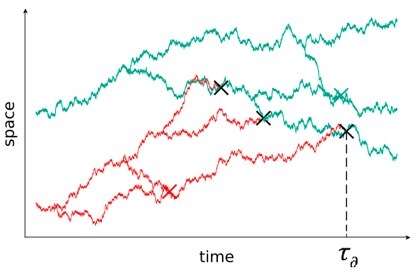
Our new observation here is that the quasi-stationary behavior of the stochastic FKPP is intimately related to that of the 2-type BCBM prior to the stopping time τ\tau_{\partial} defined in Definition 3.2 below. We declare this 22-type particle system to be “killed” when there are no more red particles, and consider the QSD of this 22-type particle system prior to be the “killing time” τ\tau_{\partial}. For tτt\geq\tau_{\partial}, there are no red particles while the green particles continue to evolve as a system of branching-coalescing Brownian motions. See Figure 1 for an illustration.

Refer to caption
Figure 1: A trajectory of the 2-type branching-coalescing Brownain motions (2-type BCBM) starting with one green particle and one red particle, where τ\tau_{\partial} is the first time when all red particles die off.

Indeed, since red particles cannot reappear once they disappear, {(G,R):R=}\{(G,R):R=\emptyset\} is a cemetery set. The 22-type BCBM with the absorption time τ\tau_{\partial} therefore defines an absorbed (or killed) Markov process, which we call the killed 22-type BCBM and denote as (Zt)0t<τ(Z_{t})_{0\leq t<\tau_{\partial}}. We will always assume that the 2-type BCBCM starts with at least one green particle and at least one red particle. Then the killed 2-type BCBM prior to killing has state space

χ:=(n1𝕊n/)×(m1𝕊m/),\chi:=(\cup_{n\geq 1}\mathbb{S}^{n}/\sim)\times(\cup_{m\geq 1}\mathbb{S}^{m}/\sim), (3.3)

where \sim is the equivalence relationship on 𝕊n\mathbb{S}^{n} such that x=(x1,,xn)x=(x1,,xn)x=(x_{1},\ldots,x_{n})\sim x^{\prime}=(x^{\prime}_{1},\ldots,x^{\prime}_{n}) if xx can be obtained from xx^{\prime} by permuting the coordinates.

Definition 3.2.

We consider the first time that all the red particles are killed, namely

τ:=inf{t0:Rt=},\tau_{\partial}:=\inf\{t\geq 0:\,R_{t}=\emptyset\},

and we call it the killing time of the 2-type BCBM. This then defines the killed 22-type BCBM (Zt)0t<τ(Z_{t})_{0\leq t<\tau_{\partial}}. A Borel probability measure, φ𝒫(χ)\varphi\in\mathcal{P}(\chi), is called a quasi-stationary distribution (QSD) for the killed 22-type BCBM (Zt)0t<τ(Z_{t})_{0\leq t<\tau_{\partial}} if

𝐏φ(Zt|τ>t)=φ()fort0.{\bf P}_{\varphi}(Z_{t}\in\,\cdot\;|\,\tau_{\partial}>t)\,=\,\varphi(\cdot)\quad\text{for}\quad t\in\mathbb{R}_{\geq 0}. (3.4)

Next we will define a family of functions {z}zχ\{\mathcal{E}^{z}\}_{z\in\chi} which will serve as the dual functions between the killed processes, and which is large enough to characterise measures on 𝒞\mathcal{C}_{\ast}. For ff\in\mathcal{B}_{\ast} and z=(x,y)=((x1,,xn),(y1,,ym))χz=(x,y)=((x_{1},\ldots,x_{n}),(y_{1},\ldots,y_{m}))\in\chi, we define

(f,z):=\displaystyle\mathcal{E}(f,z):= D(f;x)D(f;(x,y))=[i=1n(1f(xi))][1j=1m(1f(yj))],\displaystyle\,D(f;x)-D(f;(x,y))=\,\Big{[}\prod_{i=1}^{n}(1-f(x_{i}))\Big{]}\Big{[}1-\prod_{j=1}^{m}(1-f(y_{j}))\Big{]}, (3.5)

where the function D(f;x¯):=i=1n(1f(xi))D(f;\bar{x}):=\prod_{i=1}^{n}\left(1-f(x_{i})\right) was defined in (3.2). We further define

z(f):=(f,z).\mathcal{E}^{z}(f):=\mathcal{E}(f,z).

We will apply Lemma 3.3 below to use {z}zχ\{\mathcal{E}^{z}\}_{z\in\chi} to characterize the QSD of the stochastic FKPP.

Lemma 3.3.

Suppose that μ1\mu_{1} and μ2\mu_{2} are finite non-negative measures on 𝒞\mathcal{C}_{\ast} such that μ1(z)=μ2(z)\mu_{1}(\mathcal{E}^{z})=\mu_{2}(\mathcal{E}^{z}) for all zχz\in\chi. Then μ1=μ2\mu_{1}=\mu_{2}.

The proof of this self-contained lemma is given in the Appendix.

Proposition 3.4.

(Duality between killed processes.) Let α,γ(0,)\alpha,\gamma\in(0,\infty) and β0\beta\in\mathbb{R}_{\geq 0} be fixed constants. Let uu be the stochastic FKPP and ZZ be the 2-type BCBM corresponding to these constants. It holds that for all ff\in\mathcal{B}_{\ast}, zχz\in\chi and t0t\in\mathbb{R}_{\geq 0},

𝔼f[z(ut)𝟙(τfix>t)]=𝐄z[Zt(f) 1(τ>t)],\mathbb{E}_{f}[\mathcal{E}^{z}(u_{t})\mathbbm{1}(\tau_{\text{fix}}>t)]={\bf E}_{z}[\mathcal{E}^{\,Z_{t}}(f)\,\mathbbm{1}(\tau_{\partial}>t)], (3.6)

where :×χ[0,1]\mathcal{E}:\,\mathcal{B}_{\ast}\times\chi\to[0,1] is the function defined in (3.5). In other words, (Ptz)(f)=(Qt(f))(z)(P_{t}\mathcal{E}^{z})(f)=\left(Q_{t}\mathcal{E}^{\bullet}(f)\right)(z), where {Qt}\{Q_{t}\} is the sub-Markovian transition semigroup of the killed 2-type BCBM, acting on the function zz(f)z\mapsto\mathcal{E}^{z}(f), and {Pt}\{P_{t}\} is the sub-Markovian transition semigroup of the killed stochastic FKPP.

Proof of Proposition 3.4.

We take u0(𝕊;[0,1])u_{0}\in\mathcal{B}(\mathbb{S};\,[0,1]) and zχz\in\chi fixed and arbitrary. The process (Zt)t0(Z_{t})_{t\in\mathbb{R}_{\geq 0}} is the usual (11-type) system of BCBMs starting from zz, if we ignore the color. Similarly we define (ut)t0(u_{t})_{t\in\mathbb{R}_{\geq 0}} to be the stochastic FKPP, defined for all time (so defined for tτfixt\geq\tau_{\text{fix}}). Therefore we have

𝔼u0[D(ut,z)]=(3.1)𝐄z[D(u0,Zt)].{\mathbb{E}}_{u_{0}}[D(u_{t},\,z)]\stackrel{{\scriptstyle(\ref{WFdual})}}{{=}}{\bf E}_{z}[D(u_{0},\,Z_{t})]. (3.7)

On the other hand, the subset GtG_{t} also constitutes a (11-type) system of BCBMs that is not affected by the red particles, hence

𝔼u0[D(ut,g)]=(3.1)𝐄g[D(u0;Gt)]=𝐄(g,r)[D(u0;Gt)].{\mathbb{E}}_{u_{0}}[D(u_{t},\,g)]\stackrel{{\scriptstyle(\ref{WFdual})}}{{=}}{\bf E}_{g}[D(u_{0};\,G_{t})]={\bf E}_{(g,r)}[D(u_{0};\,G_{t})]. (3.8)

Subtracting (3.7) from (3.8) and recalling (3.5), we obtain that for all zχz\in\chi we have

𝔼u0[(ut,z)]=𝐄z[(u0;Zt)].{\mathbb{E}}_{u_{0}}[\mathcal{E}(u_{t},\,z)]={\bf E}_{z}[\mathcal{E}(u_{0};\,Z_{t})]. (3.9)

If tτt\geq\tau_{\partial}, then (u0,Zt)=0\mathcal{E}(u_{0},Z_{t})=0 for all u0u_{0} because Gt=ZtG_{t}=Z_{t}. On the other hand, if tτfixt\geq\tau_{\text{fix}}, then (ut,z)=0\mathcal{E}(u_{t},z)=0 for all zχz\in\chi since ut0u_{t}\equiv 0 or ut1u_{t}\equiv 1. Therefore, (3.6) follows from (3.9). ∎

We define the sub-Markovian transition semigroup (Qt)t0(Q_{t})_{t\in\mathbb{R}_{\geq 0}} of the killed 22-type BCBM in the same manner as in the definition for the stochastic FKPP in (2.4), namely

Qt(z,):=𝐏z(Zt,τ>t),zχ,μQt():=𝐏μ(Zt,τ>t),μ𝒫(χ),Qtf(z):=𝐄z[f(Zt)𝟙(τ>t)],fb(χ).\begin{split}&Q_{t}(z,\cdot):=\,{\bf P}_{z}(Z_{t}\in\cdot,\tau_{\partial}>t),\quad z\in\chi,\\ &\mu Q_{t}(\cdot):=\,{\bf P}_{\mu}(Z_{t}\in\cdot,\tau_{\partial}>t),\quad\mu\in\mathcal{P}(\chi),\\ &Q_{t}f(z):=\,{\bf E}_{z}[f(Z_{t})\mathbbm{1}(\tau_{\partial}>t)],\quad f\in\mathcal{B}_{b}(\chi).\end{split} (3.10)

Then as with the stochastic FKPP, φ𝒫(χ)\varphi\in\mathcal{P}(\chi) is a quasi-stationary distribution for the killed 22-type BCBM if and only if it is a left eigenmeasure for (Qt)t0(Q_{t})_{t\geq 0}. As with (2.6), we write Λ(φ)\Lambda(\varphi) and Λ(ϕ)\Lambda(\phi) respectively for the eigenvalues of a QSD φ\varphi and a right eigenfunction ϕ\phi, so that

φQt=(Λ(φ))tφ,Qtϕ=(Λ(ϕ))tϕ,t0.\varphi Q_{t}=(\Lambda(\varphi))^{t}\varphi,\quad Q_{t}\phi=(\Lambda(\phi))^{t}\phi,\quad t\geq 0. (3.11)

Analogously to Theorems 2.1 and 2.3 for the stochastic FKPP, we have Theorems 3.5 and 3.6 respectively for the dual process.

Theorem 3.5.

The killed 22-type BCBM (Zt)0t<τ(Z_{t})_{0\leq t<\tau_{\partial}} has a unique quasi-stationary distribution φ𝒫(χ)\varphi\in\mathcal{P}(\chi). Furthermore, we have the convergence

𝐏ν(Zt|τ>t)φ()in total variation{\bf P}_{\nu}(Z_{t}\in\,\cdot\;|\,\tau_{\partial}>t)\,\to\,\varphi(\cdot)\quad\text{in total variation} (3.12)

as tt\to\infty, for any initial condition ν𝒫(χ)\nu\in\mathcal{P}(\chi).

Recall that 𝒞b(χ;>0)\mathcal{C}_{b}(\chi;\mathbb{R}_{>0}) is the space of bounded, continuous, everywhere strictly positive function on χ\chi.

Theorem 3.6.

There exists ϕ𝒞b(χ;>0)\phi\in\mathcal{C}_{b}(\chi;\mathbb{R}_{>0}) which is a right eigenfunction of the killed 22-type BCBM (Zt)0t<τ(Z_{t})_{0\leq t<\tau_{\partial}} with the same positive eigenvalue as the unique QSD, Λ(ϕ)=Λ(φ)(0,1)\Lambda(\phi)=\Lambda(\varphi)\in(0,1). Moreover ϕ\phi is the unique (up to constant multiple) right eigenfunction of (Zt)0t<τ(Z_{t})_{0\leq t<\tau_{\partial}} in b(χ;>0)\mathcal{B}_{b}(\chi;\mathbb{R}_{>0}). Furthermore the right eigenfunction ϕ\phi and eigenvalue λ:=Λ(ϕ)\lambda:=\Lambda(\phi) give the leading-order asymptotics of the killing time for any initial condition, in the sense that

λt𝐏ν(τ>t)ν(ϕ)φ(ϕ)\lambda^{-t}{\bf P}_{\nu}(\tau_{\partial}>t)\rightarrow\frac{\nu(\phi)}{\varphi(\phi)} (3.13)

as tt\to\infty, for any initial condition ν𝒫(χ)\nu\in\mathcal{P}(\chi).

The QSDs and the right eigenfunctions of the two processes (the stochastic FKPP and the 2-type BCBM) are related as follows. Let :×χ[0,1]\mathcal{E}:\,\mathcal{B}_{\ast}\times\chi\to[0,1] be defined in (3.5). Define the functions Φ:χ\Phi:\,\chi\to\mathbb{R} and H:H:\,\mathcal{B}_{\ast}\to\mathbb{R} by

Φ(z):=Φπ(z):=𝒞z(f)π(df),zχ\Phi(z):=\Phi_{\pi}(z):=\int_{\mathcal{C}_{\ast}}\mathcal{E}^{z}(f)\,\pi(df),\qquad z\in\chi (3.14)

and

H(f):=Hφ(f):=χz(f)φ(dz),f.H(f):=H_{\varphi}(f):=\int_{\chi}\mathcal{E}^{z}(f)\,\varphi(dz),\qquad f\in\mathcal{B}_{\ast}. (3.15)

By Tonelli’s theorem,

π(H)=φ(Φ)=𝒞χz(f)φ(dz)π(df).\pi(H)=\varphi(\Phi)=\int_{\mathcal{C}_{\ast}}\int_{\chi}\mathcal{E}^{z}(f)\varphi(dz)\pi(df). (3.16)
Theorem 3.7.

(QSD and eigenfunction of the dual) Let u=(ut)0t<τfixu=(u_{t})_{0\leq t<\tau_{\text{fix}}} be the killed stochastic FKPP and (Zt)0t<τ(Z_{t})_{0_{\leq t<\tau_{\partial}}} the killed 2-type BCBM corresponding to a given set of constants α(0,)\alpha\in(0,\infty), β0\beta\in\mathbb{R}_{\geq 0} and γ0\gamma\in\mathbb{R}_{\geq 0}. Let π\pi and φ\varphi be the QSDs of uu and ZZ respectively, mentioned in Theorems 2.1 and 3.5. The following holds:

  1. 1.

    The function Φ\Phi defined in (3.14) belongs to 𝒞b(χ;>0)\mathcal{C}_{b}(\chi;\mathbb{R}_{>0}) and is the unique non-negative right eigenfunction (up to constant multiple) of the the killed 22-type BCBM.

  2. 2.

    The function HH defined in (3.15) belongs to 𝒞b(;>0)\mathcal{C}_{b}(\mathcal{B}_{\ast};\mathbb{R}_{>0}) and is the unique non-negative right eigenfunction (up to constant multiple) of the killed stochastic FKPP.

  3. 3.

    These QSDs and right eigenfunctions all share the same eigenvalue; that is,

    Λ(π)=Λ(H)=Λ(φ)=Λ(Φ)(0,1).\Lambda(\pi)=\Lambda(H)=\Lambda(\varphi)=\Lambda(\Phi)\in(0,1). (3.17)

Unless otherwise stated, we always normalize the right eigenfunctions by taking ϕ=Φ\phi=\Phi and h=Hh=H defined in (3.14) and (3.15) respectively. We summarize Theorem 3.7 and some related notations for the two processes in Table 1.

stochastic FKPP 2-type BCBM
the process u=(ut)t0u=(u_{t})_{t\in\mathbb{R}_{\geq 0}} Zt=(Gt,Rt),t0Z_{t}=(G_{t},R_{t}),\;t\in\mathbb{R}_{\geq 0}
killing time τfix=inf{t0:ut=0or1}\tau_{\rm fix}=\inf\{t\in\mathbb{R}_{\geq 0}:u_{t}=\textbf{0}\;\text{or}\;\textbf{1}\} τ=inf{t0:Rt=}\tau_{\partial}=\inf\{t\in\mathbb{R}_{\geq 0}:\,R_{t}=\emptyset\}
state space prior killing :=(𝕊;[0,1])(0¯1¯)\mathcal{B}_{\ast}:=\mathcal{B}(\mathbb{S};[0,1])\setminus(\bar{\textbf{0}}\cup\bar{\textbf{1}}) χ=(n1𝕊n/)×(m1𝕊m/)\chi=(\cup_{n\geq 1}\mathbb{S}^{n}/\sim)\times(\cup_{m\geq 1}\mathbb{S}^{m}/\sim)
sub-Markovian kernel Pt(f,)P_{t}(f,\cdot) for f,t0f\in\mathcal{B}_{\ast},\,t\in\mathbb{R}_{\geq 0} Qt(z,)Q_{t}(z,\cdot) for zχ,t0z\in\chi,\,t\in\mathbb{R}_{\geq 0}
QSD π𝒫(𝒞)\pi\in\mathcal{P}(\mathcal{C}_{\ast}) φ𝒫(χ)\varphi\in\mathcal{P}(\chi)
right eigenfunction h(f)=χ(f,z)φ(dz)=φ((f,))h(f)=\int_{\chi}\mathcal{E}(f,z)\,\varphi(dz)=\varphi(\mathcal{E}(f,\cdot)) ϕ(z)=𝒞(f,z)π(df)=π(z)\phi(z)=\int_{\mathcal{C}_{\ast}}\mathcal{E}(f,z)\,\pi(df)=\pi(\mathcal{E}^{z})
eigenvalue Λ(π)=Λ(h)\Lambda(\pi)=\Lambda(h) Λ(φ)=Λ(ϕ)\Lambda(\varphi)=\Lambda(\phi)
Table 1: Notation for the stochastic FKPP (1.1) and the 2-type branching-coalescing Brownian motion (Definition 3.1). We allow the initial condition of the stochastic FKPP to belong to the space \mathcal{B}_{\ast} which is larger than 𝒞:=𝒞(𝕊;[0,1]){0,1}\mathcal{C}_{\ast}:=\mathcal{C}(\mathbb{S};[0,1])\setminus\{{\textbf{0}},{\textbf{1}}\}. The function :×χ[0,1]\mathcal{E}:\,\mathcal{B}_{*}\times\chi\to[0,1] is defined in (3.5). We have π(h)=φ(ϕ)\pi(h)=\varphi(\phi) by (3.16).

The proofs of Theorems 2.1, 2.3, 3.5, 3.6 and 3.7 will be given in Sections 5-6. Before this, in Section 4, we present some explicit calculations for the case β=0\beta=0 that may offer some insights for the quasi-stationary behavior of the stochastic FKPP. None of our proofs in Sections 5-6 (nor in the Appendix) depend on any calculation in Section 4.

4 Explicit calculations when β=0\beta=0

This section aims to offer explicit insights of our general results, and can be skipped if the reader is interested only in the proofs of Theorems 2.1, 2.3, 3.5, 3.6 and 3.7 at this point.

Recall from (3.14) that ϕ(z)=𝒞z(f)π(df)\phi(z)=\int_{\mathcal{C}_{\ast}}\mathcal{E}^{z}(f)\,\pi(df) is the unique (up to a constant multiple) right engenfunction of the killed 2-type BCBM. Hence, in principle, all moments of the QSD π\pi of the stochastic FKPP can be computed from the right eigenfunction ϕ\phi of the 2-type BCBM, and these moments uniquely determine π\pi, by Lemma 3.3. As in the well-mixed case (Section A.4), explicit calculations for the QSD are only possible when β=0\beta=0.

We note, however, that a general approximation method for killed Markov processes based on interacting particle systems has been established by Villemonais [Vil14], having been originally introduced in the case of Brownian dynamics by Burdzy, Hołyst and March [BHM00]. This may be employed to numerically sample the QSD of the 22-type killed BCBM with β>0\beta>0, providing numerics for the fixation time of the stochasic FKPP by the duality established in Section 3.

For the rest of this section, we assume that β=0\beta=0, while α,γ>0\alpha,\gamma\in\mathbb{R}_{>0} are fixed and arbitrary. Since β=0\beta=0, there is no branching and the 22-type branching-coalescing Brownian motion is simply a 22-type coalescing Brownian motion (CBM).

4.1 QSD and eigenpair for the 22-type CBM

Recall from Theorem 3.5 that the 22-type CBM Z=(G,R)Z=(G,R) with β=0\beta=0 has a unique QSD φ0\varphi^{0}. As we shall see in Proposition 5.2, φ0\varphi^{0} is supported on 𝕊×𝕊\mathbb{S}\times\mathbb{S} and that has a density function with respect to Lebesgue measure. We further recall from Theorems 3.6 and 3.7 that the killed 22-type CBM has a unique (up to constant multiple) right eigenfunction ϕ0𝒞b(χ;>0)\phi^{0}\in\mathcal{C}_{b}(\chi;\mathbb{R}_{>0}) which has the same eigenvalue as the QSD, Λ(ϕ0)=Λ(φ0)\Lambda(\phi^{0})=\Lambda(\varphi^{0}).

In Theorem 4.1, we explicitly write down the QSD φ0\varphi^{0} and the right eigenfunction ϕ0\phi^{0}, and their common eigenvalue. Equation (4.3) gives the restriction of ϕ0\phi^{0} to 𝕊×𝕊\mathbb{S}\times\mathbb{S}, which is more explicit than the representation (4.4) of ϕ0\phi^{0} on its domain χ\chi.

Theorem 4.1 (QSD and eigenpair for the 2-type CBM).

We suppose that β=0\beta=0. Let θ(0,π2)\theta_{\ast}\in\big{(}0,\frac{\pi}{2}\big{)} be the unique solution to

γα=4θtan(θ).\frac{\gamma}{\alpha}=4\theta\tan(\theta). (4.1)

Then the unique QSD φ0\varphi^{0} of the killed 22-type CBM ZZ is an element of 𝒫(𝕊×𝕊)\mathcal{P}(\mathbb{S}\times\mathbb{S}) and is explicitly given by φ0(dx,dy)=ρ0(x,y)dxdy\varphi^{0}(dx,dy)=\rho^{0}(x,y)\,dxdy, whereby

ρ0(x,y)=θsin(θ)cos(2θ(12d𝕊(x,y))).\rho^{0}(x,y)=\frac{\theta_{\ast}}{\sin(\theta_{\ast})}\cos\Big{(}2\theta_{\ast}\Big{(}\frac{1}{2}-d_{\mathbb{S}}(x,y)\Big{)}\Big{)}. (4.2)

Let ϕ0𝒞b(χ;>0)\phi^{0}\in\mathcal{C}_{b}(\chi;\mathbb{R}_{>0}) be the right eigenfunction of the 22-type CBM given by (3.14). The restriction of ϕ0\phi^{0} to 𝕊×𝕊\mathbb{S}\times\mathbb{S} is equal to

ϕ|𝕊×𝕊0((x,y))=Mcos(2θ(12d𝕊(x,y))),\phi^{0}_{\lvert_{\mathbb{S}\times\mathbb{S}}}((x,y))=M_{*}\cos\Big{(}2\theta_{\ast}\Big{(}\frac{1}{2}-d_{\mathbb{S}}(x,y)\Big{)}\Big{)}, (4.3)

where M(0,)M_{*}\in(0,\infty) is a constant. Furthermore,

ϕ0(z)=Mcos(θ)𝐄z[e4αθ2τZ]forzχ,\phi^{0}(z)=M_{\ast}\cos(\theta_{\ast})\,{\bf E}_{z}\left[e^{4\alpha\theta_{\ast}^{2}\tau^{Z}}\right]\quad\text{for}\quad z\in\chi, (4.4)

where τZ\tau^{Z} is the first time that ZZ consists of one green particle and one red particle, both at the same position. The common eigenvalue λ\lambda of φ0\varphi^{0} and of ϕ0\phi^{0} is given by

λ=Λ(ϕ0)=Λ(φ0)=e4αθ2.\lambda=\Lambda(\phi^{0})=\Lambda(\varphi^{0})=e^{-4\alpha\theta_{\ast}^{2}}. (4.5)

The constant MM_{*} in (4.3) will be determined in (4.9) below in terms of the usual 11-type coalescing Brownian motion (CBM) X¯\bar{X} mentioned in 3.1. We define τ1\tau_{1} to be the first time when X¯\bar{X} consists of exactly two particles both at the same position. That is,

τ1:=inf{t0:|t|=2,Xti=Xtj whenever i,jt}.\tau_{1}:=\inf\{t\in\mathbb{R}_{\geq 0}:\,|\mathcal{I}_{t}|=2,\;X^{i}_{t}=X^{j}_{t}\text{ whenever }i,j\in\mathcal{I}_{t}\}. (4.6)

Given a closed set F𝕊F\subseteq\mathbb{S}, we define ΣF\Sigma_{F} to be the set of infinite sequences in 𝕊\mathbb{S} whose closure and limit set (i.e. the set of accumulation points) are both given by FF. That is,

ΣF:={x¯:=(x1,x2,)F:every xF is an accumulation point of x¯}.\Sigma_{F}:=\{\underline{x}:=(x_{1},x_{2},\ldots)\in F^{\mathbb{N}}:\;\text{every $x^{\prime}\in F$ is an accumulation point of $\underline{x}$}\}. (4.7)

For instance, Σ{0,12}={(0,0,)}{(12,12,)}\Sigma_{\{0,\,\frac{1}{2}\}}=\{(0,0,\ldots)\}\cup\{(\frac{1}{2},\frac{1}{2},\ldots)\}, while Σ𝕊\Sigma_{\mathbb{S}} consists of all dense sequences in 𝕊\mathbb{S}.

Lemma 4.2.

Suppose β=0\beta=0. Let FF be a closed and non-empty subset of 𝕊\mathbb{S}. Then the limit

𝐄x¯[e4αθ2τ1]:=limn𝐄(xi)i=1n[e4αθ2τ1]{\bf E}_{\bar{x}}\left[e^{4\alpha\theta_{\ast}^{2}\tau_{1}}\right]:=\lim_{n\to\infty}{\bf E}_{(x_{i})_{i=1}^{n}}\left[e^{4\alpha\theta_{\ast}^{2}\tau_{1}}\right]

exists in (1,)(1,\infty). This number is the same for all x¯=(x1,x2,)ΣF\underline{x}=(x_{1},x_{2},\ldots)\in\Sigma_{F}, hence we can denote it by 𝐄F[e4αθ2τ1]{\bf E}_{F}\left[e^{4\alpha\theta_{\ast}^{2}\tau_{1}}\right]. Furthermore, the strict inequality

𝐄F[e4αθ2τ1]<𝐄F[e4αθ2τ1]{\bf E}_{F}\left[e^{4\alpha\theta_{\ast}^{2}\tau_{1}}\right]<{\bf E}_{F^{\prime}}\left[e^{4\alpha\theta_{\ast}^{2}\tau_{1}}\right] (4.8)

holds for all non-empty, closed subsets FF and FF^{\prime} such that FF𝕊\emptyset\neq F\subsetneq F^{\prime}\subseteq\mathbb{S}.

In particular, the limit 𝐄x¯[e4αθ2τ1](1,){\bf E}_{\bar{x}}\left[e^{4\alpha\theta_{\ast}^{2}\tau_{1}}\right]\in(1,\infty) does not depend upon the choice of x¯Σ𝕊\underline{x}\in\Sigma_{\mathbb{S}}, and is denoted by 𝐄𝕊[e4αθ2τ1]{\bf E}_{\mathbb{S}}\left[e^{4\alpha\theta_{\ast}^{2}\tau_{1}}\right].

Theorem 4.3.

When ϕ0\phi^{0} is given by (3.14), the constant MM_{*} in (4.3) is equal to

M:=12cos(θ)𝐄𝕊[e4αθ2τ1](0,).M_{\ast}:=\frac{1}{2\cos(\theta_{\ast})\,{\bf E}_{\mathbb{S}}\left[e^{4\alpha\theta_{\ast}^{2}\tau_{1}}\right]}\in(0,\infty). (4.9)

4.2 QSD and eigenpair for neutral FKPP

We now apply Theorem 4.1 to the neutral stochastic FKPP. Immediately from Theorem 3.7, the eigenvalue of π0\pi^{0} and h0h^{0} is equal to

λ:=Λ(π0)=Λ(h0)=e4αθ2.\lambda:=\Lambda(\pi^{0})=\Lambda(h^{0})=e^{-4\alpha\theta_{\ast}^{2}}. (4.10)

It follows that the fixation rate, defined as κ=lnλ\kappa=-\ln\lambda, is given by

κ=4αθ2.\kappa=4\alpha\theta_{\ast}^{2}. (4.11)

By (2.7) in Theorem 2.3, the leading order asymptotics of the fixation time is given, for each uu\in\mathcal{B}_{\ast}, by

u(τfix>t)(2.7)\displaystyle\mathbb{P}_{u}(\tau_{\text{fix}}>t)\stackrel{{\scriptstyle(\ref{AbsTime_1})}}{{\sim}} e4αθ2th0(u)π0(h0)as t,\displaystyle\,e^{-4\alpha\theta_{\ast}^{2}\,t}\,\frac{h^{0}(u)}{\pi^{0}(h^{0})}\qquad\text{as }t\to\infty, (4.12)

where h0(u)h^{0}(u) and π0(h0)\pi^{0}(h^{0}) are given respectively by

h0(u)=(3.15)χz(u)φ0(dz)=(4.2)θsin(θ)𝕊×𝕊(1u(x))u(y)cos(2θ(12d𝕊(x,y)))𝑑x𝑑yh^{0}(u)\stackrel{{\scriptstyle(\ref{eq:formula for right efn of dual in terms of QSD of FKPP results})}}{{=}}\int_{\chi}\mathcal{E}^{z}(u)\,\varphi^{0}(dz)\stackrel{{\scriptstyle(\ref{eq:QSD density for 2-particle CBM})}}{{=}}\frac{\theta_{\ast}}{\sin(\theta_{\ast})}\int_{\mathbb{S}\times\mathbb{S}}(1-u(x))u(y)\cos\Big{(}2\theta_{\ast}\Big{(}\frac{1}{2}-d_{\mathbb{S}}(x,y)\Big{)}\Big{)}\,dx\,dy (4.13)

for uu\in\mathcal{B}_{\ast}, and

π0(h0)=(3.16)φ0(ϕ0)\displaystyle\pi^{0}(h^{0})\stackrel{{\scriptstyle(\ref{eq:duality theorem integral of right efns the same})}}{{=}}\varphi^{0}(\phi^{0}) =(4.3)𝕊×𝕊Mcos(2θ(12d𝕊(x,y)))φ0(dx,dy)\displaystyle\stackrel{{\scriptstyle(\ref{eq:expression for right e-fn of CBM})}}{{=}}\,\int_{\mathbb{S}\times\mathbb{S}}M_{*}\cos\Big{(}2\theta_{\ast}\Big{(}\frac{1}{2}-d_{\mathbb{S}}(x,y)\Big{)}\Big{)}\,\varphi^{0}(dx,dy) (4.14)
=(4.2)Mθsin(θ)𝕊×𝕊cos2(2θ(12d𝕊(x,y)))𝑑x𝑑y=Mθsin(θ)12(1+sin(2θ)2θ).\displaystyle\stackrel{{\scriptstyle(\ref{eq:QSD density for 2-particle CBM})}}{{=}}\,\frac{M_{*}\theta_{\ast}}{\sin(\theta_{\ast})}\,\int_{\mathbb{S}\times\mathbb{S}}\cos^{2}\Big{(}2\theta_{\ast}\Big{(}\frac{1}{2}-d_{\mathbb{S}}(x,y)\Big{)}\Big{)}\,dxdy=\,\frac{M_{*}\theta_{\ast}}{\sin(\theta_{\ast})}\,\frac{1}{2}\,\Big{(}1+\frac{\sin(2\theta_{\ast})}{2\theta_{\ast}}\Big{)}. (4.15)
Refer to caption
Figure 2: (Left) the eigenvalue λ=e4αθ2\lambda=e^{-4\alpha\theta_{\ast}^{2}} in (4.5) against α\alpha for fixed values of γ\gamma. The eigenvalue λ\lambda tends to eγe^{-\gamma} as α\alpha\uparrow\infty. (Right) the fixation rate κ=lnλ=4αθ2\kappa=-\ln\lambda=4\alpha\theta_{\ast}^{2} against α\alpha for fixed values of γ\gamma. It increases to γ\gamma (the fixation rate of the well-mixed case) as α\alpha\uparrow\infty and it decreases to 0 as α0\alpha\downarrow 0.

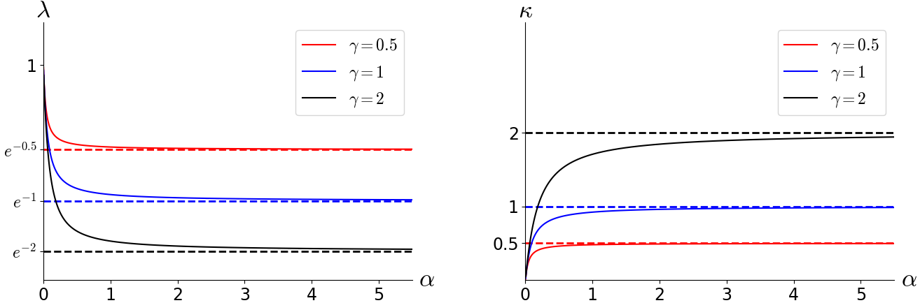
In Figure 2 (right), we plot the value of the fixation rate κ=lnλ\kappa=-\ln\lambda as a function of the diffusion constant α\alpha. By (4.1), we obtain the asymptotic expansions

κ={γ[1γ12α+γ2180α2γ33780α3+𝒪γα0(γ4α4)]asγα0(fast diffusion)π2α[18αγ+48α2γ2+𝒪αγ0(α3γ3)]asαγ0(slow diffusion)\kappa=\begin{dcases}\gamma\,\Big{[}1-\frac{\gamma}{12\alpha}+\frac{\gamma^{2}}{180\alpha^{2}}-\frac{\gamma^{3}}{3780\alpha^{3}}+\mathcal{O}_{\frac{\gamma}{\alpha}\rightarrow 0}\Big{(}\frac{\gamma^{4}}{\alpha^{4}}\Big{)}\Big{]}\qquad&\text{as}\quad\frac{\gamma}{\alpha}\to 0\qquad\text{(fast diffusion)}\\ \pi^{2}\alpha\,\Big{[}1-8\frac{\alpha}{\gamma}+48\frac{\alpha^{2}}{\gamma^{2}}+\mathcal{O}_{\frac{\alpha}{\gamma}\rightarrow 0}\Big{(}\frac{\alpha^{3}}{\gamma^{3}}\Big{)}\Big{]}\qquad&\text{as}\quad\frac{\alpha}{\gamma}\to 0\qquad\text{(slow diffusion)}\end{dcases} (4.16)

We observe that when γα\gamma\ll\alpha (fast diffusion), the fixation rate is determined to leading order only by γ\gamma, whereas when γα\gamma\gg\alpha (slow diffusion), the fixation rate is determined to leading order only by α\alpha.

Remark 4.4 (Faster spatial movement speeds up fixation).

From Figure 2 and (4.16), we see that faster spatial movement speeds up fixation, but there is an upper bound. As the diffusion coefficient α\alpha\uparrow\infty, the fixation rate κ\kappa of the stochastic FKPP increases to γ\gamma which agrees with the fixation rate in the well-mixed case (1.5), and for a large but finite diffusion constant α\alpha, the fixation rate is smaller by about γ212α\frac{\gamma^{2}}{12\alpha} and so it takes a longer time to get to fixation compared with the well-mixed case in the sense of (4.12). On other hand, as α0\alpha\downarrow 0, the fixation rate κ\kappa decreases to 0 like π2α\pi^{2}\alpha. The constants 112\frac{1}{12} and π2\pi^{2} may change if the circle is changed to other spaces on which the stochastic FKPP admits a solution [Fan20]; we do not know. How fixation rate changes in terms of the geometry of the underlying space is of considerable interest in population genetics.

We now use Theorem 4.1 to obtain some explicit calculations for the QSD π0\pi^{0}. We firstly note that by symmetry, 𝔼uπ0[u(x)]=12\mathbb{E}_{u\sim\pi^{0}}[u(x)]=\frac{1}{2} for all x𝕊x\in\mathbb{S}. We have from (3.14) and (4.3) that

𝔼uπ0[(1u(x))u(y)]=Mcos(2θ(12d𝕊(x,y))),x,y𝕊.\mathbb{E}_{u\sim\pi^{0}}[(1-u(x))u(y)]=M_{\ast}\cos\Big{(}2\theta_{\ast}\Big{(}\frac{1}{2}-d_{\mathbb{S}}(x,y)\Big{)}\Big{)},\quad x,y\in\mathbb{S}.

We may therefore immediately calculate the following:

𝔼uπ0[u(x)u(y)]=\displaystyle\mathbb{E}_{u\sim\pi^{0}}[u(x)u(y)]= 12Mcos(2θ(12d𝕊(x,y))),x,y𝕊,\displaystyle\frac{1}{2}-M_{\ast}\cos\Big{(}2\theta_{\ast}\Big{(}\frac{1}{2}-d_{\mathbb{S}}(x,y)\Big{)}\Big{)},\quad x,y\in\mathbb{S}, (4.17)
Covuπ0(u(x),u(y))=\displaystyle\text{Cov}_{u\sim\pi^{0}}(u(x),u(y))= 14Mcos(2θ(12d𝕊(x,y))),x,y𝕊,\displaystyle\frac{1}{4}-M_{\ast}\cos\Big{(}2\theta_{\ast}\Big{(}\frac{1}{2}-d_{\mathbb{S}}(x,y)\Big{)}\Big{)},\quad x,y\in\mathbb{S}, (4.18)
Var(𝕊u(x)𝑑x)=\displaystyle\text{Var}\Big{(}\int_{\mathbb{S}}u(x)dx\Big{)}= 14Msin(θ)θ.\displaystyle\frac{1}{4}-\frac{M_{\ast}\sin(\theta_{\ast})}{\theta_{\ast}}. (4.19)

Local fixation. Our next result implies that for any non-empty disjoint closed sets F1,F2𝕊F_{1},\,F_{2}\subset\mathbb{S}, local fixation can occur on F1F_{1} but not on F2F_{2} under the QSD of the neutral stochastic FKPP. This represents the event that there is no genetic diversity on a region F1F_{1}, while there is genetic variation on F2F_{2}.

Definition 4.5.

Given f𝒞(𝕊;[0,1])f\in\mathcal{C}(\mathbb{S};[0,1]) and a non-empty closed set F𝕊F\subseteq\mathbb{S}, we say that ff is fixed on FF if f0f\equiv 0 on FF or f1f\equiv 1 on FF.

By the definition of the QSD, uπ0(u is not fixed on 𝕊)=1\mathbb{P}_{u\sim\pi^{0}}(u\text{ is not fixed on $\mathbb{S}$})=1. As we shall see in section 6.3, the strict inequalities (between 0 and 1) in Theorem 4.6 follow from (4.8).

Theorem 4.6 (Local fixation).

Suppose that β=0\beta=0. For any non-empty closed set F𝕊F\subsetneq\mathbb{S}, the probability that the neutral stochastic FKPP not being fixed on FF, under the quasi-stationary distribution π0\pi^{0}, is given by

uπ0(u is not fixed on F)=𝐄F[e4αθ2τ1]𝐄𝕊[e4αθ2τ1](0,1).\mathbb{P}_{u\sim\pi^{0}}(u\text{ is not fixed on $F$})=\frac{{\bf E}_{F}\left[e^{4\alpha\theta_{\ast}^{2}\tau_{1}}\right]}{{\bf E}_{\mathbb{S}}\left[e^{4\alpha\theta_{\ast}^{2}\tau_{1}}\right]}\in(0,1). (4.20)

Moreover, for all non-empty closed subsets FF and FF^{\prime} of 𝕊\mathbb{S} such that FFF\subsetneq F^{\prime}, it holds that

(u is fixed on F and not fixed on F)(0,1).\mathbb{P}(\text{$u$ is fixed on $F$ and not fixed on $F^{\prime}$})\in(0,1). (4.21)

Observe that (4.20) is equivalent to

uπ0(u0 on F)=12(1𝐄F[e4αθ2τ1]𝐄𝕊[e4αθ2τ1]),\mathbb{P}_{u\sim\pi^{0}}(u\equiv 0\text{ on $F$})=\frac{1}{2}\left(1-\frac{{\bf E}_{F}\left[e^{4\alpha\theta_{\ast}^{2}\tau_{1}}\right]}{{\bf E}_{\mathbb{S}}\left[e^{4\alpha\theta_{\ast}^{2}\tau_{1}}\right]}\right), (4.22)

because uπ0(u0 on F)=uπ0(u1 on F)\mathbb{P}_{u\sim\pi^{0}}(u\equiv 0\text{ on $F$})=\mathbb{P}_{u\sim\pi^{0}}(u\equiv 1\text{ on $F$}) by symmetry.

The strict inequalities in Theorem 4.6 offer some information about the support of the QSD π0\pi^{0}. For example, for any given non-empty closed set FF, π0\pi^{0} puts positive mass on paths that are fixed on FF. In particular,

uπ0(0<u(x)<1 for all x𝕊)[0,1).\mathbb{P}_{u\sim\pi^{0}}(0<u(x)<1\text{ for all }x\in\mathbb{S})\in[0,1).

Moreover, since m{x𝕊:u(x)=0}=limn𝕊(1u(x))nm(dx)m\{x\in\mathbb{S}:\,u(x)=0\}=\lim_{n\to\infty}\int_{\mathbb{S}}(1-u(x))^{n}\,m(dx) for each u𝒞u\in\mathcal{C}_{*}, we have

𝔼uπ0[m{x𝕊:u(x)=0}]=\displaystyle{\mathbb{E}}_{u\sim\pi^{0}}\left[m\{x\in\mathbb{S}:\,u(x)=0\}\right]= 𝕊uπ0(u(x)=0)m(dx)=uπ0(u(0)=0)\displaystyle\,\int_{\mathbb{S}}{\mathbb{P}}_{u\sim\pi^{0}}(u(x)=0)\,m(dx)={\mathbb{P}}_{u\sim\pi^{0}}(u(0)=0)
=\displaystyle= 12(1𝐄{0}[e4αθ2τ1]𝐄𝕊[e4αθ2τ1])(0, 1/2)\displaystyle\,\frac{1}{2}\left(1-\frac{{\bf E}_{\{0\}}\left[e^{4\alpha\theta_{\ast}^{2}\tau_{1}}\right]}{{\bf E}_{\mathbb{S}}\left[e^{4\alpha\theta_{\ast}^{2}\tau_{1}}\right]}\right)\in\left(0,\,1/2\right)

where the last equality follows from (4.22) with F={0}F=\{0\}.

Our results and methods lay the foundation for the study of detailed properties of the QSD for the stochastic FKPP. In particular, the technique in our proof of Theorem 4.6 enables us to obtain further properties of the QSD π0\pi^{0}. For example, for any closed disjoint subsets Fg,Fr𝕊F_{g},\,F_{r}\subset\mathbb{S},

uπ0({u0 on Fg}{u0 on Fr})=Mcos(θ)𝐄(x¯,y¯)[e4αθ2τZ],{\mathbb{P}}_{u\sim\pi^{0}}\left(\{u\equiv 0\text{ on $F_{g}$}\}\setminus\{u\equiv 0\text{ on $F_{r}$}\}\right)=M_{\ast}\cos(\theta_{\ast})\,{\bf E}_{(\underline{x},\underline{y})}[e^{4\alpha\theta_{\ast}^{2}\tau^{Z}}], (4.23)

where τZ\tau^{Z} is the first time that the 2-type CBM ZZ consists of one green and one red particle, both at the same position. The elements x¯=(x1,)ΣFg\underline{x}=(x_{1},\ldots)\in\Sigma_{F_{g}} and y¯=(y1,)ΣFr\underline{y}=(y_{1},\ldots)\in\Sigma_{F_{r}} are arbitrarily fixed and will not affect the value of 𝐄(x¯,y¯)[e4αθ2τZ]:=limn𝐄z(n)[e4αθ2τZ]{\bf E}_{(\underline{x},\underline{y})}[e^{4\alpha\theta_{\ast}^{2}\tau^{Z}}]:=\lim_{n\to\infty}{\bf E}_{z^{(n)}}[e^{4\alpha\theta_{\ast}^{2}\tau^{Z}}], where z(n):=((x1,xn),(y1,yn))z^{(n)}:=((x_{1}\ldots,x_{n}),\,(y_{1}\ldots,y_{n})).

A martingale. The duality that the coalescing Brownian motion enjoys with the neutral stochastic FKPP is a spatial version of the duality that Kingman’s coalescent enjoys with Wright-Fisher diffusion; the coalescing Brownian motion can be viewed as a spatial version of Kingman’s coalescent. Writing NtN_{t} for the number of blocks (or lineages) that Kingman’s coalescent has at time tt, it is well-known and easy to check that

et(121Nt+1)is a martingale.e^{t}\Big{(}\frac{1}{2}-\frac{1}{N_{t}+1}\Big{)}\quad\text{is a martingale.} (4.24)

We recover the corresponding martingale for coalescing Brownian motion in the following.

Corollary 4.7.

Suppose that X¯t:=(Xt1,,XtNt)\bar{X}_{t}:=(X^{1}_{t},\ldots,X^{N_{t}}_{t}) is a system of coalescing Brownian motion (described before (3.1) with β=0\beta=0). Then

e4αθ2t(12𝔼uπ0[i=1Nt(1u(Xti))])is a martingale.e^{4\alpha\theta_{\ast}^{2}t}\Big{(}\frac{1}{2}-\mathbb{E}_{u\sim\pi^{0}}\Big{[}\prod_{i=1}^{N_{t}}(1-u(X_{t}^{i}))\Big{]}\Big{)}\quad\text{is a martingale.} (4.25)

Indeed, it is well-known that the standard Wright-Fisher diffusion on [0,1][0,1] prior to fixation (when it hits 0 or 11) has the QSD πWF=Unif((0,1))\pi^{\text{WF}}=\text{Unif}((0,1)) [Sen66]. The analogue of the term in brackets in (4.25) is therefore

12𝔼uunif((0,1))[(1u)Nt]=1201(1u)Nt𝑑u=121Nt+1.\frac{1}{2}-\mathbb{E}_{u\sim\text{unif}((0,1))}\Big{[}(1-u)^{N_{t}}\Big{]}=\frac{1}{2}-\int_{0}^{1}(1-u)^{N_{t}}du=\frac{1}{2}-\frac{1}{N_{t}+1}.

Therefore, (4.25) is the spatial version of (4.24).

5 Overview of the proofs of our main results

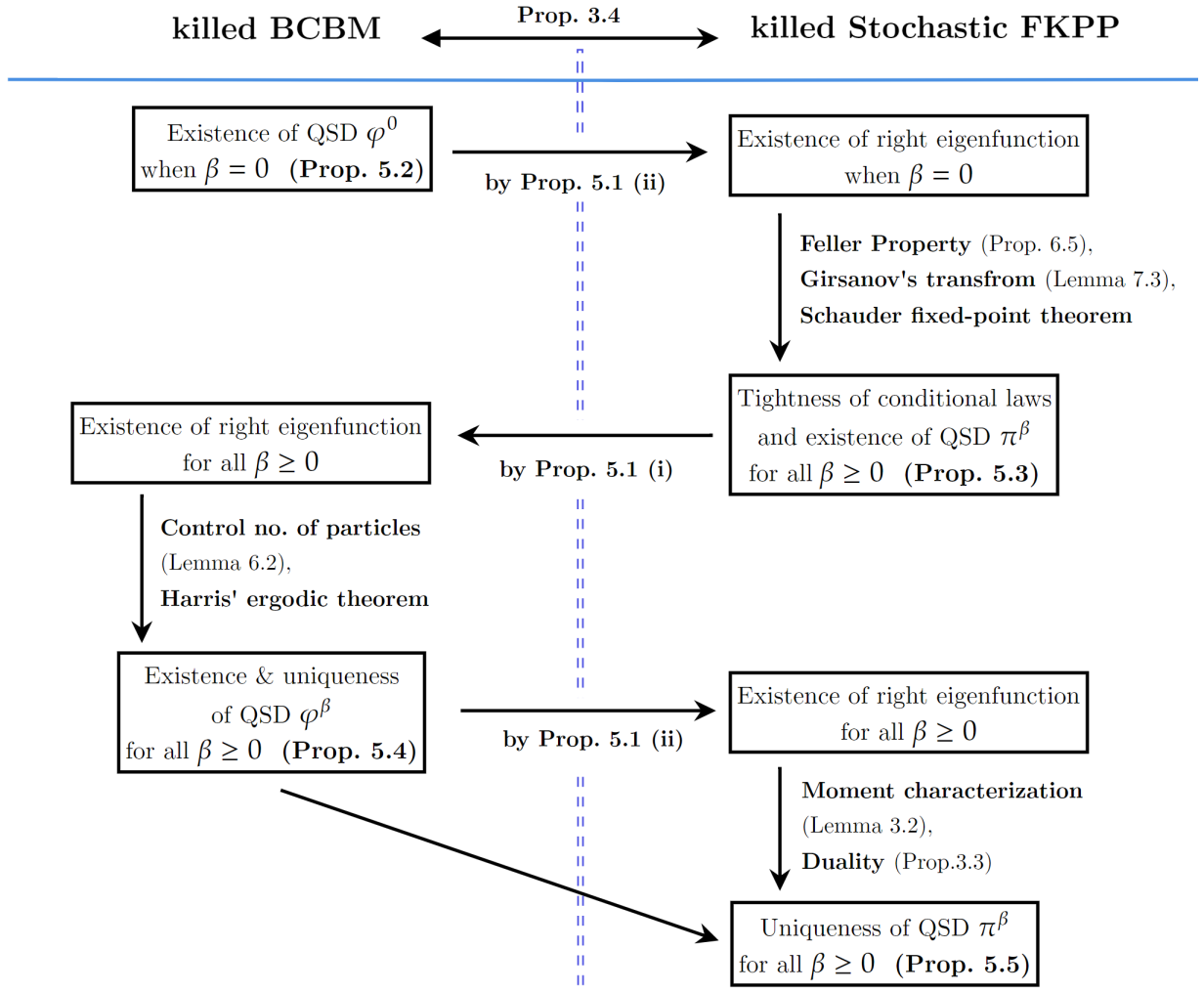
In this section, we provide an overview of our proofs. Our proofs will be decomposed into Propositions 5.1- 5.5, which we shall establish later, in turn, in Section 6.2. Assuming these propositions, we give the proofs of Theorems 2.1, 2.3, 3.5, 3.6 and 3.7 at the end of this section. The key ideas and structure of our proofs are laid out in Fig. 3.

Our first proposition establishes a general link between the killed stochastic FKPP and the killed 22-type BCBM, as in Theorem 3.7, without knowledge about uniqueness of QSDs or that of the right eigenfunctions.

Proposition 5.1 (QSD gives right eigenfunction of the dual).

Let u=(ut)0t<τfixu=(u_{t})_{0\leq t<\tau_{\text{fix}}} be the killed stochastic FKPP and (Zt)0t<τ(Z_{t})_{0_{\leq t<\tau_{\partial}}} the killed 2-type BCBM corresponding to a given set of constants α(0,)\alpha\in(0,\infty), β0\beta\in\mathbb{R}_{\geq 0} and γ0\gamma\in\mathbb{R}_{\geq 0}.

  1. (i)

    Suppose that π𝒫(𝒞)\pi\in\mathcal{P}(\mathcal{C}_{*}) is a quasi-stationary distribution for the stochastic FKPP and Λ(π)>0\Lambda(\pi)>0 is the corresponding left eigenvalue. Then ϕ(z):=𝒞z(f)π(df)\phi(z):=\int_{\mathcal{C}_{\ast}}\mathcal{E}^{z}(f)\,\pi(df) defined by (3.14) belongs to 𝒞b(χ;>0)\mathcal{C}_{b}(\chi;\mathbb{R}_{>0}) and is a right eigenfunction of the the killed 22-type BCBM. Furthermore, Λ(ϕ)=Λ(π)\Lambda(\phi)=\Lambda(\pi).

  2. (ii)

    Suppose that φ𝒫(χ)\varphi\in\mathcal{P}(\chi) is a QSD of the 22-type BCBM and Λ(φ)>0\Lambda(\varphi)>0 is the corresponding left eigenvalue. Then h(f):=χz(f)φ(dz)h(f):=\int_{\chi}\mathcal{E}^{z}(f)\,\varphi(dz) defined by (3.15) belongs to 𝒞b(;>0)\mathcal{C}_{b}(\mathcal{B}_{\ast};\mathbb{R}_{>0}) and is a right eigenfunction of the killed stochastic FKPP. Furthermore, Λ(h)=Λ(φ)\Lambda(h)=\Lambda(\varphi).

The starting point of our proof of Theorem 2.1 will be the key observation that, when β=0\beta=0, the dual process has a QSD that is supported on the finite dimensional space 𝒮×𝒮\mathcal{S}\times\mathcal{S}, enabling us to obtain various tightness results. Moreover this QSD is amenable to exact analysis, enabling the precise calculations of Section 4 (note that these precise calculations are not needed for the proofs of our main results). In the rest of the proof, it shall be necessary to vary β0\beta\in\mathbb{R}_{\geq 0}. Where necessary to avoid ambiguity, we indicate this by a superscript β\beta.

Proposition 5.2 (Existence of QSD for CBM when β=0\beta=0).

The 22-type CBM with β=0\beta=0 (i.e. without branching) has a QSD, denoted by φ0\varphi^{0}, which is supported on 𝕊×𝕊\mathbb{S}\times\mathbb{S}. The restriction φ|𝕊×𝕊Γ0\varphi^{0}_{\lvert_{\mathbb{S}\times\mathbb{S}\setminus\Gamma}} off the diagonal Γ:={(x,y)𝕊×𝕊:x=y}\Gamma:=\{(x,y)\in\mathbb{S}\times\mathbb{S}:x=y\} has a density with respect to Lebesgue measure which is an element of 𝒞(𝕊×𝕊Γ;>0)\mathcal{C}(\mathbb{S}\times\mathbb{S}\setminus\Gamma;\mathbb{R}_{>0}).

It then follows from Proposition 5.1(ii) that the stochastic FKPP with β=0\beta=0 has a right eigenfunction given by (3.15), which we denote by h0h^{0} and which has eigenvalue λ0:=Λ(h0)=Λ(φ0)>0\lambda_{0}:=\Lambda(h^{0})=\Lambda(\varphi^{0})>0. By Girsanov’s transform (Lemma A.3), there exists a constant Ctβ(0,)C^{\beta}_{t}\in(0,\infty) such that

μ(τfixβ>t)Ctβμ(τfix0>t)=Ctβλ0tμ(h0)𝔼μ[h0(ut0)|τfix0>t]Ctβλ0tμ(h0)h0\displaystyle{\mathbb{P}}_{\mu}\big{(}\tau^{\beta}_{\text{fix}}>t\big{)}\geq C^{\beta}_{t}\,{\mathbb{P}}_{\mu}\left(\tau^{0}_{\text{fix}}>t\right)=\frac{C^{\beta}_{t}\,\lambda_{0}^{t}\,\mu(h^{0})}{{\mathbb{E}}_{\mu}[h^{0}(u^{0}_{t})\,|\,\tau^{0}_{\text{fix}}>t]}\geq\frac{C^{\beta}_{t}\,\lambda_{0}^{t}\,\mu(h^{0})}{\|h^{0}\|_{\infty}} (5.1)

for all μ𝒫(𝒞)\mu\in\mathcal{P}(\mathcal{C}_{*}), where the equality follows since h0h^{0} is a right eigenfunction for (Pt)t0(P_{t})_{t\geq 0} when β=0\beta=0.

We will use (5.1) to establish the Feller property (Proposition 6.5) of the killed stochastic FKPP for all β0\beta\in\mathbb{R}_{\geq 0} and to prove the following proposition.

Proposition 5.3 (Existence of QSD for FKPP for all β0\beta\geq 0).

There exists a QSD for the stochastic FKPP, for all β0\beta\in\mathbb{R}_{\geq 0}. Moreover {μ(ut|τfix>t)}t1\{\mathcal{L}_{\mu}(u_{t}\lvert\tau_{\text{fix}}>t)\}_{t\geq 1} is tight in 𝒫(𝒞)\mathcal{P}(\mathcal{C}_{*}) for all β0\beta\in\mathbb{R}_{\geq 0} and μ𝒫()\mu\in\mathcal{P}(\mathcal{B}_{\ast}).

Proposition 5.3 gives the existence of a QSD for the stochastic FKPP, but not (yet) its uniqueness. Henceforth we fix some choice of QSD, which we denote by πβ\pi^{\beta}. We therefore obtain by Proposition 5.1 the existence of a right eigenfunction ϕβ𝒞b(χ;>0)\phi^{\beta}\in\mathcal{C}_{b}(\chi;\mathbb{R}_{>0}) with eigenvalue Λ(ϕβ)=Λ(πβ)>0\Lambda(\phi^{\beta})=\Lambda(\pi^{\beta})>0 for the killed 22-type BCBM, given by (3.14). We henceforth fix ϕβ\phi^{\beta} to be this right eigenfunction (with the fixed normalisation given by (3.14)). We will use this right eigenfunction to establish the following proposition.

Proposition 5.4 (Existence and uniqueness of QSD for BCBM for all β0\beta\geq 0).

There exists a unique QSD for the killed 22-type BCBM, which we denote by φβ𝒫(χ)\varphi^{\beta}\in\mathcal{P}(\chi), for all β0\beta\in\mathbb{R}_{\geq 0}. Moreover we have that

Λ(φβ)=Λ(ϕβ)\Lambda(\varphi^{\beta})=\Lambda(\phi^{\beta}) (5.2)

and, for all μ𝒫(χ)\mu\in\mathcal{P}(\chi),

||λβtμQtβ()μ(ϕβ)φβ()||TV0ast,\lvert\lvert\lambda_{\beta}^{-t}\mu Q^{\beta}_{t}(\cdot)-\mu(\phi^{\beta})\varphi^{\beta}(\cdot)\rvert\rvert_{\rm TV}\rightarrow 0\quad\text{as}\quad t\rightarrow\infty, (5.3)

whereby TV\|\cdot\|_{\rm TV} is the total variation distance in 𝒫(χ)\mathcal{P}(\chi) and λ:=Λ(φβ)=Λ(ϕβ)\lambda:=\Lambda(\varphi^{\beta})=\Lambda(\phi^{\beta}).

By Proposition 5.4 and (3.15), there exists a continuous, bounded and strictly positive right eigenfunction hβ𝒞b(;>0)h^{\beta}\in\mathcal{C}_{b}(\mathcal{B}_{\ast};\mathbb{R}_{>0}) of eigenvalue Λ(hβ)=Λ(φβ)>0\Lambda(h^{\beta})=\Lambda(\varphi^{\beta})>0 for the killed stochastic FKPP, for all β0\beta\in\mathbb{R}_{\geq 0}. We may henceforth define

λβ:=Λ(hβ)=Λ(φβ)=Λ(ϕβ)=Λ(πβ)>0.\lambda_{\beta}:=\Lambda(h^{\beta})=\Lambda(\varphi^{\beta})=\Lambda(\phi^{\beta})=\Lambda(\pi^{\beta})>0. (5.4)

By Propositions 5.4 and 3.4, we obtain uniqueness and a characterization of the QSD for the FKPP for each β0\beta\in\mathbb{R}_{\geq 0}, given by the following proposition.

Proposition 5.5 (Uniqueness of QSD for FKPP for all β0\beta\geq 0).

For all β0\beta\geq 0, there exists a unique QSD for the stochastic FKPP. This QSD, denoted by πβ\pi^{\beta}, satisfies

πβ(z)=limt(μPtβ)(z)λβtμ(hβ)for zχ and μ𝒫().\pi^{\beta}(\mathcal{E}^{z})=\lim_{t\to\infty}\frac{(\mu P^{\beta}_{t})(\mathcal{E}^{z})}{\lambda_{\beta}^{t}\mu(h^{\beta})}\qquad\text{for }z\in\chi\text{ and }\mu\in\mathcal{P}(\mathcal{B}_{\ast}). (5.5)
Refer to caption
Figure 3: The key idea of our proofs exploits the duality (Proposition 3.4) between the killed BCBM and the killed stochastic FKPP through Propositions 5.1- 5.5.

For the rest of this section, we assume Propositions 5.1- 5.5 and finish the proofs of Theorems 2.1, 2.3, 3.5, 3.6 and 3.7. Propositions 5.1- 5.5 will be proven, in turn, in Section 6.

Proof of Theorem 2.1.

We fix β0\beta\geq 0. The existence and uniqueness of the QSD for the stochastic FKPP has already been established.

We now fix any sequence of times tt\rightarrow\infty. By the tightness stated in Proposition 5.3, there exists a further subsequence and a subsequential limit π~𝒫(𝒞)\widetilde{\pi}\in\mathcal{P}(\mathcal{C}_{*}) such that

μ(ut|τfix>t)π~in𝒫(𝒞)astalong this subsequence.\mathcal{L}_{\mu}(u_{t}\lvert\tau_{\text{fix}}>t)\rightarrow\tilde{\pi}\quad\text{in}\quad\mathcal{P}(\mathcal{C}_{*})\quad\text{as}\quad t\rightarrow\infty\quad\text{along this subsequence.} (5.6)

We have that (μPtβ)1=μ(τfix>t)(\mu P^{\beta}_{t})1={\mathbb{P}}_{\mu}(\tau_{\rm fix}>t) and (μPtβ)(z)=μ(τfix>t)μ(ut|τfix>t)(z)(\mu P^{\beta}_{t})(\mathcal{E}^{z})={\mathbb{P}}_{\mu}(\tau_{\rm fix}>t)\,\mathcal{L}_{\mu}(u_{t}\lvert\tau_{\text{fix}}>t)(\mathcal{E}^{z}) for all zχz\in\chi. It follows that along this subsequence,

λβtμ(τfix>t)=μ(ut|τfix>t)(z)λβt(μPtβ)(z)π~(z)πβ(z)μ(hβ)astfor allzχ.\frac{\lambda_{\beta}^{t}}{\mathbb{P}_{\mu}(\tau_{\text{fix}}>t)}=\frac{\mathcal{L}_{\mu}(u_{t}\lvert\tau_{\text{fix}}>t)(\mathcal{E}^{z})}{\lambda_{\beta}^{-t}(\mu P^{\beta}_{t})(\mathcal{E}^{z})}\;\rightarrow\;\frac{\widetilde{\pi}(\mathcal{E}^{z})}{\pi^{\beta}(\mathcal{E}^{z})\mu(h^{\beta})}\qquad\text{as}\quad t\rightarrow\infty\quad\text{for all}\quad z\in\chi. (5.7)

In the above, we used (5.6) and (5.5) for the convergences of the numerator and the denominators respectively. These fractions are well-defined since πβ(z)=ϕβ(z)>0\pi^{\beta}(\mathcal{E}^{z})=\phi^{\beta}(z)>0 for all zχz\in\chi and hβ(u)>0h^{\beta}(u)>0 for all uu\in\mathcal{B}_{\ast} by Proposition 5.1.

Since the left-hand side of (5.7) does not depend on zχz\in\chi, it follows that either π~(z)>0\tilde{\pi}(\mathcal{E}^{z})>0 for all zχz\in\chi or π~(z)=0\tilde{\pi}(\mathcal{E}^{z})=0 for all zχz\in\chi. The latter possibility would contradict π~𝒫(𝒞)\tilde{\pi}\in\mathcal{P}(\mathcal{C}_{\ast}) by Lemma 3.3, so we must have the former. Again using that the left-hand side of (5.7) does not depend upon zχz\in\chi, and that the right-hand side belongs to (0,)(0,\infty), we call the right hand side 1/p~1/\tilde{p}. We therefore obtain that

λβt(μPtβ)1p~astalong this subsequence,\lambda_{\beta}^{-t}(\mu P^{\beta}_{t})1\rightarrow\tilde{p}\quad\text{as}\quad t\rightarrow\infty\quad\text{along this subsequence,}

and that this sub-sequential limit satisfies

p~π~(z)=μ(hβ)πβ(z).\tilde{p}\tilde{\pi}(\mathcal{E}^{z})=\mu(h^{\beta})\pi^{\beta}(\mathcal{E}^{z}).

It then follows from Lemma 3.3 and the fact that π~\tilde{\pi} and πβ\pi^{\beta} are both probability measures that

π~=πβandp~=μ(h).\tilde{\pi}=\pi^{\beta}\quad\text{and}\quad\tilde{p}=\mu(h).

Therefore the subsequential limits π~\tilde{\pi} and p~\tilde{p} do not depend upon the choice of subsequence and are our desired limits, whence we conclude (2.3) and (2.7). This concludes the proof of Theorem 2.1. ∎

Proof of Theorem 2.3.

The existence of the right eigenfunction hβ𝒞b(;>0)h^{\beta}\in\mathcal{C}_{b}(\mathcal{B}_{\ast};\mathbb{R}_{>0}) has already been established. The convergence (2.7) was obtained in the proof of Theorem 2.1.

We suppose that h𝒞b(;>0)h^{\prime}\in\mathcal{C}_{b}(\mathcal{B}_{\ast};\mathbb{R}_{>0}) is some other right eigenfunction of eigenvalue λ>0\lambda^{\prime}>0. Then it follows from (2.3) and (2.7) that for all uu\in\mathcal{B}_{\ast} we have

(λλβ)th(u)=𝔼u[h(ut)|τfix>t]λβtu(τfix>t)πβ(h)πβ(hβ)hβ(u)as t.\Big{(}\frac{\lambda^{\prime}}{\lambda_{\beta}}\Big{)}^{t}h^{\prime}(u)=\mathbb{E}_{u}[h^{\prime}(u_{t})\lvert\tau_{\text{fix}}>t]\,\lambda_{\beta}^{-t}\,\mathbb{P}_{u}(\tau_{\text{fix}}>t)\rightarrow\frac{\pi^{\beta}(h^{\prime})}{\pi^{\beta}(h^{\beta})}h^{\beta}(u)\qquad\text{as }t\to\infty.

Since uu is arbitrary and πβ(h)>0\pi^{\beta}(h^{\prime})>0, it follows that λ=λβ\lambda^{\prime}=\lambda_{\beta} and h=πβ(h)πβ(hβ)hβh^{\prime}=\frac{\pi^{\beta}(h^{\prime})}{\pi^{\beta}(h^{\beta})}h^{\beta}. The proof of the uniqueness of h|𝒞βh^{\beta}_{\lvert_{\mathcal{C}_{\ast}}} in 𝒞b(𝒞;>0)\mathcal{C}_{b}(\mathcal{C}_{\ast};\mathbb{R}_{>0}) is identical.

We obtain (2.8) from

μ(hβ)λβt=𝔼μ[hβ(ut)|τfix>t]μ(τfix>t)||hβ||μ(τfix>t).\mu(h^{\beta})\lambda_{\beta}^{t}=\mathbb{E}_{\mu}[h^{\beta}(u_{t})\lvert\tau_{\text{fix}}>t]\,\mathbb{P}_{\mu}(\tau_{\text{fix}}>t)\leq\lvert\lvert h^{\beta}\rvert\rvert_{\infty}\,\mathbb{P}_{\mu}(\tau_{\text{fix}}>t).

Finally, using Lemma 6.8 (found in the proof of Proposition 5.2) we obtain ϵβ>0\epsilon_{\beta}>0, not dependent upon μ𝒫()\mu\in\mathcal{P}(\mathcal{B}_{\ast}), such that

μ(hβ)λβt=𝔼μ[hβ(ut)|τfix>t]μ(τfix>t)(μ(hβ)ϵβ)μ(τfix>t)for allt0,\mu(h^{\beta})\lambda_{\beta}^{t}=\mathbb{E}_{\mu}[h^{\beta}(u_{t})\lvert\tau_{\text{fix}}>t]\,\mathbb{P}_{\mu}(\tau_{\text{fix}}>t)\geq(\mu(h^{\beta})\wedge\epsilon_{\beta})\,\mathbb{P}_{\mu}(\tau_{\text{fix}}>t)\quad\text{for all}\quad t\geq 0,

whence we obtain (2.9). ∎

Proof of Theorem 3.5.

Theorem 3.5 follows immediately from Proposition 5.4. ∎

Proof of Theorem 3.6.

Theorem 3.6 follows, using Proposition 5.4, in the same manner as the proof of Theorem 2.3. To see that ϕβ\phi^{\beta} is unique in b(χ;>0)\mathcal{B}_{b}(\chi;\mathbb{R}_{>0}), we also use that the convergence in (3.12) is total variation convergence. ∎

Proof of Theorem 3.7.

Parts 1-2 follow from Proposition 5.1. The equality (3.17) of eigenvalues follows from (5.2) in Proposition 5.4. ∎

The proofs for Propositions 5.1- 5.5 will be given in Section 6.

6 Proof of results

We now give the proofs to our stated results in Sections 5 and 4, in that order. The proofs for Section 5 depend on neither the statements nor the proofs for Section 4. We begin with some basic results for the 2-type BCBM.

6.1 Preliminaries for the BCBM

Recall the 1-type BCBM X¯\bar{X} in (3.1). We first give some details about the intersection local time Lt(i,j)L^{(i,j)}_{t} of two particles XiX^{i} and XjX^{j}. Formally ([AT00, P.1714]),

dLt(i,j)=2αδXti=Xtjdt.dL^{(i,j)}_{t}=2\alpha\,\delta_{X^{i}_{t}=X^{j}_{t}}\,dt. (6.1)

More precisely, by [Kal97, Chapter 29], for all t0t\in\mathbb{R}_{\geq 0} it is the almost sure limit

Lti,j=limϵ012ϵ0t𝟙{Δsijϵ}dΔijs=limϵ02α2ϵ0t𝟙{Δsijϵ}𝑑s,L^{i,j}_{t}=\lim_{\epsilon\downarrow 0}\frac{1}{2\epsilon}\int_{0}^{t}\mathbbm{1}\big{\{}\Delta^{ij}_{s}\leq\epsilon\big{\}}\,d\langle\Delta^{ij}\rangle_{s}=\lim_{\epsilon\downarrow 0}\frac{2\alpha}{2\epsilon}\int_{0}^{t}\mathbbm{1}\{\Delta^{ij}_{s}\leq\epsilon\}\,ds, (6.2)

where Δsij:=d𝒮(Xsi,Xsj)\Delta^{ij}_{s}:={\rm d}_{\mathcal{S}}(X^{i}_{s},\,X^{j}_{s}) is the geodesic distance between the two particles at time ss. Let t\mathcal{I}_{t} be the set of indexes of particles alive at time tt. The total coalescence rate is then

γ4αi,jtjidLt(i,j)=γ2αunorderedpair{i,j}intdLt(i,j).\frac{\gamma}{4\alpha}\sum_{\begin{subarray}{c}i,j\in\mathcal{I}_{t}\\ j\neq i\end{subarray}}dL^{(i,j)}_{t}\;=\;\frac{\gamma}{2\alpha}\sum_{\begin{subarray}{c}{\rm unordered\;pair}\\ \{i,j\}\,{\rm in}\;\mathcal{I}_{t}\end{subarray}}dL^{(i,j)}_{t}. (6.3)
Remark 6.1 (A common typo).

The factor 2α2\alpha in (6.1), coming from the quadratic variation of the difference process Δij\Delta^{ij}, was missing in some existing literature such as [DF16, P. 3483] and [HT05, P.139].

Since the pairwise coalescent rate is quadratic in the total number of particles while the branching rate is only linear, the proportion of particles that are alive at any fixed time tt should be bounded uniformly for all initial number nn of particles. Indeed, this proportion tends to zero in expectation, as nn\to\infty, as we will show in (6.5) in Lemma 6.2.

Lemma 6.2 (Number of particles in BCBM).

Let Nt=n(X¯t)N_{t}=n(\bar{X}_{t}) denotes the number of particles in the system of Branching coalescing Brownian motions on 𝕊\mathbb{S} at time tt. For any positive time t(0,)t\in(0,\infty),

supnsupx¯𝕊n𝐏x¯(Ntk)0ask.\sup_{n\in\mathbb{N}}\sup_{\bar{x}\in\mathbb{S}^{n}}{\bf P}_{\bar{x}}\left(N_{t}\geq k\right)\to 0\quad\text{as}\quad k\to\infty. (6.4)

Furthermore, for any ϵ(0,1)\epsilon\in(0,1), there exists nϵ,tn_{\epsilon,t}\in\mathbb{N} such that

supx¯𝕊n𝐄x¯[Nt]ϵnfornnϵ,t.\sup_{\bar{x}\in\mathbb{S}^{n}}{\bf E}_{\bar{x}}\left[N_{t}\right]\leq\epsilon\,n\quad\text{for}\quad n\geq n_{\epsilon,t}. (6.5)
Proof of Lemma 6.2.

We prove this by following the duality argument in [HT05, Section 3.1] and strengthening it to all initial conditions x¯𝕊n\bar{x}\in\mathbb{S}^{n} and to arbitrary β[0,)\beta\in[0,\infty). We fix arbitrary β0\beta\geq 0 for the time being. We firstly let θ(0,1)\theta\in(0,1) be a constant and take u01θu_{0}\equiv 1-\theta in (3.1) to obtain that

𝐄x¯[θNt]=𝔼1θ[i=1n(1u(t,xi))]1θ(ut0).{\bf E}_{\bar{x}}\left[\theta^{N_{t}}\right]={\mathbb{E}}_{1-\theta}\left[\prod_{i=1}^{n}(1-u(t,x_{i}))\right]\geq{\mathbb{P}}_{1-\theta}(u_{t}\equiv 0). (6.6)

The right hand side is independent of nn and x¯𝕊n\bar{x}\in\mathbb{S}^{n}. Hence for k+k\in\mathbb{Z}_{+},

𝐏x¯(Ntk)=𝐏x¯(1θNt1θk)11θ(ut0)1θk.\displaystyle{\bf P}_{\bar{x}}\left(N_{t}\geq k\right)={\bf P}_{\bar{x}}\left(1-\theta^{N_{t}}\geq 1-\theta^{k}\right)\leq\frac{1-{\mathbb{P}}_{1-\theta}(u_{t}\equiv 0)}{1-\theta^{k}}. (6.7)

From this we have

lim supksupnsupx¯𝕊n𝐏x¯(Ntk)11θ(ut0).\limsup_{k\to\infty}\sup_{n\in\mathbb{N}}\sup_{\bar{x}\in\mathbb{S}^{n}}{\bf P}_{\bar{x}}\left(N_{t}\geq k\right)\leq 1-{\mathbb{P}}_{1-\theta}(u_{t}\equiv 0).

Then (6.4) follows since 1θ(ut0)1{\mathbb{P}}_{1-\theta}(u_{t}\equiv 0)\to 1 as θ1\theta\uparrow 1, by Lemma A.4.

We now fix β=0\beta=0 for the time being. We let θ(0,1)\theta\in(0,1) be such that 11θ(ut0)<ϵ/21-{\mathbb{P}}_{1-\theta}(u_{t}\equiv 0)<\epsilon/2. Then we have

𝐄x¯[Nt]=k=1n𝐏x¯(Ntk)[11θ(ut0)]k=1n11θkϵ2n(1+ϵ)ϵn\displaystyle{\bf E}_{\bar{x}}\left[N_{t}\right]=\sum_{k=1}^{n}{\bf P}_{\bar{x}}\left(N_{t}\geq k\right)\leq[1-{\mathbb{P}}_{1-\theta}(u_{t}\equiv 0)]\,\sum_{k=1}^{n}\frac{1}{1-\theta^{k}}\leq\frac{\epsilon}{2}\,n(1+\epsilon)\leq\epsilon\,n (6.8)

for all nn large enough (depending on θ\theta), since 1nk=1n11θk1\frac{1}{n}\sum_{k=1}^{n}\frac{1}{1-\theta^{k}}\to 1 as nn\to\infty. Hence (6.5) holds for β=0\beta=0.

We now consider the β>0\beta>0 case. For β[0,)\beta\in[0,\infty), we add the superscript β\beta to write Nt(β)N^{(\beta)}_{t} in place of NtN_{t}, and further write Lt(β):=i,jLti.jL^{(\beta)}_{t}:=\sum_{i,j}L^{i.j}_{t} for the total intersection local time. We note that Nt(β)N0(β)0tβNs(β)𝑑s+γLt(β)N^{(\beta)}_{t}-N^{(\beta)}_{0}-\int_{0}^{t}\beta N^{(\beta)}_{s}\,ds+\gamma\,L^{(\beta)}_{t} is a martingale for t0t\in\mathbb{R}_{\geq 0}, so that

𝐄x¯[Nt(β)]=\displaystyle{\bf E}_{\bar{x}}\left[N^{(\beta)}_{t}\right]= n+β0t𝐄x¯[Ns(β)]𝑑sγ𝐄x¯[Lt(β)]\displaystyle\,n+\beta\int_{0}^{t}{\bf E}_{\bar{x}}\left[N^{(\beta)}_{s}\right]\,ds-\gamma\,{\bf E}_{\bar{x}}\left[L^{(\beta)}_{t}\right]
\displaystyle\leq n+β0t𝐄x¯[Ns(β)]𝑑sγ𝐄x¯[Lt(0)]\displaystyle\,n+\beta\int_{0}^{t}{\bf E}_{\bar{x}}\left[N^{(\beta)}_{s}\right]\,ds-\gamma\,{\bf E}_{\bar{x}}\left[L^{(0)}_{t}\right]
\displaystyle\leq n+β0t𝐄x¯[Ns(β)]𝑑sn+𝐄x¯[Nt(0)].\displaystyle\,n+\beta\int_{0}^{t}{\bf E}_{\bar{x}}\left[N^{(\beta)}_{s}\right]\,ds-n+{\bf E}_{\bar{x}}\left[N^{(0)}_{t}\right].

It follows that

𝐄x¯[Nt(β)]𝐄x¯[Nt(0)]β0t(𝔼x¯[Ns(β)]𝔼x¯[Ns(0)])𝑑s+β0t𝐄x¯[Ns(0)]𝑑s.\displaystyle{\bf E}_{\bar{x}}\left[N^{(\beta)}_{t}\right]-{\bf E}_{\bar{x}}\left[N^{(0)}_{t}\right]\leq\beta\int_{0}^{t}\left(\mathbb{E}_{\bar{x}}\left[N^{(\beta)}_{s}\right]-\mathbb{E}_{\bar{x}}\left[N^{(0)}_{s}\right]\right)ds+\beta\int_{0}^{t}{\bf E}_{\bar{x}}\left[N^{(0)}_{s}\right]ds. (6.9)

Since the last term β0t𝔼x¯[Ns(0)]𝑑s\beta\int_{0}^{t}\mathbb{E}_{\bar{x}}[N_{s}^{(0)}]ds is non-decreasing in tt, it follows from Gronwall’s inequality (the version for the case of the forcing term being non-decreasing) that

𝐄x¯[Nt(β)]𝐄x¯[Nt(0)]βeβt0t𝐄x¯[Ns(0)]𝑑s.\displaystyle{\bf E}_{\bar{x}}\left[N^{(\beta)}_{t}\right]-{\bf E}_{\bar{x}}\left[N^{(0)}_{t}\right]\leq\beta e^{\beta t}\int_{0}^{t}{\bf E}_{\bar{x}}\left[N^{(0)}_{s}\right]\,ds.

The integral on the right is 0t𝐄x¯[Ns(0)]𝑑snh+t𝐄x¯[Nh(0)]\int_{0}^{t}{\bf E}_{\bar{x}}\left[N^{(0)}_{s}\right]ds\leq nh+t{\bf E}_{\bar{x}}\left[N^{(0)}_{h}\right] whenever 0ht0\leq h\leq t, because s𝐄x¯[Ns(0)]s\mapsto{\bf E}_{\bar{x}}\left[N^{(0)}_{s}\right] is non-increasing and starts from nn. It then follows that

𝐄x¯[Nt(β)]𝐄x¯[Nt(0)]βeβt(nh+t𝐄x¯[Nh(0)]).\displaystyle{\bf E}_{\bar{x}}\left[N^{(\beta)}_{t}\right]-{\bf E}_{\bar{x}}\left[N^{(0)}_{t}\right]\leq\beta e^{\beta t}\left(nh+t{\bf E}_{\bar{x}}[N^{(0)}_{h}]\right).

We now fix t>0t>0 and fix h=h(ϵ,t)<th=h(\epsilon,t)<t such that βeβth<ϵ3\beta e^{\beta t}h<\frac{\epsilon}{3}. Then

𝐄x¯[Nt(β)]𝐄x¯[Nt(0)]+ϵ3n+βeβtt𝐄x¯[Nh(0)].\displaystyle{\bf E}_{\bar{x}}\left[N^{(\beta)}_{t}\right]\leq{\bf E}_{\bar{x}}\left[N^{(0)}_{t}\right]+\frac{\epsilon}{3}n+\beta e^{\beta t}t{\bf E}_{\bar{x}}[N^{(0)}_{h}].

Having already proven (6.5) in the case of β=0\beta=0, we use this to see that the first and third terms on the right are both at most ϵ3n\frac{\epsilon}{3}n for all nn sufficiently large, whence we obtain (6.5) for all β>0\beta>0.

Remark 6.3 (Entrance law).

For an infinite sequence x¯=(x1,x2,)𝕊\underline{x}=(x_{1},x_{2},\ldots)\in\mathbb{S}^{\mathbb{N}}, we denote by 𝐏x¯{\bf P}_{\bar{x}} (resp. 𝐄x¯{\bf E}_{\bar{x}}) the probability (resp. expectation) under which the usual 11-type CBM X¯\bar{X} starts at (X0(i,0))=(xi)(X^{(i,0)}_{0})=(x_{i}), and when a coalescence events occurs for a pair XiX^{i} and XjX^{j} where i<ji<j, then XjX^{j} dies and XiX^{i} survives (i.e. the lower rank survives). A construction for such a ranked CBM starting with countably infinitely many particles can be found in [Tri95, Section 2] and [BMS23]. In this construction, the final particle to survive must be X1X^{1}.

6.2 Proofs for Section 5

The space 𝒞(𝕊;[0,1])\mathcal{C}(\mathbb{S};[0,1]) with sup-norm is a Polish space (since 𝕊\mathbb{S} is compact), but it is not locally compact since C(𝕊;)C(\mathbb{S};\mathbb{R}) is infinite-dimensional. Since 𝒞(𝕊;[0,1])\mathcal{C}(\mathbb{S};[0,1]) is a separable metric space, Prokhorov’s theorem ensures that a subset of 𝒫(𝒞(𝕊;[0,1]))\mathcal{P}(\mathcal{C}(\mathbb{S};[0,1])) is tight if and only if its closure is sequentially compact in the space 𝒫(𝒞(𝕊;[0,1]))\mathcal{P}(\mathcal{C}(\mathbb{S};[0,1])) equipped with the topology of weak convergence of measures.

Proof of Proposition 5.1

(i). Assume that π𝒫(𝒞)\pi\in\mathcal{P}(\mathcal{C}) is a QSD for the stochastic FKPP of eigenvalue λ=Λ(π)>0\lambda=\Lambda(\pi)>0. We thereby obtain ϕ\phi given by (3.14).

The fact that 0ϕ10\leq\phi\leq 1 is clear by construction, so it is bounded in particular. Moreover the continuity of ϕ\phi follows from the bounded convergence theorem and the fact that zz(f)z\mapsto\mathcal{E}^{z}(f) is continuous and bounded between 0 and 1, for each f𝒞f\in\mathcal{C}_{*}.

We fix an arbitrary t0t\in\mathbb{R}_{\geq 0}. By Fubini’s theorem, the duality (3.6) and the first equality in (2.6),

Qtϕ(z)\displaystyle Q_{t}\phi(z) =𝐄z[𝒞(f,Zt)π(df)𝟙(τ>t)]=Fubini𝒞𝐄z[(f,Zt)𝟙(τ>t)]π(df)\displaystyle=\,{\bf E}_{z}\Big{[}\int_{\mathcal{C}_{\ast}}\mathcal{E}(f,Z_{t})\pi(df)\mathbbm{1}(\tau_{\partial}>t)\Big{]}\stackrel{{\scriptstyle{\rm Fubini}}}{{=}}\,\int_{\mathcal{C}_{\ast}}{\bf E}_{z}\Big{[}\mathcal{E}(f,Z_{t})\mathbbm{1}(\tau_{\partial}>t)\Big{]}\pi(df) (6.10)
=(3.6)𝒞𝔼f[(ut,z)𝟙(τfix>t)]π(df)=𝔼π[(ut,z)𝟙(τfix>t)]\displaystyle\stackrel{{\scriptstyle(\ref{eq:moment duality relationship for 2-type results})}}{{=}}\,\int_{\mathcal{C}_{\ast}}\mathbb{E}_{f}\Big{[}\mathcal{E}(u_{t},z)\mathbbm{1}(\tau_{\text{fix}}>t)\Big{]}\pi(df)=\,\mathbb{E}_{\pi}[\mathcal{E}(u_{t},z)\mathbbm{1}(\tau_{\text{fix}}>t)] (6.11)
=(2.6)Λ(π)t𝒞(f,z)π(df)=Λ(π)tϕ(z).\displaystyle\stackrel{{\scriptstyle(\ref{eq:eigentriple stochastic FKPP})}}{{=}}\,\Lambda(\pi)^{t}\int_{\mathcal{C}_{\ast}}\mathcal{E}(f,z)\pi(df)=\Lambda(\pi)^{t}\phi(z). (6.12)

We therefore obtain that ϕ\phi is a right eigenfunction for the killed 22-type BCBM of eigenvalue Λ(ϕ)=Λ(π)\Lambda(\phi)=\Lambda(\pi).

It remains to prove that ϕ\phi defined by (3.14) is strictly positive everywhere on χ\chi. We take uspt(π)u\in\text{spt}(\pi) and z=(x,y)𝕊×𝕊z^{\prime}=(x,y)\in\mathbb{S}\times\mathbb{S} such that (u,z)>0\mathcal{E}(u,z^{\prime})>0. It follows that there exists open set V𝕊×𝕊V\subseteq\mathbb{S}\times\mathbb{S} such that zVz^{\prime}\in V and ϕ(z′′)>0\phi(z^{\prime\prime})>0 for all z′′Vz^{\prime\prime}\in V. It then follows from the accessibility of VV - the fact that for all zχz\in\chi there exists t>0t>0 such that Qt(z,V)>0Q_{t}(z,V)>0 - that for all zχz\in\chi we have

ϕ(z)=(Λ(π))tQtϕ(z)(Λ(π))t𝐄z[ϕ(Zt)𝟙(ZtV)]>0.\phi(z)=(\Lambda(\pi))^{-t}Q_{t}\phi(z)\geq(\Lambda(\pi))^{-t}{\bf E}_{z}[\phi(Z_{t})\mathbbm{1}(Z_{t}\in V)]>0.

(ii). The proof of Part (ii) is identical to that of Part (i), except for the proof that hh is everywhere strictly positive on 𝒞\mathcal{C}_{\ast}. Given u𝒞u\in\mathcal{C}_{\ast} we can choose a non-empty open set V𝕊×𝕊χV\subseteq\mathbb{S}\times\mathbb{S}\subseteq\chi such that (z,V)>0\mathcal{E}(z,V)>0 for all zVz\in V. It then follows from the accessibility of VV that φ(V)>0\varphi(V)>0. We therefore have that h(u)>0h(u)>0 by construction. ∎

Proof of Proposition 5.2

Since there is no branching in the β=0\beta=0 case, the set of states corresponding to there being one red and one blue particle, is closed - i.e. Qt(z,χ𝕊×𝕊)=0Q_{t}(z,\chi\setminus\mathbb{S}\times\mathbb{S})=0 for all z𝕊×𝕊z\in\mathbb{S}\times\mathbb{S}. We need only existence of a OSD here, so it suffices to obtain a QSD for the 2-type coalescing Brownian motion (2-type CBM) restricted to 𝕊×𝕊\mathbb{S}\times\mathbb{S}. Prior to killing, this is a process {Zt=(Gt,Rt)}t[0,τ)\{Z_{t}=(G_{t},R_{t})\}_{t\in[0,\,\tau_{\partial})} with state space 𝕊×𝕊\mathbb{S}\times\mathbb{S}, evolving as two independent Brownian motions on 𝕊\mathbb{S} before the killing time τ\tau_{\partial}, with the system being killed at a rate given by 2γ2\gamma times the intersection intersection local time L(G,R)L^{(G,R)} of the two particles.

Proposition 5.2 follows from the lemma below.

Lemma 6.4 (QSD for CBM).

We suppose that β=0\beta=0. The 2-type CBM (G,R)(G,R) restricted to 𝕊×𝕊\mathbb{S}\times\mathbb{S} has a QSD, denoted by φ0,two𝒫(𝕊×𝕊)\varphi^{0,\rm two}\in\mathcal{P}(\mathbb{S}\times\mathbb{S}), whose restriction off the diagonal Γ\Gamma is given by

φ|𝕊×𝕊Γ0,two(dx,dy)=ρ(x,y)m(dx)m(dy),\varphi^{0,\rm two}_{\lvert_{\mathbb{S}\times\mathbb{S}\setminus\Gamma}}(dx,dy)=\rho(x,y)\,m(dx)\,m(dy), (6.13)

where ρ𝒞(𝕊×𝕊Γ;>0)\rho\in\mathcal{C}(\mathbb{S}\times\mathbb{S}\setminus\Gamma;\mathbb{R}_{>0}).

Proof of Lemma 6.4.

We abuse notation by writing Qt(z,)Q_{t}(z,\cdot) for the sub-Markovian transition kernels of the killed CBM restricted to 𝕊×𝕊\mathbb{S}\times\mathbb{S}, and define Qtf(z):=𝕊×𝕊f(y)Qt(z,dy)Q_{t}f(z):=\int_{\mathbb{S}\times\mathbb{S}}f(y)\,Q_{t}(z,dy) and μQt\mu Q_{t} as before.

We firstly show that the semigroup {Qt}t0\{Q_{t}\}_{t\in\mathbb{R}_{\geq 0}} satisfies the strong Feller property on 𝕊×𝕊\mathbb{S}\times\mathbb{S}, by which we mean that Qt(b(𝕊×𝕊))𝒞b(𝕊×𝕊)Q_{t}(\mathcal{B}_{b}(\mathbb{S}\times\mathbb{S}))\subseteq\mathcal{C}_{b}(\mathbb{S}\times\mathbb{S}) (note that we do not concern ourselves with strong continuity). To do this we follow the proof of [CF17, Lemma 2.15]. We write Qt0(z,)Q^{0}_{t}(z,\cdot) for the Markovian transition kernel of a pair of Brownian motions in 𝕊×𝕊\mathbb{S}\times\mathbb{S} without killing, which is strong Feller. Then for all fb(𝕊×𝕊)f\in\mathcal{B}_{b}(\mathbb{S}\times\mathbb{S}), and 0<s<t<0<s<t<\infty,

|Qtf(z)Qs0Qtsf(z)|𝐏z(τ>s)||f||0ass0uniformly in z𝕊×𝕊.\lvert Q_{t}f(z)-Q^{0}_{s}Q_{t-s}f(z)\rvert\leq{\bf P}_{z}(\tau_{\partial}>s)\,\lvert\lvert f\rvert\rvert_{\infty}\rightarrow 0\quad\text{as}\quad s\rightarrow 0\quad\text{uniformly in $z\in\mathbb{S}\times\mathbb{S}$.}

It follows from the strong Feller property of Q0Q^{0} that Qs0Qtsf𝒞(𝕊×𝕊)Q^{0}_{s}Q_{t-s}f\in\mathcal{C}(\mathbb{S}\times\mathbb{S}) for all s>0s>0 and fb(𝕊×𝕊)f\in\mathcal{B}_{b}(\mathbb{S}\times\mathbb{S}). Since the uniform limit of continuous functions is continuous, Qtf𝒞(𝕊×𝕊)Q_{t}f\in\mathcal{C}(\mathbb{S}\times\mathbb{S}) and so (Qt)t0(Q_{t})_{t\geq 0} must also be strong Feller.

We fix t(0,)t\in(0,\infty). We shall apply the Schauder fixed-point theorem to the map from 𝒫(𝕊×𝕊)\mathcal{P}(\mathbb{S}\times\mathbb{S}) to itself defined by

μμQt()μQt1=μ(Zt|τ>t).\mu\mapsto\frac{\mu Q_{t}(\cdot)}{\mu Q_{t}1}=\mathcal{L}_{\mu}(Z_{t}\lvert\tau_{\partial}>t). (6.14)

To do this, we first check that this map is continuous as follows. We fix arbitrary f𝒞(𝕊×𝕊)f\in\mathcal{C}(\mathbb{S}\times\mathbb{S}). Then Qtf𝒞(𝕊×𝕊)Q_{t}f\in\mathcal{C}(\mathbb{S}\times\mathbb{S}) by the aforementioned Feller property. Hence if νμ\nu\to\mu in the weak topology, then νQt,f=ν,Qtfμ,Qtf=μQt,f\langle\nu Q_{t},\,f\rangle=\langle\nu,\,Q_{t}f\rangle\to\langle\mu,\,Q_{t}f\rangle=\langle\mu Q_{t},\,f\rangle. Using also that Qt1(z)>0Q_{t}1(z)>0 for all z𝕊×𝕊z\in\mathbb{S}\times\mathbb{S} and 1𝒞(𝕊×𝕊)1\in\mathcal{C}(\mathbb{S}\times\mathbb{S}), it follows that the map (6.14) is well-defined and continuous (with respect to the topology of weak convergence) for all fixed t>0t>0.

Since 𝒫(𝕊×𝕊)\mathcal{P}(\mathbb{S}\times\mathbb{S}) is compact and convex, it follows from the Schauder fixed-point theorem that (6.14) has a non-empty compact set of fixed points for all t>0t>0, denoted as Φt\Phi_{t}.

Note that Φ2kΦ2\Phi_{2^{-k}}\subseteq\Phi_{2^{-\ell}} for all k\ell\leq k since 2=2k2k2^{-\ell}=2^{k-\ell}2^{-k}, so that (Φ2k)k=1(\Phi_{2^{-k}})_{k=1}^{\infty} is a descending sequence of non-empty compact sets. Therefore Φ:=k=1Φ2k\Phi:=\cap_{k=1}^{\infty}\Phi_{2^{-k}} is non-empty. Any element of Φ\Phi must be a fixed point of (6.14) for all dyadic rational t>0t>0, hence for all t0t\in\mathbb{R}_{\geq 0} by continuity. Thus any element of Φ\Phi must be a QSD for the 22-type CBM restricted to 𝕊×𝕊\mathbb{S}\times\mathbb{S}, so we have the existence part of Lemma 6.4.

We now take some fixed φ0,twoΦ\varphi^{0,\rm two}\in\Phi, and define κ:=lnφ0,two(τ>1)\kappa:=-\ln\mathbb{P}_{\varphi^{0,\rm two}}(\tau_{\partial}>1). By considering the martingale problem associated to the 22-type CBM restricted to 𝕊×𝕊\mathbb{S}\times\mathbb{S}, for test functions belonging to 𝒞c(𝕊×𝕊Γ)\mathcal{C}_{c}^{\infty}(\mathbb{S}\times\mathbb{S}\setminus\Gamma), we see that

ψ(Zt)𝟙(τ>t)ψ(Z0)α20tΔψ(Zs)𝟙(τ>s)𝑑s\psi(Z_{t})\mathbbm{1}(\tau_{\partial}>t)-\psi(Z_{0})-\frac{\alpha}{2}\int_{0}^{t}\Delta\psi(Z_{s})\mathbbm{1}(\tau_{\partial}>s)ds (6.15)

is a martingale for all ψ𝒞c(𝕊×𝕊Γ)\psi\in\mathcal{C}_{c}^{\infty}(\mathbb{S}\times\mathbb{S}\setminus\Gamma). Taking expectation under Z0ϕZ_{0}\sim\phi, we see that

eκtφ0,two(ψ)φ0,two(ψ)=α20teκsφ0,two(Δψ)𝑑sfor allt0.e^{-\kappa t}\varphi^{0,\rm two}(\psi)-\varphi^{0,\rm two}(\psi)=\frac{\alpha}{2}\int_{0}^{t}e^{-\kappa s}\varphi^{0,\rm two}(\Delta\psi)ds\quad\text{for all}\quad t\geq 0.

Both sides are differentiable with respect to tt. Differentiating with respect to tt at t=0t=0, we see that φ|𝕊×𝕊Γ0,two\varphi^{0,\rm two}_{\lvert_{\mathbb{S}\times\mathbb{S}\setminus\Gamma}} must be a non-negative weak solution of

α2Δρ(x,y)=κρ(x,y),(x,y)𝕊×𝕊Γ.\frac{\alpha}{2}\Delta\rho(x,y)=-\kappa\rho(x,y),\qquad(x,y)\in\mathbb{S}\times\mathbb{S}\setminus\Gamma. (6.16)

It follows from elliptic regularity and Harnack’s inequality that φ|𝕊×𝕊Γ0,two\varphi^{0,\rm two}_{\lvert_{\mathbb{S}\times\mathbb{S}\setminus\Gamma}} has a density belonging to 𝒞(𝕊×𝕊Γ;>0)\mathcal{C}(\mathbb{S}\times\mathbb{S}\setminus\Gamma;\mathbb{R}_{>0}). ∎

Feller property for the stochastic FKPP and killed stochastic FKPP

To our knowledge, the Feller property for the stochastic FKPP has not previously been established. Here, we establish the Feller property for both the stochastic FKPP and the killed stochastic FKPP (recall (2.1)) using duality, which are needed in the proof of Lemma 6.9 and are of independent interest.

Proposition 6.5 (Feller property).

For each t(0,)t\in(0,\infty), we have the following:

  • (i)

    StH𝒞b(𝒞(𝕊;[0,1]))S_{t}H\in\mathcal{C}_{b}(\mathcal{C}(\mathbb{S};[0,1])) whenever H𝒞b(𝒞(𝕊;[0,1]))H\in\mathcal{C}_{b}(\mathcal{C}(\mathbb{S};[0,1])); and

  • (ii)

    PtH𝒞b(𝒞)P_{t}H\in\mathcal{C}_{b}(\mathcal{C}_{*}) whenever H𝒞b(𝒞)H\in\mathcal{C}_{b}(\mathcal{C}_{*}), where 𝒞:=𝒞(𝕊;[0,1]){0,1}\mathcal{C}_{\ast}:=\mathcal{C}(\mathbb{S};[0,1])\setminus\{{\textbf{0}},{\textbf{1}}\}.

Here {St}t0\{S_{t}\}_{t\in\mathbb{R}_{\geq 0}} is the Markovian semigroup for the stochastic FKPP (1.1), and {Pt}t0\{P_{t}\}_{t\in\mathbb{R}_{\geq 0}} is the sub-Markovian semigroup defined in (2.4).

Proof of Proposition 6.5.

We shall use the duality for each of these two processes (the stochastic FKPP and killed stochastic FKPP), and a generalization of the Stone-Weierstrass theorem for Tychonoff spaces, [Wil12, Section 44B, P.469-478] and [Kel17, Exercise R(b) on P.245]). This provides the following.

Theorem 6.6 (Stone-Weierstrauss theorem for Tychonoff spaces).

Let XX be a Tychonoff space and 𝒜\mathcal{A} a unital sub-algebra of 𝒞b(X;)\mathcal{C}_{b}(X;\mathbb{R}) which separates points of XX. Then 𝒜\mathcal{A} is dense in 𝒞b(X;)\mathcal{C}_{b}(X;\mathbb{R}) in the compact-open topology.

Note that both 𝒞(𝕊;[0,1])\mathcal{C}(\mathbb{S};[0,1]) and its subspace 𝒞\mathcal{C}_{*} are Tychonoff spaces, since 𝒞(𝕊;[0,1])\mathcal{C}(\mathbb{S};[0,1]) is a metric space induced by the sup-norm.

(i). We write 𝕏:=n=1(𝕊n/)\mathbb{X}:=\cup_{n=1}^{\infty}(\mathbb{S}^{n}/\sim). We fix arbitrary x¯𝕏\bar{x}\in\mathbb{X}. We observe that

F:f𝔼f[D(ut,x¯)]=(3.1)𝐄x¯[D(f,X¯t)]is a bounded, continuous map on 𝒞(𝕊;[0,1]),F:f\mapsto{\mathbb{E}}_{f}[D(u_{t},\bar{x})]\stackrel{{\scriptstyle(\ref{WFdual})}}{{=}}{\bf E}_{\bar{x}}[D(f,\bar{X}_{t})]\quad\text{is a bounded, continuous map on }\mathcal{C}(\mathbb{S};[0,1]), (6.17)

meaning that F𝒞b(𝒞(𝕊;[0,1]))F\in\mathcal{C}_{b}(\mathcal{C}(\mathbb{S};[0,1])). This is an easy consequence of the dominated convergence theorem. We now define

𝒜:={(𝒞(𝕊;[0,1])fa0+k=1makD(f,x¯k)):m,(ak)k=0mm+1,(x¯k)k=1m𝕏m}.\mathcal{A}:=\left\{\Big{(}\mathcal{C}(\mathbb{S};[0,1])\ni f\mapsto a_{0}+\sum_{k=1}^{m}a_{k}D(f,\,\bar{x}^{k})\Big{)}:m\in\mathbb{N},(a_{k})_{k=0}^{m}\in\mathbb{R}^{m+1},(\bar{x}^{k})_{k=1}^{m}\in\mathbb{X}^{m}\right\}.

Then 𝒜\mathcal{A} is a subalgebra of 𝒞b(𝒞(𝕊;[0,1]))\mathcal{C}_{b}(\mathcal{C}(\mathbb{S};[0,1])) which separates points and contains the constant functions. To check these, note that 𝒜\mathcal{A} is a subalgebra which contains the constant functions, by construction. For any fg𝒞(𝕊;[0,1])f\neq g\in\mathcal{C}(\mathbb{S};[0,1]), there exists x𝕊x\in\mathbb{S} such that f(x)g(x)f(x)\neq g(x). Then D(,x)𝒜D(\cdot,x)\in\mathcal{A} satisfies D(f,x)D(g,x)D(f,x)\neq D(g,x). Hence 𝒜\mathcal{A} separates points. It therefore follows from the Stone-Weierstrass theorem for Tychonoff spaces that 𝒜\mathcal{A} is dense in 𝒞b(𝒞(𝕊;[0,1]))\mathcal{C}_{b}(\mathcal{C}(\mathbb{S};[0,1])) in the compact-open topology. In particular, for any F𝒞b(𝒞(𝕊;[0,1]))F\in\mathcal{C}_{b}(\mathcal{C}(\mathbb{S};[0,1])) there exists a sequence (Fm)m(F_{m})_{m\in\mathbb{N}} in 𝒜\mathcal{A} such that FmFF_{m}\rightarrow F uniformly on compact subsets of 𝒞(𝕊;[0,1])\mathcal{C}(\mathbb{S};[0,1]).

We now consider arbitrary F𝒞b(𝒞(𝕊;[0,1]))F\in\mathcal{C}_{b}(\mathcal{C}(\mathbb{S};[0,1])), t>0t>0 and fnff_{n}\rightarrow f in 𝒞(𝕊;[0,1])\mathcal{C}(\mathbb{S};[0,1]). We define K:={fn:n}{f}K:=\{f_{n}:n\in\mathbb{N}\}\cup\{f\}, which we observe is a compact subset of 𝒞(𝕊;[0,1])\mathcal{C}(\mathbb{S};[0,1]). We take an aforedescribed sequence (Fm)m(F_{m})_{m\in\mathbb{N}} in 𝒜\mathcal{A} such that FmFF_{m}\rightarrow F uniformly on compact subsets of 𝒞(𝕊;[0,1])\mathcal{C}(\mathbb{S};[0,1]). Then we have that

supfK|Fm(f)F(f)|0asm.\sup_{f^{\prime}\in K}\lvert F_{m}(f^{\prime})-F(f^{\prime})\rvert\rightarrow 0\quad\text{as}\quad m\rightarrow\infty. (6.18)

On the other hand,

|StF(fn)StF(f)|\displaystyle\lvert S_{t}F(f_{n})-S_{t}F(f)\rvert |StF(fn)StFm(fn)|+|StFm(fn)StFm(f)|+|StFm(f)StF(f)|\displaystyle\leq\lvert S_{t}F(f_{n})-S_{t}F_{m}(f_{n})\rvert+\lvert S_{t}F_{m}(f_{n})-S_{t}F_{m}(f)\rvert+\lvert S_{t}F_{m}(f)-S_{t}F(f)\rvert
2supfK|Fm(f)F(f)|+|StFm(fn)StFm(f)|.\displaystyle\leq 2\sup_{f^{\prime}\in K}\lvert F_{m}(f^{\prime})-F(f^{\prime})\rvert+\lvert S_{t}F_{m}(f_{n})-S_{t}F_{m}(f)\rvert.

It then follows from (6.17) that

lim supn|StF(fn)StF(f)|2supfK|Fm(f)F(f)|.\limsup_{n\rightarrow\infty}\lvert S_{t}F(f_{n})-S_{t}F(f)\rvert\leq 2\sup_{f^{\prime}\in K}\lvert F_{m}(f^{\prime})-F(f^{\prime})\rvert.

Since mm is arbitrary, it follows from (6.18) that StF(fn)StF(f)S_{t}F(f_{n})\rightarrow S_{t}F(f) as nn\rightarrow\infty. Boundedness of StHS_{t}H is trivial. The claim (i)(i) is therefore proven.

(ii). The claim (ii)(ii) is proven identically to that of (i)(i), replacing 𝒜\mathcal{A} with the subalgebra

𝒜={(𝒞fa0+k=1mak(f,zk)):m,(ak)k=0mm+1,(zk)k=1mχ}\mathcal{A}^{\prime}=\left\{\Big{(}\mathcal{C}_{\ast}\ni f\mapsto a_{0}+\sum_{k=1}^{m}a_{k}\mathcal{E}(f,\,z^{k})\Big{)}:m\in\mathbb{N},(a_{k})_{k=0}^{m}\in\mathbb{R}^{m+1},(z^{k})_{k=1}^{m}\in\chi\right\}

of 𝒞b(𝒞)\mathcal{C}_{b}(\mathcal{C}_{\ast}). The only additional difficulty is to see that 𝒜\mathcal{A}^{\prime} separates points, which is no longer trivial.

To establish that 𝒜\mathcal{A}^{\prime} separates points, we take fgf\neq g in 𝒞\mathcal{C}_{\ast}. We assume, for the sake of contradiction, that whenever f(x){0,1}f(x)\notin\{0,1\} or g(x){0,1}g(x)\notin\{0,1\}, then f(x)=g(x)f(x)=g(x). Then {x𝕊:f(x)=g(x)}\{x\in\mathbb{S}:f(x)=g(x)\}, {x𝕊:f(x)=0,g(x)=1}\{x\in\mathbb{S}:f(x)=0,g(x)=1\} and {x𝕊:f(x)=1,g(x)=0}\{x\in\mathbb{S}:f(x)=1,g(x)=0\} are closed disjoint subsets of 𝕊\mathbb{S} with union 𝕊\mathbb{S}, at least two of which must be non-empty. This is a contradiction.

It follows that there exists x𝕊x\in\mathbb{S} such that f(x)g(x)f(x)\neq g(x) and either f(x){0,1}f(x)\notin\{0,1\} or g(x){0,1}g(x)\notin\{0,1\}. We define z1:=((x),(x)),z2:=((x,x),(x))χz_{1}:=((x),(x)),z_{2}:=((x,x),(x))\in\chi. If (f,z1)=(g,z1)\mathcal{E}(f,z_{1})=\mathcal{E}(g,z_{1}) then f(x)(1f(x))=g(x)(1g(x))f(x)(1-f(x))=g(x)(1-g(x)), implying that g(x)=1f(x)g(x)=1-f(x) (since g(x)f(x)g(x)\neq f(x)). If also (f,z2)=(g,z2)\mathcal{E}(f,z_{2})=\mathcal{E}(g,z_{2}), then f(x)(1f(x))2=g(x)(1g(x))2=f(x)(1f(x)(1g(x))f(x)(1-f(x))^{2}=g(x)(1-g(x))^{2}=f(x)(1-f(x)(1-g(x)), which is a contradiction. It follows that either (f,z1)(g,z1)\mathcal{E}(f,z_{1})\neq\mathcal{E}(g,z_{1}) or (f,z2)(g,z2)\mathcal{E}(f,z_{2})\neq\mathcal{E}(g,z_{2}), implying that 𝒜\mathcal{A}^{\prime} separates points. ∎

Proof of Proposition 5.3

Similarly to the map (6.14), for t>0t>0 we define the map Θt=Θtβ:𝒫(𝒞)𝒫(𝒞)\Theta_{t}=\Theta^{\beta}_{t}:\,\mathcal{P}(\mathcal{C}_{*})\to\mathcal{P}(\mathcal{C}_{*}) by

Θt:μμPt()μPt1=μ(ut|τfix>t).\Theta_{t}:\mu\mapsto\frac{\mu P_{t}(\cdot)}{\mu P_{t}1}=\mathcal{L}_{\mu}(u_{t}\lvert\tau_{\text{fix}}>t). (6.19)

Here we are using (5.1), which ensures that μPt1>0\mu P_{t}1>0 for all μ𝒫(𝒞)\mu\in\mathcal{P}(\mathcal{C}_{\ast}).

By definition, a QSD of the stochastic FKPP is a fixed point of Θtβ\Theta^{\beta}_{t} for all t0t\geq 0. We shall apply the Schauder fixed-point theorem to the mapping Θtβ\Theta^{\beta}_{t} on the subset

𝒦ϵ:={μ𝒫(𝒞):μ(h0)ϵ}\mathcal{K}_{\epsilon}:=\{\mu\in\mathcal{P}(\mathcal{C}_{*}):\mu(h^{0})\geq\epsilon\} (6.20)

of the topological vector space (𝒞)\mathcal{M}(\mathcal{C}_{*}) (the space of finite signed Borel measures on 𝒞\mathcal{C}_{*}) equipped with the weak topology, where ϵ>0\epsilon>0, and h0h^{0} is the right eigenfunction for the stochastic FKPP with β=0\beta=0 constructed using Proposition 5.1(ii) and Proposition 5.2.

To be able to apply the Schauder fixed-point theorem and establish Proposition 5.3, we need the following lemmas.

Lemma 6.7.

There exists ϵ0>0\epsilon_{0}>0 such that 𝒦ϵ\mathcal{K}_{\epsilon} defined in (6.20) is non-empty for all ϵ(0,ϵ0)\epsilon\in(0,\,\epsilon_{0}). For any ϵ(0,1)\epsilon\in(0,1), 𝒦ϵ\mathcal{K}_{\epsilon} is a closed, convex subset of 𝒫(𝒞)\mathcal{P}(\mathcal{C}_{*}).

Proof of Lemma 6.7.

Clearly, 𝒦ϵ\mathcal{K}_{\epsilon} is a closed, convex subset of 𝒫(𝒞)\mathcal{P}(\mathcal{C}_{*}) for all ϵ>0\epsilon>0. This set is non-empty for all sufficiently small ϵ>0\epsilon>0, since it is increasing as ϵ0\epsilon\downarrow 0 and h0(f)>0h^{0}(f)>0 for all f𝒞f\in\mathcal{C}_{*}. The latter follows from the positivity of the density ρ0\rho^{0} in Proposition 5.2:

h0(f)=𝕊×𝕊(f,(x,y))φ0(dxdy)=𝕊×𝕊(1f(x))f(y)ρ0(x,y)m(dx)m(dy)>0.\displaystyle h^{0}(f)=\int_{\mathbb{S}\times{\mathbb{S}}}\mathcal{E}(f,(x,y))\,\varphi^{0}(dxdy)=\int_{\mathbb{S}\times{\mathbb{S}}}(1-f(x))\,f(y)\,\rho^{0}(x,y)\,m(dx)m(dy)>0. (6.21)

Hence μ(h0)=𝒞h0(f)μ(df)>0\mu(h^{0})=\,\int_{\mathcal{C}_{*}}h^{0}(f)\,\mu(df)>0.

Lemma 6.8.

The following hold for any fixed β0\beta\in\mathbb{R}_{\geq 0}:

  • (i)

    There exists cβ0>0c_{\beta}^{0}>0 such that inft(0,1](Θtβ(μ))(h0)cβ0μ(h0)\inf_{t\in(0,1]}(\Theta^{\beta}_{t}(\mu))(h^{0})\geq c_{\beta}^{0}\mu(h^{0}) for all μ𝒫(𝒞)\mu\in\mathcal{P}(\mathcal{C}_{*}). In particular, Θtβ(𝒦ϵ)𝒦cβ0ϵ\Theta^{\beta}_{t}(\mathcal{K}_{\epsilon})\subset\mathcal{K}_{c_{\beta}^{0}\epsilon} for all t(0,1]t\in(0,1] and ϵ>0\epsilon\in\mathbb{R}_{>0}.

  • (ii)

    For all t(0,1]t\in(0,1], there exists ϵtβ>0\epsilon_{t}^{\beta}>0 such that (Θtβ(μ))(h0)2μ(h0)2ϵtβ(\Theta^{\beta}_{t}(\mu))(h^{0})\geq 2\mu(h^{0})\wedge 2\epsilon_{t}^{\beta} for all μ𝒫(𝒞)\mu\in\mathcal{P}(\mathcal{C}_{*}).

Proof of Lemma 6.8.

(i). We take β=0\beta=0 for the time being. For μ𝒫(𝒞)\mu\in\mathcal{P}(\mathcal{C}_{*}), since h0h^{0} is a right eigenfunction for the stochastic FKPP,

Θt0(μ)(h0)=λ0tμ(h0)μ(τfix0>t),\Theta^{0}_{t}(\mu)(h^{0})=\frac{\lambda_{0}^{t}\mu(h^{0})}{\mathbb{P}_{\mu}(\tau^{0}_{\text{fix}}>t)}, (6.22)

where λ0:=Λ(h0)\lambda_{0}:=\Lambda(h^{0}) is the eigenvalue of h0h^{0}. This is also the equality in (5.1).

By Girsanov’s transform (Lemma A.3), there exists for all β0\beta\in\mathbb{R}_{\geq 0} some constant kβ(0,)k_{\beta}\in(0,\infty) (dependent only upon β\beta) such that

Θtβ(μ)kβΘt0(μ)for allμ𝒫(𝒞),0<t1.\Theta^{\beta}_{t}(\mu)\geq k_{\beta}\Theta_{t}^{0}(\mu)\quad\text{for all}\quad\mu\in\mathcal{P}(\mathcal{C}_{*}),\quad 0<t\leq 1.

It therefore follows that

Θtβ(μ)(h0)kβΘt0(μ)(h0)=kβλ0tμ(h0)μ(τfix0>t)for allμ𝒫(𝒞),0<t1.\Theta^{\beta}_{t}(\mu)(h^{0})\geq k_{\beta}\Theta_{t}^{0}(\mu)(h^{0})=k_{\beta}\frac{\lambda_{0}^{t}\mu(h^{0})}{\mathbb{P}_{\mu}(\tau^{0}_{\text{fix}}>t)}\quad\text{for all}\quad\mu\in\mathcal{P}(\mathcal{C}_{*}),\quad 0<t\leq 1. (6.23)

The first statement in Lemma 6.8 then immediately follows by taking cβ0=kβλ0c^{0}_{\beta}=k_{\beta}\,\lambda_{0}, since λ0(0,1]\lambda_{0}\in(0,1].

(ii). We now prove that for all 0<t10<t\leq 1,

μ(τfix0>t)0asμ(h0)0.\mathbb{P}_{\mu}(\tau_{\text{fix}}^{0}>t)\rightarrow 0\quad\text{as}\quad\mu(h^{0})\rightarrow 0. (6.24)

We recall from Proposition 5.2 that φ|𝕊×𝕊Γ0\varphi^{0}_{\lvert\mathbb{S}\times\mathbb{S}\setminus\Gamma} has a continuous and strictly positive density ρ\rho, so that c0(ϵ):=infz𝕊×𝕊B(Γ,ϵ)ρ(z)>0c_{0}(\epsilon):=\inf_{z\in\mathbb{S}\times\mathbb{S}\setminus B(\Gamma,\epsilon)}\rho(z)>0 for all ϵ>0\epsilon>0. We also note that F¯:=supf𝒞z𝕊×𝕊(f,z)<\bar{F}:=\sup_{\begin{subarray}{c}f\in\mathcal{C}_{\ast}\\ z\in\mathbb{S}\times\mathbb{S}\end{subarray}}\mathcal{E}(f,z)<\infty (in fact 1\leq 1) and 𝕊×𝕊(f,(x,y))𝑑x𝑑y=(𝕊f𝑑x)(1𝕊f𝑑x)\int_{\mathbb{S}\times{\mathbb{S}}}\mathcal{E}(f,(x,y))\,dxdy=\left(\int_{\mathbb{S}}f\,dx\right)\,\left(1-\int_{\mathbb{S}}f\,dx\right). Hence, by (3.15) and (6.21),

μ(h0)\displaystyle\mu(h^{0}) =𝒞𝕊×𝕊(f,(x,y))φ0(dxdy)μ(df)\displaystyle=\int_{\mathcal{C}_{*}}\int_{\mathbb{S}\times{\mathbb{S}}}\mathcal{E}(f,(x,y))\,\varphi^{0}(dxdy)\,\mu(df) (6.25)
c0(ϵ)𝒞𝕊×𝕊(f,(x,y))𝑑x𝑑yμ(df)\displaystyle\geq c_{0}(\epsilon)\int_{\mathcal{C}_{*}}\int_{\mathbb{S}\times{\mathbb{S}}}\mathcal{E}(f,(x,y))\,dxdy\,\mu(df) (6.26)
𝒞B(Γ,ϵ)(f,(x,y))[c0(ϵ)ρ(x,y)]𝟙(ρ(x,y)<c0(ϵ))𝑑x𝑑yμ(df)\displaystyle-\int_{\mathcal{C}_{*}}\int_{B(\Gamma,\epsilon)}\mathcal{E}(f,(x,y))[c_{0}(\epsilon)-\rho(x,y)]\mathbbm{1}(\rho(x,y)<c_{0}(\epsilon))\,dxdy\,\mu(df) (6.27)
c0(ϵ)[𝒞𝕊×𝕊(f,(x,y))𝑑x𝑑yμ(df)Vol(B(Γ,ϵ))F¯].\displaystyle\geq c_{0}(\epsilon)\Big{[}\int_{\mathcal{C}_{*}}\int_{\mathbb{S}\times{\mathbb{S}}}\mathcal{E}(f,(x,y))\,dxdy\,\mu(df)-\text{Vol}(B(\Gamma,\epsilon))\bar{F}\Big{]}. (6.28)

Since Vol(B(Γ,ϵ))0\text{Vol}(B(\Gamma,\epsilon))\rightarrow 0 as ϵ0\epsilon\rightarrow 0, and 𝕊×𝕊(f,(x,y))𝑑x𝑑y=(𝕊f𝑑x)(1𝕊f𝑑x)\int_{\mathbb{S}\times{\mathbb{S}}}\mathcal{E}(f,(x,y))\,dxdy=\left(\int_{\mathbb{S}}f\,dx\right)\,\left(1-\int_{\mathbb{S}}f\,dx\right), it follows that

𝒞(𝕊f𝑑x)(1𝕊f𝑑x)μ(df)0asμ(h0)0.\int_{\mathcal{C}_{*}}\left(\int_{\mathbb{S}}f\,dx\right)\,\left(1-\int_{\mathbb{S}}f\,dx\right)\,\mu(df)\rightarrow 0\quad\text{as}\quad\mu(h^{0})\rightarrow 0.

From this and from Lemma A.4, we have (6.24) for all 0<t10<t\leq 1.

It follows from (6.23) and (6.24) that for all 0<t10<t\leq 1 and β0\beta\in\mathbb{R}_{\geq 0} there exists ϵtβ>0\epsilon_{t}^{\beta}>0 such that (Θt(μ))(h0)2μ(h0)(\Theta_{t}(\mu))(h^{0})\geq 2\mu(h^{0}) whenever μ(h0)ϵtβ\mu(h^{0})\leq\epsilon_{t}^{\beta}. It therefore follows from Part (i)(i) that (Θt(μ))(h0)2μ(h0)cβ0ϵtβ(\Theta_{t}(\mu))(h^{0})\geq 2\mu(h^{0})\wedge c^{0}_{\beta}\epsilon_{t}^{\beta} for all μ𝒫(𝒞)\mu\in\mathcal{P}(\mathcal{C}_{\ast}). Reducing ϵtβ\epsilon_{t}^{\beta}, we obtain Part (ii)(ii). ∎

We have that the closure of 𝒦ϵ\mathcal{K}_{\epsilon} in 𝒫(𝒞(𝕊;[0,1]))\mathcal{P}(\mathcal{C}(\mathbb{S};[0,1])) is given by cl(𝒫(𝒞(𝕊;[0,1])))={μ𝒫(𝒞(𝕊;[0,1])):μ(h0)ϵ}{\text{cl}}({\mathcal{P}(\mathcal{C}(\mathbb{S};[0,1]))})=\{\mu\in\mathcal{P}(\mathcal{C}(\mathbb{S};[0,1])):\mu(h^{0})\geq\epsilon\}. This is not a subset of 𝒫(𝒞)\mathcal{P}(\mathcal{C}_{\ast}), but is a subset of

𝒫~:={μ𝒫(𝒞(𝕊;[0,1])):μ(𝒞)>0}.\widetilde{\mathcal{P}}:=\{\mu\in\mathcal{P}(\mathcal{C}(\mathbb{S};[0,1])):\mu(\mathcal{C}_{\ast})>0\}.

That is, μcl(𝒦ϵ)\mu\in{\text{cl}}({\mathcal{K}_{\epsilon}}) need not apply all of its mass to 𝒞\mathcal{C}_{\ast}, but it must apply some mass to 𝒞\mathcal{C}_{\ast}. We consider 𝒫~\widetilde{\mathcal{P}} to be a subset of 𝒫(𝒞(𝕊;[0,1]))\mathcal{P}(\mathcal{C}(\mathbb{S};[0,1])), equipping it with the subspace topology. We observe that the map Θtβ\Theta^{\beta}_{t} defined in (6.19) is well-defined as a map 𝒫~𝒫(𝒞)\widetilde{\mathcal{P}}\rightarrow\mathcal{P}(\mathcal{C}_{\ast}).

Lemma 6.9.

The maps Θtβ:𝒫(𝒞)𝒫(𝒞)\Theta^{\beta}_{t}:\,\mathcal{P}(\mathcal{C}_{*})\to\mathcal{P}(\mathcal{C}_{*}) and Θtβ:𝒫~𝒫(𝒞)\Theta^{\beta}_{t}:\tilde{\mathcal{P}}\to\mathcal{P}(\mathcal{C}_{*}) are continuous for each t(0,)t\in(0,\infty). Moreover, Θt+sβ=ΘtβΘsβ\Theta^{\beta}_{t+s}=\Theta^{\beta}_{t}\circ\Theta^{\beta}_{s} for s,t(0,)s,t\in(0,\infty), where \circ is composition.

Proof of Lemma 6.9.

By definition, for any H𝒞b(𝒞)H\in\mathcal{C}_{b}(\mathcal{C}_{*}),

(Θtβ(μ))(H)=𝔼μ[H(ut)|τfix>t]=μ(PtH)μ(Pt1).\left(\Theta^{\beta}_{t}(\mu)\right)(H)={\mathbb{E}}_{\mu}[H(u_{t})\,|\,\tau_{\text{fix}}>t]=\frac{\mu(P_{t}H)}{\mu(P_{t}1)}.

The continuity of Θtβ:𝒫(𝒞)𝒫(𝒞)\Theta^{\beta}_{t}:\,\mathcal{P}(\mathcal{C}_{*})\to\mathcal{P}(\mathcal{C}_{*}) follows from (i) the Feller property of the killed stochastic FKPP established in Proposition 6.5 (note that 1𝒞b(𝒞)1\in\mathcal{C}_{b}(\mathcal{C}_{*})) and (ii) the fact μ(Pt1)>0\mu(P_{t}1)>0 for all μ𝒫(𝒞)\mu\in\mathcal{P}(\mathcal{C}_{*}).

We have from Lemma A.4 that u(τfix>t)0\mathbb{P}_{u}(\tau_{\text{fix}}>t)\rightarrow 0 as u𝟎,𝟏u\rightarrow{\bf{0}},{\bf{1}}. It follows that PtH𝒞b(𝒞(𝕊;[0,1]))P_{t}H\in\mathcal{C}_{b}(\mathcal{C}(\mathbb{S};[0,1])) for H𝒞b(𝒞)H\in\mathcal{C}_{b}(\mathcal{C}_{\ast}), with PtHP_{t}H vanishing on {𝟎,𝟏}\{{\bf{0}},{\bf{1}}\}. The proof that Θtβ:𝒫~𝒫(𝒞)\Theta^{\beta}_{t}:\tilde{\mathcal{P}}\to\mathcal{P}(\mathcal{C}_{*}) is continuous is then identical to the above proof that Θtβ:𝒫(𝒞)𝒫(𝒞)\Theta^{\beta}_{t}:\mathcal{P}(\mathcal{C}_{*})\to\mathcal{P}(\mathcal{C}_{*}) is continuous.

The fact that Θt+sβ=ΘtβΘsβ\Theta^{\beta}_{t+s}=\Theta^{\beta}_{t}\circ\Theta^{\beta}_{s} follows from the semigroup property of (Pt)t0(P_{t})_{t\geq 0}. ∎

Lemma 6.10.

We fix any β0\beta\in\mathbb{R}_{\geq 0}, t(0,1]t\in(0,1] and ϵ>0\epsilon>0. Then Θtβ(𝒦ϵ)\Theta^{\beta}_{t}(\mathcal{K}_{\epsilon}) is relatively compact in both 𝒫(𝒞(𝕊;[0,1]))\mathcal{P}(\mathcal{C}(\mathbb{S};[0,1])) and in 𝒫(𝒞)\mathcal{P}(\mathcal{C}_{\ast}).

Proof of Lemma 6.10.

We firstly show that Θtβ(𝒦ϵ)\Theta^{\beta}_{t}(\mathcal{K}_{\epsilon}) is tight in 𝒫(𝒞(𝕊;[0,1]))\mathcal{P}(\mathcal{C}(\mathbb{S};[0,1])). That is, for all ζ>0\zeta>0, there exists a compact subset Γζ𝒞(𝕊;[0,1])\Gamma_{\zeta}\subset\mathcal{C}(\mathbb{S};[0,1]) such that

infμ𝒫(𝒞):μ(h0)ϵμ(utβΓζ|τfixβ>t)>\displaystyle\inf_{\mu\in\mathcal{P}(\mathcal{C}_{*}):\,\mu(h^{0})\geq\epsilon}{\mathbb{P}}_{\mu}\left(u^{\beta}_{t}\in\Gamma_{\zeta}\,\big{|}\,\tau^{\beta}_{\text{fix}}>t\right)\,>  1ζ.\displaystyle\,1-\zeta. (6.29)

Since 𝒞(𝕊;[0,1])\mathcal{C}(\mathbb{S};[0,1]) is a Polish space under the uniform topology and since ut1\|u_{t}\|_{\infty}\leq 1, it suffices (see [Bil13, Theorem 7.3]) to show that for any η,η>0\eta,\eta^{\prime}>0, there exists δ(0,1)\delta\in(0,1) such that

supμ𝒫(𝒞):μ(h0)ϵμ(ω(utβ;δ)η|τfixβ>t)\displaystyle\sup_{\mu\in\mathcal{P}(\mathcal{C}_{*}):\,\mu(h^{0})\geq\epsilon}{\mathbb{P}}_{\mu}\left(\omega(u^{\beta}_{t};\delta)\,\geq\eta\,\big{|}\,\tau^{\beta}_{\text{fix}}>t\right)\,\leq η,\displaystyle\,\eta^{\prime}, (6.30)

whereby ω(f;δ):=supx,y𝕊:|xy|δ|f(x)f(y)|\omega(f;\delta):=\sup_{x,y\in\mathbb{S}:\,|x-y|\leq\delta}|f(x)-f(y)|. In Lemma A.6, we show that (6.30) holds if we get rid of the conditioning. From this, (6.30) itself holds because

infμ𝒫(𝒞):μ(h0)ϵμ(τfixβ>t)>(5.1)0.\inf_{\mu\in\mathcal{P}(\mathcal{C}_{*}):\,\mu(h^{0})\geq\epsilon}{\mathbb{P}}_{\mu}\left(\tau^{\beta}_{\text{fix}}>t\right)\stackrel{{\scriptstyle(\ref{E:LowerBound_tau_generalmu})}}{{>}}0. (6.31)

We have now established that Θtβ(𝒦ϵ)\Theta^{\beta}_{t}(\mathcal{K}_{\epsilon}) is tight in 𝒫(𝒞(𝕊;[0,1]))\mathcal{P}(\mathcal{C}(\mathbb{S};[0,1])).

It follows that the closure of Θtβ(𝒦ϵ)\Theta^{\beta}_{t}(\mathcal{K}_{\epsilon}) in 𝒫(𝒞(𝕊;[0,1]))\mathcal{P}(\mathcal{C}(\mathbb{S};[0,1])), cl(Θtβ(𝒦ϵ)){\text{cl}}({\Theta^{\beta}_{t}(\mathcal{K}_{\epsilon})}), is a compact subset of 𝒫(𝒞(𝕊;[0,1]))\mathcal{P}(\mathcal{C}(\mathbb{S};[0,1])). Since also Θtβ(𝒦ϵ)𝒦c0βϵ\Theta^{\beta}_{t}(\mathcal{K}_{\epsilon})\subseteq\mathcal{K}_{c^{\beta}_{0}\epsilon} and cl(𝒦c0βϵ)𝒫~{\text{cl}}({\mathcal{K}_{c^{\beta}_{0}\epsilon}})\subseteq\tilde{\mathcal{P}}, cl(Θtβ(𝒦ϵ)){\text{cl}}({\Theta^{\beta}_{t}(\mathcal{K}_{\epsilon})}) is a compact subset of 𝒫~\tilde{\mathcal{P}}. We established in Lemma 6.9 that Θtβ:𝒫~𝒫(𝒞)\Theta^{\beta}_{t}:\tilde{\mathcal{P}}\rightarrow\mathcal{P}(\mathcal{C}_{\ast}) is continuous. Thus Θtβ(cl(Θtβ(𝒦ϵ)))\Theta^{\beta}_{t}({\text{cl}}({\Theta^{\beta}_{t}(\mathcal{K}_{\epsilon})})) is a compact subset of 𝒫(𝒞)\mathcal{P}(\mathcal{C}_{\ast}), hence Θ2tβ(𝒦ϵ)Θtβ(cl(Θtβ(𝒦ϵ)))\Theta^{\beta}_{2t}(\mathcal{K}_{\epsilon})\subseteq\Theta^{\beta}_{t}({\text{cl}}({\Theta^{\beta}_{t}(\mathcal{K}_{\epsilon})})) is a relatively compact subset of 𝒫(𝒞)\mathcal{P}(\mathcal{C}_{\ast}). Since t>0t>0 is arbitrary, we are done. ∎

We now return to the proof of Proposition 5.3. We fix t=2k>0t=2^{-k}>0 for the time being, for arbitrary kk\in\mathbb{N}. By Lemmas 6.7 and 6.8(i), if 0<ϵ<ϵtβϵ00<\epsilon<\epsilon_{t}^{\beta}\wedge\epsilon_{0}, then Θtβ(𝒦ϵ)𝒦ϵ\Theta^{\beta}_{t}(\mathcal{K}_{\epsilon})\subset\mathcal{K}_{\epsilon} with 𝒦ϵ\mathcal{K}_{\epsilon} a non-empty, closed, convex subset of 𝒫(𝒞)\mathcal{P}(\mathcal{C}_{\ast}). We henceforth fix such an ϵ\epsilon. By Lemma 6.10, Θtβ(𝒦ϵ)\Theta^{\beta}_{t}(\mathcal{K}_{\epsilon}) is relatively compact in 𝒦ϵ\mathcal{K}_{\epsilon}. Hence, using Lemma 6.9, it follows from the Schauder fixed-point theorem that Πkβ\Pi^{\beta}_{k} is non-empty and compact for all k0k\geq 0 large enough, where Πkβ\Pi^{\beta}_{k} is defined to be the set of fixed points of the map

Θ2kβ:𝒦ϵ𝒦ϵ.\Theta^{\beta}_{2^{-k}}:\mathcal{K}_{\epsilon}\rightarrow\mathcal{K}_{\epsilon}.

Since ϵ<ϵtβ\epsilon<\epsilon_{t}^{\beta}, if μ𝒦ϵ\mu\notin\mathcal{K}_{\epsilon} then (Θtβ(μ))(h0)2μ(h0)(\Theta^{\beta}_{t}(\mu))(h^{0})\geq 2\mu(h^{0}) by Part (ii)(ii) of Lemma 6.8, so that Θtβ(μ)μ\Theta^{\beta}_{t}(\mu)\neq\mu. Therefore Πkβ\Pi^{\beta}_{k} is the set of fixed points of the map

Θ2kβ:𝒫(𝒞)𝒫(𝒞),\Theta^{\beta}_{2^{-k}}:\mathcal{P}(\mathcal{C}_{\ast})\rightarrow\mathcal{P}(\mathcal{C}_{\ast}),

so in particular does not depend upon the choice of ϵ<ϵtβϵ0\epsilon<\epsilon_{t}^{\beta}\wedge\epsilon_{0}.

It therefore follows that (Πkβ)k0(\Pi^{\beta}_{k})_{k\geq 0} is a descending sequence of non-empty compact sets, so have non-empty intersection, which we define to be Πβ:=kΠkβ\Pi^{\beta}:=\cap_{k}\Pi^{\beta}_{k}.

We now fix an arbitrary πβΠβ\pi^{\beta}\in\Pi^{\beta}. It follows that Θtβ(πβ)=πβ\Theta^{\beta}_{t}(\pi^{\beta})=\pi^{\beta} for all dyadic rational t0t\geq 0, hence for every t0t\in\mathbb{R}_{\geq 0} by continuity of the map tΘtβ(πβ)t\mapsto\Theta^{\beta}_{t}(\pi^{\beta}) from 0\mathbb{R}_{\geq 0} to 𝒫(𝒞)\mathcal{P}(\mathcal{C}_{*}). We have therefore established the existence of a QSD, πβ\pi^{\beta}, for the stochastic FKPP, for all β0\beta\in\mathbb{R}_{\geq 0}.

We now fix an arbitrary μ𝒫(𝒞)\mu\in\mathcal{P}(\mathcal{C}_{*}), and show that {Θt(μ)}t1\{\Theta_{t}(\mu)\}_{t\geq 1} is tight in 𝒫(𝒞)\mathcal{P}(\mathcal{C}_{*}). Using Part (ii) of Lemma 6.8, we observe by induction that either Θn(μ)(h0)2nμ(h0)\Theta_{n}(\mu)(h^{0})\geq 2^{n}\mu(h^{0}) for all nn\in\mathbb{N}, or there exists n=n(μ)<n=n(\mu)<\infty such that Θn(μ)(h0)𝒦ϵ1β\Theta_{n}(\mu)(h^{0})\in\mathcal{K}_{\epsilon^{\beta}_{1}}. Since h0h^{0} is bounded, we cannot have Θn(μ)(h0)\Theta_{n}(\mu)(h^{0})\rightarrow\infty as nn\rightarrow\infty, so there must exist n=n(μ)n=n(\mu) such that Θn(μ)𝒦ϵ1β\Theta_{n}(\mu)\in\mathcal{K}_{\epsilon^{\beta}_{1}}. It follows from Lemma 6.8 that there exists ϵ=ϵ(μ)>0\epsilon=\epsilon(\mu)>0 such that Θt(μ)𝒦ϵ\Theta_{t}(\mu)\in\mathcal{K}_{\epsilon} for all tn(μ)t\geq n(\mu). It also follows from Lemma 6.8 that, reducing ϵ(μ)>0\epsilon(\mu)>0 if necessary, we have Θt(μ)𝒦ϵ\Theta_{t}(\mu)\in\mathcal{K}_{\epsilon} for all tn(μ)t\leq n(\mu). Therefore there exists ϵ=ϵ(μ)>0\epsilon=\epsilon(\mu)>0 such that Θt(μ)𝒦ϵ\Theta_{t}(\mu)\in\mathcal{K}_{\epsilon} for all t0t\geq 0. Therefore Θt(μ)Θ1(𝒦ϵ)\Theta_{t}(\mu)\in\Theta_{1}(\mathcal{K}_{\epsilon}) for all t1t\geq 1, which is a precompact subset of 𝒫(𝒞)\mathcal{P}(\mathcal{C}_{\ast}) by Lemma 6.10.

Proof of Proposition 5.4

We fix an arbitrary β0\beta\in\mathbb{R}_{\geq 0} and a right eigenfunction ϕ=ϕβ𝒞b(χ;>0)\phi=\phi^{\beta}\in\mathcal{C}_{b}(\chi;\mathbb{R}_{>0}) of the killed 22-type BCBM, and we let λ:=Λ(ϕ)>0\lambda:=\Lambda(\phi)>0 be the corresponding eigenvalue. Then Qtϕ=λtϕQ_{t}\phi=\lambda^{t}\phi for all t0t\in\mathbb{R}_{\geq 0}. Note that this eigenpair (ϕ,λ)(\phi,\lambda) exists by Propositions 5.1 and 5.3.

Following Doob’s transformation, we define the following Markovian transition kernel Q¯\overline{Q} on χ\chi,

Q¯t(z,dz):=ϕ(z)ϕ(z)λtQt(z,dz),t0,zχ,\overline{Q}_{t}(z,dz^{\prime}):=\frac{\phi(z^{\prime})}{\phi(z)}\,\lambda^{-t}Q_{t}(z,dz^{\prime}),\quad t\in\mathbb{R}_{\geq 0},\;z\in\chi, (6.32)

and also the corresponding semigroup operators Q¯tf=λtQt(ϕf)ϕ=Qt(ϕf)Qt(ϕ)\overline{Q}_{t}f=\lambda^{-t}\frac{Q_{t}(\phi f)}{\phi}=\frac{Q_{t}(\phi f)}{Q_{t}(\phi)} for all fb(χ)f\in\mathcal{B}_{b}(\chi). In particular, Q¯t1=1\overline{Q}_{t}1=1 for all t0t\in\mathbb{R}_{\geq 0}. The probabilistic interpretation is that {Q¯t}t0\{\overline{Q}_{t}\}_{t\geq 0} is the transition kernel of the 22-type BCBM conditioned on never being killed [Doo57, CT15]. In the literature this conditioned process is typically referred to as the “QQ-process”, see for instance [CV16]. We will apply Harris’ ergodic theorem to the discrete-time chain(Q¯n)n0(\overline{Q}_{n})_{n\in\mathbb{Z}_{\geq 0}}. We organize our proof into three steps below.

Step 1: Existence and uniqueness of the QSD for the killed 2-type BCBM. We suppose for the time being that Assumptions 1-2 of [HM11, Theorem 1.2] hold for the discrete-time Markov chain (Q¯n)n0(\overline{Q}_{n})_{n\in\mathbb{Z}_{\geq 0}} (we will verify them at the end of this proof). Then there exists a unique stationary distribution for Q¯1\overline{Q}_{1}, which we denote by μ¯𝒫(χ)\overline{\mu}\in\mathcal{P}(\chi). For any other t>0t>0, since

μQ¯tQ¯1=μQ¯1Q¯t=μQ¯t,\mu\overline{Q}_{t}\overline{Q}_{1}=\mu\overline{Q}_{1}\overline{Q}_{t}=\mu\overline{Q}_{t},

we see that μQ¯t\mu\overline{Q}_{t} must also be a stationary distribution for Q¯1\overline{Q}_{1}. By the uniqueness of stationary distributions for Q¯1\overline{Q}_{1}, it follows that μQ¯t=μ\mu\overline{Q}_{t}=\mu, so that μ\mu is a stationary distribution for Q¯t)t0\overline{Q}_{t})_{t\geq 0} (in fact, the unique one).

We now write t=n+ht=n+h for 0h<10\leq h<1 and an integer nn. Then for any initial condition ν\nu we can write

νQ¯tμ=νQ¯n(Q¯h1)+νQ¯nμ=(νQ¯nμ)(Q¯h1)+(νQ¯nμ).\nu\overline{Q}_{t}-\mu=\nu\overline{Q}_{n}(\overline{Q}_{h}-1)+\nu\overline{Q}_{n}-\mu=(\nu\overline{Q}_{n}-\mu)(\overline{Q}_{h}-1)+(\nu\overline{Q}_{n}-\mu).

It therefore follows from [HM11, Theorem 1.2] that

||νQ¯tμ||3||νQ¯tμ||0ast.\lvert\lvert\nu\bar{Q}_{t}-\mu\rvert\rvert\leq 3\lvert\lvert\nu\bar{Q}_{\lfloor t\rfloor}-\mu\rvert\rvert\rightarrow 0\quad\text{as}\quad t\rightarrow\infty. (6.33)

We now define φ𝒫(χ)\varphi\in\mathcal{P}(\chi) to be

φ(dz)=1CRμ¯(dz)ϕ(z),whereCR=1ϕ(z)μ¯(dz).\varphi(dz)=\frac{1}{C_{R}}\frac{\overline{\mu}(dz)}{\phi(z)},\quad\text{where}\quad C_{R}=\int\frac{1}{\phi(z)}\overline{\mu}(dz). (6.34)

Then φ\varphi is a QSD for the 2-type BCBM because, for all fb(χ)f\in\mathcal{B}_{b}(\chi) and t0t\in\mathbb{R}_{\geq 0},

φQt(ϕf)=φ(Qt(ϕf))=\displaystyle\varphi Q_{t}(\phi f)=\varphi(Q_{t}(\phi f))= 1CRQt(ϕf)ϕμ¯(dz)\displaystyle\frac{1}{C_{R}}\int\frac{Q_{t}(\phi f)}{\phi}\,\overline{\mu}(dz) (6.35)
=\displaystyle= λtCRQ¯tf(z)μ¯(dz)=λtCRf(z)μ¯(dz)as μ¯ is a stationary distribution.\displaystyle\frac{\lambda^{t}}{C_{R}}\int\overline{Q}_{t}f(z)\,\overline{\mu}(dz)=\frac{\lambda^{t}}{C_{R}}\int f(z)\,\overline{\mu}(dz)\qquad\text{as }\overline{\mu}\text{ is a stationary distribution.} (6.36)
=\displaystyle= λtφ(ϕf).\displaystyle\lambda^{t}\,\varphi(\phi f). (6.37)

Conversely, if φ^𝒫(χ)\widehat{\varphi}\in\mathcal{P}(\chi) is a QSD of the 2-type BCBM, then ϕ(z)φ^(dz)φ^(ϕ)𝒫(χ)\frac{\phi(z)\,\widehat{\varphi}(dz)}{\widehat{\varphi}(\phi)}\in\mathcal{P}(\chi) is a stationary distribution for (Q¯t)t0(\overline{Q}_{t})_{t\in\mathbb{R}_{\geq 0}} because for all fb(χ)f\in\mathcal{B}_{b}(\chi) we have

ϕφ^,Q¯tf=λtχQt(ϕf)ϕϕ𝑑φ^=λtφ^(Qt(ϕf))=λt(φ^Qt)(ϕf)=λtλtφ^(ϕf)=ϕφ^,f\langle\,\phi\,\widehat{\varphi},\overline{Q}_{t}f\rangle=\lambda^{-t}\int_{\chi}\frac{Q_{t}(\phi f)}{\phi}\,\phi\,d\widehat{\varphi}=\lambda^{-t}\widehat{\varphi}\left(Q_{t}(\phi f)\right)=\lambda^{-t}\left(\widehat{\varphi}Q_{t}\right)(\phi f)=\lambda^{-t}\lambda^{t}\widehat{\varphi}(\phi f)=\langle\phi\,\widehat{\varphi},\,f\rangle

for all t0t\in\mathbb{R}_{\geq 0}, where we used the fact that φ^\widehat{\varphi} is a QSD in the penultimate equality. Hence by the uniqueness of μ¯\overline{\mu} ([HM11, Theorem 1.2]) we have μ¯=ϕ(z)φ^(dz)φ^(ϕ)\overline{\mu}=\frac{\phi(z)\,\widehat{\varphi}(dz)}{\widehat{\varphi}(\phi)}. This implies that φ^=φ𝒫(χ)\widehat{\varphi}=\varphi\in\mathcal{P}(\chi). Furthermore, from the above we see that Λ(φ)=Λ(ϕ)=λ\Lambda(\varphi)=\Lambda(\phi)=\lambda. Hence (5.2) holds.

Step 2: Convergence (5.3) for each β0\beta\in\mathbb{R}_{\geq 0}. Step 1 above and (6.33) imply that ϕdφφ(ϕ)𝒫(χ)\frac{\phi\,d\varphi}{\varphi(\phi)}\in\mathcal{P}(\chi) is the unique stationary distribution for (Q¯t)t0(\overline{Q}_{t})_{t\in\mathbb{R}_{\geq 0}}, and

νQ¯t()ϕdφφ(ϕ)TV0astfor allν𝒫(χ).\left\|\nu\overline{Q}_{t}(\cdot)-\frac{\phi\,d\varphi}{\varphi(\phi)}\right\|_{\text{TV}}\rightarrow 0\quad\text{as}\quad t\rightarrow\infty\qquad\text{for all}\qquad\nu\in\mathcal{P}(\chi).

Since ϕ\phi is bounded and everywhere strictly positive, for any μ𝒫(χ)\mu\in\mathcal{P}(\chi) we may define the probability measure

ν(dz):=ϕ(z)μ(dz)μ(ϕ).\nu(dz):=\frac{\phi(z)\mu(dz)}{\mu(\phi)}.

It follows that

νQ¯t(dz)=λtϕ(z)μ(ϕ)μQt(dz).\nu\overline{Q}_{t}(dz^{\prime})=\lambda^{-t}\frac{\phi(z^{\prime})}{\mu(\phi)}\mu Q_{t}(dz^{\prime}).

To establish (5.3), we now define the compact sets Km:={zχ:N(z)m}=k=2mχkK_{m}:=\{z\in\chi:\,N(z)\leq m\}=\cup_{k=2}^{m}\chi_{k} for 1m<1\leq m<\infty, where χk:={zχ:N(z)=k}\chi_{k}:=\{z\in\chi:\,N(z)=k\}. Since ϕ\phi is bounded away from 0 on compacts, it follows that for all μ𝒫(χ)\mu\in\mathcal{P}(\chi) we have

||λtμQt()|Kmμ(ϕ)φ(ϕ)φ()|Km||TV0ast,for everym<.\lvert\lvert\lambda^{-t}\mu Q_{t}(\cdot)_{\lvert_{K_{m}}}-\frac{\mu(\phi)}{\varphi(\phi)}\varphi(\cdot)_{\lvert_{K_{m}}}\rvert\rvert_{\text{TV}}\rightarrow 0\quad\text{as}\quad t\rightarrow\infty,\quad\text{for every}\quad m<\infty. (6.38)

For μ𝒫(χ)\mu\in\mathcal{P}(\chi), 0t<0\leq t<\infty and m<m<\infty we define

dtμ,m:=λtμQt𝟙Kmc.d^{\mu,m}_{t}:=\lambda^{-t}\mu Q_{t}\mathbbm{1}_{K_{m}^{c}}.

It follows from Lemma 6.2 that, for all ϵ>0\epsilon>0, there exists mm\in\mathbb{N} such that for all μχ\mu\in\chi,

dt+1μ,mϵλλtμQt𝟙χϵλ[λtμQt𝟙Km+dtμ,m].d^{\mu,m}_{t+1}\leq\frac{\epsilon}{\lambda}\lambda^{-t}\mu Q_{t}\mathbbm{1}_{\chi}\leq\frac{\epsilon}{\lambda}\big{[}\lambda^{-t}\mu Q_{t}\mathbbm{1}_{K_{m}}+d^{\mu,m}_{t}\big{]}.

It then follows from (6.38) that

lim supmlim suptdtμ,m=0.\limsup_{m\rightarrow\infty}\limsup_{t\rightarrow\infty}d_{t}^{\mu,m}=0.

Combining this with (6.38), we have established (5.3).

Step 3: Checking the assumptions of Harris’ ergodic theorem. Finally, we check Assumptions 1-2 of [HM11, Theorem 1.2] for the discrete-time Markov chain (Q¯n)n0(\overline{Q}_{n})_{n\in\mathbb{Z}_{\geq 0}}, for h(0,)h\in(0,\infty) is arbitrarily fixed, to complete the proof. Without loss of generality, we let h=1h=1. For zχz\in\chi we define N(z)N(z) to be the total number of particles in the configuration zz, that is

N(z):=n+mwherebyz=((x1,,xn),(y1,,ym))χ.N(z):=n+m\quad\text{whereby}\quad z=((x_{1},\ldots,x_{n}),(y_{1},\ldots,y_{m}))\in\chi.

From Gronwall’s inequality applied to (6.9), we see that supx¯𝕊n𝐄x¯[Nt(β)]n(1+βeβt)\sup_{\bar{x}\in\mathbb{S}^{n}}{\bf E}_{\bar{x}}\left[N^{(\beta)}_{t}\right]\leq n(1+\beta e^{\beta t}) for all nn\in\mathbb{N} and t0t\in\mathbb{R}_{\geq 0}, where Nt(β)=N(Zt)N^{(\beta)}_{t}=N(Z_{t}) is the number of particles of the 2-type BCBM at time tt. Hence, taking ϵ=λ2\epsilon=\frac{\lambda}{2} in (6.5) in Lemma 6.2, there exists a constant n=n(λ)n^{\prime}=n^{\prime}(\lambda) such that

Q1N(z)𝐄z[N(Z1)]λ2N(z)+n(1+βeβ) 1{N(z)n}forzχ.Q_{1}N(z)\leq{\bf E}_{z}[N(Z_{1})]\leq\frac{\lambda}{2}N(z)+n^{\prime}(1+\beta e^{\beta})\,\mathbbm{1}_{\{N(z)\leq n^{\prime}\}}\quad\text{for}\quad z\in\chi.

Since ϕ=ϕβ\phi=\phi^{\beta} is strictly positive and continuous, We can define the Lyapunov function VV and the constant C<C<\infty by

V:=Nϕ,C:=n(1+βeβ)λ1inf{ϕ(z):N(z)n}V:=\frac{N}{\phi},\quad C:=\frac{n^{\prime}(1+\beta e^{\beta})}{\lambda}\,\frac{1}{\inf\{\phi(z):\,N(z)\leq n^{\prime}\}} (6.39)

which, by the above inequality, satisfy

Q¯1V(z)=Q1N(z)λϕ(z)12V(z)+C.\displaystyle\overline{Q}_{1}V(z)=\frac{Q_{1}N(z)}{\lambda\,\phi(z)}\leq\frac{1}{2}V(z)+C. (6.40)

Therefore Q¯1\overline{Q}_{1} satisfies [HM11, Assumption 1].

Next, we check that Q¯1\overline{Q}_{1} also satisfies the Dobrushin condition, [HM11, Assumption 2]. That is, we check that there exist a constant a1(0,1)a_{1}\in(0,1) and ν𝒫(χ)\nu\in\mathcal{P}(\chi) such that

inf{zχ:V(z)C1}Q¯1(z,)a1ν()\inf_{\{z\in\chi:\,V(z)\leq C_{1}\}}\overline{Q}_{1}(z,\cdot)\geq a_{1}\,\nu(\cdot) (6.41)

for some C1>4CC_{1}>4C, where CC is the constant in (6.39).

For this, we note that {zχ:V(z)C1}KM:=kMχk\{z\in\chi:\,V(z)\leq C_{1}\}\subset K_{M}:=\cup_{k\leq M}\chi_{k}, where MM is any integer greater than C1ϕC_{1}\|\phi\|_{\infty} and χk:={zχ:N(z)=k}\chi_{k}:=\{z\in\chi:\,N(z)=k\}. It is clear that infzKMQ¯12(z,χ2)>0\inf_{z\in K_{M}}\overline{Q}_{\frac{1}{2}}(z,\chi_{2})>0. Moreover, it follows from the parabolic Harnack inequality and the fact that ϕ\phi is bounded and bounded away from 0 that there exists c0>0c_{0}>0 and an open set Uχ2U\subseteq\chi_{2} such that Q¯12(z,dz)c0Leb|U(dz)\overline{Q}_{\frac{1}{2}}(z,dz^{\prime})\geq c_{0}\text{Leb}_{\lvert_{U}}(dz^{\prime}) for all zχ2z\in\chi_{2}, where Leb|U\text{Leb}_{\lvert_{U}} is Lebesgue measure restricted to UU. It follows that

Q¯1(z,dz)infz′′KMQ¯12(z′′,χ2)c0Leb|U(dz)for allzKM,\overline{Q}_{1}(z,dz^{\prime})\geq\inf_{z^{\prime\prime}\in K_{M}}\overline{Q}_{\frac{1}{2}}(z^{\prime\prime},\chi_{2})c_{0}\text{Leb}_{\lvert_{U}}(dz^{\prime})\quad\text{for all}\quad z\in K_{M},

whence we obtain (6.41) and thus Q¯1\overline{Q}_{1} satisfies [HM11, Assumption 2].

The proof of Proposition 5.4 is complete. ∎

Proof of Proposition 5.5

We fix arbitrary μ𝒫(𝒞)\mu\in\mathcal{P}(\mathcal{C}_{*}). Using the simple fact (μPt)(z)=μ(Ptz)(\mu P_{t})(\mathcal{E}^{z})=\mu(P_{t}\mathcal{E}^{z}), we obtain

(μPt)(z)=μ(Ptz)=\displaystyle(\mu P_{t})(\mathcal{E}^{z})=\mu(P_{t}\mathcal{E}^{z})= 𝒞(Ptz)(f)μ(df)=(3.6)𝒞(Qt(f))(z)μ(df)\displaystyle\int_{\mathcal{C}_{*}}(P_{t}\mathcal{E}^{z})(f)\,\mu(df)\stackrel{{\scriptstyle(\ref{eq:moment duality relationship for 2-type results})}}{{=}}\,\int_{\mathcal{C}_{*}}\left(Q_{t}\mathcal{E}^{\bullet}(f)\right)(z)\,\mu(df)
=\displaystyle= χμ(w)Qt(z,dw)=Qt(μ())(z).\displaystyle\,\int_{\chi}\mu(\mathcal{E}^{w})\,Q_{t}(z,dw)\,=\,Q_{t}\left(\mu(\mathcal{E}^{\bullet})\right)(z). (6.42)

It therefore follows from (6.42) and (5.3) that for all zχz\in\chi, as tt\to\infty,

λt(μPtβ)(z)=(6.42)λtQtβ(μ())(z)(5.3)ϕβ(z)φβ(μ())=πβ(z)μ(hβ)(0,),\displaystyle\lambda^{-t}(\mu P^{\beta}_{t})(\mathcal{E}^{z})\stackrel{{\scriptstyle(\ref{E:moment duality_2})}}{{=}}\lambda^{-t}Q^{\beta}_{t}\left(\mu(\mathcal{E}^{\bullet})\right)(z)\stackrel{{\scriptstyle(\ref{eq:Perron-Frobenius for dual})}}{{\rightarrow}}\phi^{\beta}(z)\,\varphi^{\beta}\left(\mu(\mathcal{E}^{\bullet})\right)\,=\,\pi^{\beta}(\mathcal{E}^{z})\,\mu(h^{\beta})\in(0,\infty), (6.43)

where the last equality follows from the facts ϕβ(z)=πβ(z)\phi^{\beta}(z)=\pi^{\beta}(\mathcal{E}^{z}) and φβ(μ())=μ(hβ)\varphi^{\beta}\left(\mu(\mathcal{E}^{\bullet})\right)=\mu(h^{\beta}) according to (3.14) and (3.15) respectively. Since both ϕβ\phi^{\beta} and hβh^{\beta} are everywhere strictly positive (by Proposition 5.1), we see that the limit in (6.43) must be strictly positive for any zχz\in\chi and β0\beta\in\mathbb{R}_{\geq 0}.

From (6.43) and Lemma 3.3, we see that the QSD for the stochastic FKPP is uniquely determined by (5.5) for each β0\beta\geq 0.

6.3 Proofs for Section 4

We keep in mind that in all the proofs for Section 4, β=0\beta=0 whilst α,γ>0\alpha,\gamma\in\mathbb{R}_{>0} are fixed and arbitrary.

For the proof below we identify 𝕊/\mathbb{S}\simeq\mathbb{R}/\mathbb{Z} and define the operations ±\pm in the standard manner.

Proof of Theorem 4.1

We have established in Propositions 5.2 and 5.4 that the 22-type CBM has a unique QSD φ0\varphi^{0} which is supported on 𝕊×𝕊\mathbb{S}\times\mathbb{S}, and that φ|𝕊×𝕊Γ0\varphi^{0}_{\lvert_{\mathbb{S}\times\mathbb{S}\setminus\Gamma}} has a 𝒞(𝕊×𝕊Γ;>0)\mathcal{C}(\mathbb{S}\times\mathbb{S}\setminus\Gamma;\mathbb{R}_{>0}) density on 𝕊×𝕊Γ\mathbb{S}\times\mathbb{S}\setminus\Gamma. In fact, in the proof of Proposition 5.2 we establish more than this, we establish that φ|𝕊×𝕊Γ0\varphi^{0}_{\lvert_{\mathbb{S}\times\mathbb{S}\setminus\Gamma}} has a C(𝕊×𝕊Γ;>0)C^{\infty}(\mathbb{S}\times\mathbb{S}\setminus\Gamma;\mathbb{R}_{>0}) density which is a classical solution of α2Δφ0=κ0φ0\frac{\alpha}{2}\Delta\varphi^{0}=\kappa_{0}\varphi^{0} (abusing notation by writing φ0\varphi^{0} for its density), whereby κ0:=ln(λ0)\kappa_{0}:=-\ln(\lambda_{0}). Moreover since the transition kernel of (Gt,Rt)t<τ(G_{t},R_{t})_{t<\tau_{\partial}} is dominated by that of Brownian motion on 𝕊×𝕊\mathbb{S}\times\mathbb{S} without killing, it follows that φ0\varphi^{0} has a bounded density everywhere, so φ\varphi has a density on 𝕊×𝕊\mathbb{S}\times\mathbb{S} belonging to b(𝕊×𝕊)𝒞b(𝕊×𝕊Γ)\mathcal{B}_{b}(\mathbb{S}\times\mathbb{S})\cap\mathcal{C}_{b}(\mathbb{S}\times\mathbb{S}\setminus\Gamma). Since φ0(Γ)=0\varphi^{0}(\Gamma)=0, we may define φ0\varphi^{0} to be a constant cc on Γ\Gamma. We shall choose suitable cc below, and we denote this density as ρ0\rho^{0}.

Next, we observe that there exists a function f:𝕊f:\mathbb{S}\rightarrow\mathbb{R} such that ρ0(x,y)=f(yx)\rho^{0}(x,y)=f(y-x) for x,y𝕊x,y\in\mathbb{S}. This is because φ0\varphi^{0} is the unique QSD, and ρ0\rho^{0} is invariant under reflection about the diagonal Γ\Gamma and under shifting along Γ\Gamma (by symmetry), in the sense that

ρ0(x,y)=ρ0(y,x)andρ0(x+z,y+z)=ρ0(x,y)for allx,y,z𝕊.\rho^{0}(x,y)=\rho^{0}(y,x)\quad\text{and}\qquad\rho^{0}(x+z,y+z)=\rho^{0}(x,y)\quad\text{for all}\quad x,y,z\in\mathbb{S}. (6.44)

This function ff is continuous on 𝕊{0}\mathbb{S}\setminus\{0\}, equal to cc at 0, and satisfies f(x)=f(1x)f(x)=f(1-x) for x𝕊{0}(0, 1)x\in\mathbb{S}\setminus\{0\}\simeq(0,\,1).

It remains to find this function ff. Recall that ρ0\rho^{0} is a classical solution on 𝕊×𝕊Γ\mathbb{S}\times\mathbb{S}\setminus\Gamma of α2Δρ0=κ0ρ\frac{\alpha}{2}\Delta\rho^{0}=-\kappa_{0}\rho, where κ0:=ln(λ0)\kappa_{0}:=-\ln(\lambda_{0}). It follows that ff is a non-negative solution of Δf=κ0αf\Delta f=-\frac{\kappa_{0}}{\alpha}f on 𝕊{0}\mathbb{S}\setminus\{0\}. Upon solving this equation, we obtain

f(u)=Asin(π(a+(12a)u)),u𝕊{0}f(u)=A\sin(\pi(a+(1-2a)u)),\quad u\in\mathbb{S}\setminus\{0\}

for some constant a[0,12]a\in[0,\frac{1}{2}], where AA is the normalising constant

A=π(12a)2cos(πa),A=\frac{\pi(1-2a)}{2\cos(\pi a)},

so that 01f(u)𝑑u=1\int_{0}^{1}f(u)du=1 (as QSD must have mass 11). Therefore, we choose c:=Asin(πa)c:=A\sin(\pi a), so that both ρ0\rho^{0} and ff are continuous everywhere it their respective domains. It remains to find the constant aa.

Observe that the process (GtRt)0t<τ(G_{t}-R_{t})_{0\leq t<\tau_{\partial}} is a rate 2α2\alpha Brownian motion BtB_{t} on the circle 𝕊[0,1)\mathbb{S}\simeq[0,1), killed at rate γ2αdLt0\frac{\gamma}{2\alpha}dL^{0}_{t} (i.e. at rate γ2α\frac{\gamma}{2\alpha} according to the local time Lt0L^{0}_{t} at 0𝕊0\in\mathbb{S}). Then for all test functions g𝒞b(𝕊)C(𝕊{0})g\in\mathcal{C}_{b}(\mathbb{S})\cap C^{\infty}(\mathbb{S}\setminus\{0\}) such that g+(0)=g(0)g_{+}(0)=-g_{-}(0), we have that

g(Bt)𝟙(τ>t)g(B0)0tαΔg(Bs)𝟙(τ>s)𝑑s+0t𝟙(τ>s)[γ2αg(0)g(0+)]𝑑Ls0\begin{split}g(B_{t})\mathbbm{1}(\tau_{\partial}>t)-g(B_{0})-\int_{0}^{t}\alpha\Delta g(B_{s})\mathbbm{1}(\tau_{\partial}>s)ds+\int_{0}^{t}\mathbbm{1}(\tau_{\partial}>s)\Big{[}\frac{\gamma}{2\alpha}g(0)-g^{\prime}(0_{+})\Big{]}dL^{0}_{s}\end{split}

is a martingale. By specifying also that g(0+)=γ2αg(0)>0g^{\prime}(0_{+})=\frac{\gamma}{2\alpha}g(0)>0 and taking (G0,R0)φ0(G_{0},R_{0})\sim\varphi_{0} (so that B0fB_{0}\sim f), we obtain that for all t0t\geq 0 and all such test functions gg,

eκ0tf,gf,g=0teκ0sαf,Δg𝑑s.e^{-\kappa_{0}t}\langle f,g\rangle-\langle f,g\rangle=\int_{0}^{t}e^{-\kappa_{0}s}\alpha\langle f,\Delta g\rangle ds.

It follows that αΔf,g=κ0f,g=αf,Δg\alpha\langle\Delta f,g\rangle=-\kappa_{0}\langle f,g\rangle=\alpha\langle f,\Delta g\rangle for all such test functions gg. It follows from integration by parts that for all such test functions gg we have that

g(0)[f(1)f(0+)]=f(0)[g(1)g(0+)]=γαg(0)f(0).g(0)[f(1_{-})-f(0_{+})]=f(0)[g^{\prime}(1_{-})-g^{\prime}(0_{+})]=\frac{-\gamma}{\alpha}g(0)f(0).

Therefore f(0+)f(1)=γαf(0)f^{\prime}(0_{+})-f^{\prime}(1_{-})=\frac{\gamma}{\alpha}f(0). Therefore we have that aa satisfies

2(12a)πcos(πa)=γαsin(πa).2(1-2a)\pi\cos(\pi a)=\frac{\gamma}{\alpha}\sin(\pi a).

We now take θ:=(12a)π\theta_{\ast}:=(\frac{1}{2}-a)\pi. It then follows that

f(u)=Acos(2θ(12u)),A=θsin(θ),θtan(θ)=γ4α.f(u)=A\cos(2\theta_{\ast}(\frac{1}{2}-u)),\quad A=\frac{\theta_{\ast}}{\sin(\theta_{\ast})},\quad\theta_{\ast}\tan(\theta_{\ast})=\frac{\gamma}{4\alpha}.

We have now established (4.2) and (4.5).

Since 𝕊×𝕊\mathbb{S}\times\mathbb{S} is a closed communication class, ϕ|𝕊×𝕊0\phi^{0}_{\lvert_{\mathbb{S}\times\mathbb{S}}} is a right eigenfunction for the killed 22-type CBM restricted to the state space 𝕊×𝕊\mathbb{S}\times\mathbb{S}. It follows that ϕ|𝕊×𝕊0\phi^{0}_{\lvert_{\mathbb{S}\times\mathbb{S}}} is a solution to 12αΔy=κ0y\frac{1}{2}\alpha\Delta y=-\kappa_{0}y on 𝕊×𝕊Γ\mathbb{S}\times\mathbb{S}\setminus\Gamma. Moreover ϕ|𝕊×𝕊0\phi^{0}_{\lvert_{\mathbb{S}\times\mathbb{S}}} must have the same symmetries as ρ0\rho^{0} in (6.44). It follows that ϕ|𝕊×𝕊0=cρ0\phi^{0}_{\lvert_{\mathbb{S}\times\mathbb{S}}}=c\rho^{0} for some scaling constant c>0c>0. We therefore obtain (4.3).

By Lemma A.8, the process λtϕ0(Zt)𝟙(τ>t)\lambda^{-t}\phi^{0}(Z_{t})\mathbbm{1}(\tau_{\partial}>t) is a martingale, and 𝐄z[eαθ2τZ]<{\bf E}_{z}\left[e^{\alpha\theta_{\ast}^{2}\tau^{Z}}\right]<\infty, for all zχz\in\chi. By the optional stopping theorem,

ϕ0(z)=𝐄z[ϕ0(ZτZ)e4αθ2τZ]=Mcos(θ)𝐄z[e4αθ2τZ],zχ,\phi^{0}(z)={\bf E}_{z}\left[\phi^{0}(Z_{\tau^{Z}})e^{4\alpha\theta_{\ast}^{2}\tau^{Z}}\right]=M_{\ast}\cos(\theta_{\ast})\,{\bf E}_{z}\left[e^{4\alpha\theta_{\ast}^{2}\tau^{Z}}\right],\quad z\in\chi, (6.45)

where the second equality in (6.45) follows from the observation that ϕ0((x,x))=Mcos(θ)\phi^{0}((x,x))=M_{\ast}\cos(\theta_{\ast}) for all x𝕊x\in\mathbb{S}, by (4.3). Hence (4.4) holds.

Proof of Theorem 4.3

Our goal is to show that MM_{\ast} in (4.3) is given by (4.9).

We take an arbitrary dense sequence in 𝕊\mathbb{S}, x¯=(x1,)𝕊\underline{x}=(x_{1},\ldots)\in\mathbb{S}^{\mathbb{N}}, and the right eigenfunction ϕ0\phi^{0} given by (3.14). Let z(n)=(x1,(x2,,xn))z^{(n)}=(x_{1},(x_{2},\ldots,x_{n})). As nn\rightarrow\infty,

ϕ0(z(n))=𝔼uπ0[(1u(x1))(1j=2n(1u(xj)))]𝔼uπ0[1u(x1)]=12,\phi^{0}(z^{(n)})=\mathbb{E}_{u\sim\pi^{0}}\left[(1-u(x_{1}))\Big{(}1-\prod_{j=2}^{n}(1-u(x_{j}))\Big{)}\right]\rightarrow\mathbb{E}_{u\sim\pi^{0}}[1-u(x_{1})]=\frac{1}{2}, (6.46)

where we used the fact that 𝔼uπ0[u(x)]=12\mathbb{E}_{u\sim\pi^{0}}[u(x)]=\frac{1}{2} for all x𝕊x\in\mathbb{S} by symmetry.

Consider a 2-type CBM ZZ with initial condition z(n)z^{(n)}, and recall that τZ\tau^{Z} is the first time that Z(n)Z^{(n)} consists of one green and one red particle, both at the same position. Using the fact that ZZ can only have one green particle at all times, we observe the following. Suppose that we remove the color designation from the particle system, obtaining a 11-type coalescing Brownian motion up to the time τ(n)\tau^{(n)}, the first time when there are only 22 particles, and both are at the same position. Then τZ\tau^{Z} and τ(n)\tau^{(n)} have the same law. It therefore follows from (4.4) that for all n2n\geq 2,

ϕ0(z(n))=Mcos(θ)𝐄z(n)[e4αθ2τ(n)].\phi^{0}(z^{(n)})=M_{\ast}\cos(\theta_{\ast})\,{\bf E}_{z^{(n)}}[e^{4\alpha\theta_{\ast}^{2}\tau^{(n)}}]. (6.47)

By (6.46) and (6.47), we obtain that the limit limn𝐄z(n)[e4αθ2τ(n)]\lim_{n\rightarrow\infty}{\bf E}_{z^{(n)}}[e^{4\alpha\theta_{\ast}^{2}\tau^{(n)}}] exists in \mathbb{R} and satisfies

12=Mcos(θ)limn𝐄z(n)[e4αθ2τ(n)].\frac{1}{2}=M_{\ast}\cos(\theta_{\ast})\lim_{n\rightarrow\infty}{\bf E}_{z^{(n)}}[e^{4\alpha\theta_{\ast}^{2}\tau^{(n)}}]. (6.48)

We therefore obtain (4.9). Since Mcos(θ)M_{\ast}\cos(\theta_{\ast}) cannot depend upon the choice of x¯\underline{x}, it follows that the value of limn𝐄z(n)[eαθ2τ(n)]\lim_{n\rightarrow\infty}{\bf E}_{z^{(n)}}[e^{\alpha\theta_{\ast}^{2}\tau^{(n)}}] lies in [1,)[1,\infty) and does not depend upon the choice of x¯Σ𝕊\underline{x}\in\Sigma_{\mathbb{S}}.

Proof of Theorem 4.6

The proof of Theorem 4.6 follows in the same manner as that of Theorem 4.3. We fix the non-empty closed set F𝕊F\subset\mathbb{S} and an element x¯=(x1,)ΣF\underline{x}=(x_{1},\ldots)\in\Sigma_{F}. As before we define z(n):=(x1,(x2,,xn))z^{(n)}:=(x_{1},(x_{2},\ldots,x_{n})) for all n2n\geq 2. Then for all u𝒞u\in\mathcal{C}_{\ast},

j=2n(1u(xj)){1,u0 on F0,otherwiseasn.\prod_{j=2}^{n}(1-u(x_{j}))\rightarrow\begin{cases}1,\quad u\equiv 0\text{ on $F$}\\ 0,\quad\text{otherwise}\end{cases}\quad\text{as}\quad n\rightarrow\infty. (6.49)

The above convergence to 0 follows because j=2nu(xj)\sum_{j=2}^{n}u(x_{j}) diverges due to the fact that any point in FF is an accumulation point in x¯\underline{x} by our definition of ΣF\Sigma_{F}.

Therefore, as nn\rightarrow\infty, as in (6.46) we have

ϕ0(z(n))=𝔼uπ0[(1u(x1))(1j=2n(1u(xj)))]𝔼uπ0[(1u(x1))𝟙({u0 on F}c)],\phi^{0}(z^{(n)})=\mathbb{E}_{u\sim\pi^{0}}\left[(1-u(x_{1}))\Big{(}1-\prod_{j=2}^{n}(1-u(x_{j}))\Big{)}\right]\rightarrow\mathbb{E}_{u\sim\pi^{0}}\big{[}(1-u(x_{1}))\mathbbm{1}(\{u\equiv 0\text{ on $F$}\}^{c})\big{]}, (6.50)

where ϕ0\phi^{0} is the right eigenfunction given by (3.14) as before.

By the above convergence and the fact that 𝔼uπ0[1u(x1)]=12\mathbb{E}_{u\sim\pi^{0}}[1-u(x_{1})]=\frac{1}{2} for all x1𝕊x_{1}\in\mathbb{S}, we have

uπ0(u0 on F)=𝔼uπ0[(1u(x1))𝟙(u0 on F)]=12limnϕ0(z(n)),\mathbb{P}_{u\sim\pi^{0}}(u\equiv 0\text{ on $F$})=\mathbb{E}_{u\sim\pi^{0}}[(1-u(x_{1}))\mathbbm{1}(u\equiv 0\text{ on $F$})]=\frac{1}{2}-\lim_{n\rightarrow\infty}\phi^{0}(z^{(n)}), (6.51)

where the first equality follows since x1Fx_{1}\in F.

As in (6.47), ϕ0(z(n))=Mcos(θ)𝐄z(n)[e4αθ2τ1(n)]\phi^{0}(z^{(n)})=M_{\ast}\cos(\theta_{\ast})\,{\bf E}_{z^{(n)}}[e^{4\alpha\theta_{\ast}^{2}\tau^{(n)}_{1}}] for all n2n\geq 2. Since the left-hand side of (6.51) does not depend upon the choice of x¯ΣF\underline{x}\in\Sigma_{F}, it follows that the limit limn𝐄z(n)[e4αθ2τ1(n)]\lim_{n\rightarrow\infty}{\bf E}_{z^{(n)}}[e^{4\alpha\theta_{\ast}^{2}\tau^{(n)}_{1}}] exists and does not depend upon the choice of x¯ΣF\underline{x}\in\Sigma_{F}. It belongs to [1,][1,\infty] by definition, and it must be finite due to (6.51).

We have established that 𝐄F[e4αθ2τ1]{\bf E}_{F}\left[e^{4\alpha\theta_{\ast}^{2}\tau_{1}}\right] is well-defined and takes values in 1\mathbb{R}_{\geq 1} and satisfies

uπ0(u0 on F)=12Mcos(θ)𝐄F[e4αθ2τ1]\mathbb{P}_{u\sim\pi^{0}}(u\equiv 0\text{ on $F$})=\frac{1}{2}-M_{\ast}\cos(\theta_{\ast})\,{\bf E}_{F}\left[e^{4\alpha\theta_{\ast}^{2}\tau_{1}}\right] (6.52)

for all closed set F𝕊F\subset\mathbb{S}, which generalizes (6.48).

We recall that M=12cos(θ)𝐄𝕊[e4αθ2τ1]M_{\ast}=\frac{1}{2\cos(\theta_{\ast})\,{\bf E}_{\mathbb{S}}\left[e^{4\alpha\theta_{\ast}^{2}\tau_{1}}\right]}. It follows from (6.52) that (4.22) holds. Since uπ0(u0 on F)=uπ0(u1 on F)\mathbb{P}_{u\sim\pi^{0}}(u\equiv 0\text{ on $F$})=\mathbb{P}_{u\sim\pi^{0}}(u\equiv 1\text{ on $F$}) by symmetry, we have established the equality in (4.20). The value in (4.20) lies in the interval (0,1)(0,1) for the following reason.

Remark 6.11.

At this point we would like to invoke Lemma 4.2. We will, therefore, not make use of any of the rest of the following proof when we come to prove Lemma 4.2.

We have that 𝐄F[e4αθ2τ1][1,){\bf E}_{F}\left[e^{4\alpha\theta_{\ast}^{2}\tau_{1}}\right]\in[1,\infty) for all non-empty closed FF by Lemma 4.2, so that by (4.8) we have

uπ0(u is fixed on F)(0,1)for all closed F𝕊.\mathbb{P}_{u\sim\pi^{0}}(u\text{ is fixed on $F$})\in(0,1)\qquad\text{for all closed }\qquad\emptyset\neq F\subsetneq\mathbb{S}. (6.53)

Finally, for all closed subsets FF𝕊\emptyset\neq F\subsetneq F^{\prime}\subseteq\mathbb{S}, it holds that

(u is fixed on F but not on F)\displaystyle\mathbb{P}(\text{$u$ is fixed on $F$ but not on $F^{\prime}$}) (6.54)
=\displaystyle= (u is fixed on F)(u is fixed on F)\displaystyle\,\mathbb{P}(\text{$u$ is fixed on $F$})-\mathbb{P}(\text{$u$ is fixed on $F^{\prime}$}) (6.55)
=\displaystyle= (u is not fixed on F)(u is not fixed on F).\displaystyle\,\mathbb{P}(\text{$u$ is not fixed on $F^{\prime}$})-\mathbb{P}(\text{$u$ is not fixed on $F$}). (6.56)

It therefore follows from (4.8) that (4.21) holds. The proof of Theorem 4.6 is complete.

Proof of Lemma 4.2

Lemma 4.2 was employed in the proof of Theorem 4.6, immediately after Remark 6.11. Consequentially, while we shall employ elements from the proof of Theorem 4.6 prior to Remark 6.11, we must be careful to avoid using any elements thereafter.

The fact that 𝐄F[e4αθ2τ1]=𝐄x¯[e4αθ2τ1][1,){\bf E}_{F}\left[e^{4\alpha\theta_{\ast}^{2}\tau_{1}}\right]={\bf E}_{\underline{x}}\left[e^{4\alpha\theta_{\ast}^{2}\tau_{1}}\right]\in[1,\infty) is well-defined and is the same for all x¯ΣF\underline{x}\in\Sigma_{F} follows directly from the proof of Theorem 4.6, as mentioned in the paragraph immediately after (6.51). This number is strictly larger than 1 since τ1>0\tau_{1}>0 almost surely even if the CBM starts with only three particles.

By (6.52), we have the monotonicity

𝐄F[e4αθ2τ1]𝐄F[e4αθ2τ1]whenever FF𝕊.{\bf E}_{F}\left[e^{4\alpha\theta_{\ast}^{2}\tau_{1}}\right]\leq{\bf E}_{F^{\prime}}\left[e^{4\alpha\theta_{\ast}^{2}\tau_{1}}\right]\qquad\text{whenever }F\subset F^{\prime}\subset\mathbb{S}. (6.57)

It remains to show the strict inequality (4.8). By the monotonicity (6.57), it suffices to show this strict inequality when F=F{w}F^{\prime}=F\cup\{w\} for some wFw\notin F. We establish this for the rest of this proof, by using the fact that 11-type coalescing Brownian motion (CBM) comes down from infinity [HT05, BMS23].

We take x¯=(x1,)ΣF\underline{x}=(x_{1},\ldots)\in\Sigma_{F} and y¯=(y1,)ΣF\underline{y}=(y_{1},\ldots)\in\Sigma_{F^{\prime}}, the latter defined by

yk={xk2,k evenw,k odd.y_{k}=\begin{cases}x_{\frac{k}{2}},\quad&k\text{ even}\\ w,\quad&k\text{ odd}\end{cases}.

We define X¯t\bar{X}_{t} and Y¯t\bar{Y}_{t} to be two 11-type CBMs with entrance laws x¯\underline{x} and y¯\underline{y} respectively, as described in Remark 6.3, possibly in two probability spaces. Each of these systems of 11-type CBM comes down from infinity [HT05, BMS23] and thus has state space

Ξ:=n1𝕊n/\Xi:=\cup_{n\geq 1}\mathbb{S}^{n}/\sim (6.58)

at all positive times, where \sim is the equivalence relationship on 𝕊n\mathbb{S}^{n} such that x¯=(x1,,xn)y¯=(y1,,yn)\underline{x}=(x_{1},\ldots,x_{n})\sim\underline{y}=(y_{1},\ldots,y_{n}) if x¯\underline{x} can be obtained from y¯\underline{y} by permuting the coordinates.

We define on Ξ\Xi the partial order x¯=(x1,,xn)y¯=(y1,,ym)\underline{x}=(x_{1},\ldots,x_{n})\leq\underline{y}=(y_{1},\ldots,y_{m}) if the multi-set [x1,,xn][x_{1},\ldots,x_{n}] is a subset (as a multi-set) of [y1,,ym][y_{1},\ldots,y_{m}] (recall that multi-sets count multiplicities, with the notion of subset defined accordingly). For two probability measures μ1,μ2𝒫(E)\mu_{1},\mu_{2}\in\mathcal{P}(E), we say that μ2\mu_{2} stochastically dominates μ1\mu_{1}, written μ1stμ2\mu_{1}\leq_{{\text{st}}}\mu_{2}, if there exists a Ξ×Ξ\Xi\times\Xi-valued random variable (A,B)(A,B) (defined on some probability space) such that Aμ1A\sim\mu_{1}, Bμ2B\sim\mu_{2} and ABA\leq B almost surely. If, in addition, there is a positive probability that ABA\neq B (equivalently, if also μ1μ2\mu_{1}\neq\mu_{2}), then we say that μ2\mu_{2} strictly stochastically dominates μ1\mu_{1} and write μ1<stμ2\mu_{1}<_{{\text{st}}}\mu_{2}. We shall employ the following simple lemma.

Lemma 6.12.

Suppose that (μ1(n))n(\mu^{(n)}_{1})_{n\in\mathbb{N}} and (μ2(n))n(\mu^{(n)}_{2})_{n\in\mathbb{N}} are two sequences in 𝒫(Ξ)\mathcal{P}(\Xi) that converge in 𝒫(Ξ)\mathcal{P}(\Xi) to μ1\mu_{1} and μ2\mu_{2} respectively, and μ1(n)stμ2(n)\mu_{1}^{(n)}\leq_{{\text{st}}}\mu_{2}^{(n)} for all nn\in\mathbb{N}. Then μ1stμ2\mu_{1}\leq_{{\text{st}}}\mu_{2}.

Proof of Lemma 6.12.

We define F:={(x,y)Ξ×Ξ:xy}F:=\{(x,y)\in\Xi\times\Xi:x\leq y\}, which we observe is a closed subset of Ξ×Ξ\Xi\times\Xi, so is a complete and separable metric space. Then for each nn\in\mathbb{N} there exists a coupling of μ1(n)\mu^{(n)}_{1} and μ2(n)\mu^{(n)}_{2}, (A(n),B(n))(A^{(n)},B^{(n)}), supported on FF. Since we have convergence in distribution of each marginal, {((A(n),B(n))):n}\{\mathcal{L}((A^{(n)},B^{(n)})):\,n\in\mathbb{N}\} is tight. Taking a subsequential limit (using Prokhorov’s theorem) we obtain a coupling (A,B)(A,B) of μ1\mu_{1} and μ2\mu_{2} supported on FF. ∎

For nn\in\mathbb{N} we write X¯t(n)\bar{X}^{(n)}_{t} and Y¯t(n){\bar{Y}}^{(n)}_{t} for coalescing Brownian motions started from (x1,,xn)(x_{1},\ldots,x_{n}) and (y1,,y2n)(y_{1},\ldots,y_{2n}) respectively. Since x¯y¯\underline{x}\leq\underline{y}, by permuting the elements of y¯\underline{y} so that y¯=(x1,,xn,w,,w)\underline{y}=(x_{1},\ldots,x_{n},w,\ldots,w) and declaring that particle ii kills particle jj for i<ji<j (as in Remark 6.3), we see that X¯t(n)Y¯t(n)\bar{X}^{(n)}_{t}\leq\bar{Y}^{(n)}_{t} almost surely for all nn\in\mathbb{N} and t>0t>0, so that (X¯t(n))st(Y¯t(n))\mathcal{L}(\bar{X}^{(n)}_{t})\leq_{{\text{st}}}\mathcal{L}(\bar{Y}^{(n)}_{t}) for all nn\in\mathbb{N} and t>0t>0. Then since X¯t(n)\bar{X}^{(n)}_{t} (respectively Y¯t(n)\bar{Y}^{(n)}_{t}) converges in distribution to X¯t\bar{X}_{t} (respectively Y¯t\bar{Y}_{t}) for fixed t>0t>0, it follows from Lemma 6.12 that (X¯t)st(Y¯t)\mathcal{L}(\bar{X}_{t})\leq_{{\text{st}}}\mathcal{L}(\bar{Y}_{t}).

Clearly if X¯t=dY¯t\bar{X}_{t}\,{\buildrel d\over{=}}\,\bar{Y}_{t} for some t>0t>0, then X¯s=dY¯s\bar{X}_{s}\,{\buildrel d\over{=}}\,\bar{Y}_{s} for all s(t,)s\in(t,\infty), where =d\,{\buildrel d\over{=}}\, denotes equality in distribution. We claim that if (X¯t)<st(Y¯t)\mathcal{L}(\bar{X}_{t})<_{{\text{st}}}\mathcal{L}(\bar{Y}_{t}) for some t>0t>0, then (X¯s)<st(Y¯s)\mathcal{L}(\bar{X}_{s})<_{{\text{st}}}\mathcal{L}(\bar{Y}_{s}) for all s(t,)s\in(t,\infty). To see this, take a coupling (A(t),B(t))(A^{(t)},B^{(t)}) of (X¯t)\mathcal{L}(\bar{X}_{t}) and (Y¯t)\mathcal{L}(\bar{Y}_{t}) such that A(t)B¯(t)A^{(t)}\leq\bar{B}^{(t)} almost surely. We can permute the elements of B(t)B^{(t)} as in the previous paragraph, as B(t)ΞB^{(t)}\in\Xi has finitely many particles (by coming down from infinity). We initiate coalescing Brownian motions (X¯s(t))st(\bar{X}^{(t)}_{s})_{s\geq t} and (Y¯s(t))st(\bar{Y}^{(t)}_{s})_{s\geq t} from time tt and initial conditions A(t)A^{(t)} and B(t)B^{(t)} respectively, coupled as in the previous paragraph. Then for s>ts>t, X¯s(t)Y¯s(t)\bar{X}^{(t)}_{s}\leq\bar{Y}^{(t)}_{s} by construction. Moreover, by assumption there is a positive probability that A(t)B(t)A^{(t)}\neq B^{(t)}, in which case B(t)B^{(t)} contains at least one extra particle compared to A(t)A^{(t)}. There is a positive probability that this extra particle then survives up to time ss, so there is a positive probability that X¯s(t)Y¯s(t)\bar{X}^{(t)}_{s}\neq\bar{Y}^{(t)}_{s}. We have established the claim.

There are therefore two possibilities:

  1. 1.

    (X¯t)<st(Y¯t)\mathcal{L}(\bar{X}_{t})<_{{\text{st}}}\mathcal{L}(\bar{Y}_{t}) for all t>0t>0;

  2. 2.

    X¯t=dY¯t\bar{X}_{t}\,{\buildrel d\over{=}}\,\bar{Y}_{t} for all t>0t>0.

We suppose for contradiction that possibility 2 holds. Then by moment duality (3.6) it would follow that

𝔼u0[i=1(1ut(xi))]=𝔼u0[i=1(1ut(yi))],\mathbb{E}_{u_{0}}\left[\prod_{i=1}^{\infty}(1-u_{t}(x_{i}))\right]=\mathbb{E}_{u_{0}}\left[\prod_{i=1}^{\infty}(1-u_{t}(y_{i}))\right],

for any initial condition u0u_{0} for the stochastic FKPP. This is equivalent to

u0(Fsupt(ut)=,wsupt(ut))=u0(Fsupt(ut)=),{\mathbb{P}}_{u_{0}}\left(F\cap{\rm supt}(u_{t})=\emptyset,\;w\notin{\rm supt}(u_{t})\right)={\mathbb{P}}_{u_{0}}\left(F\cap{\rm supt}(u_{t})=\emptyset\right),

for all t>0t>0 and all u0𝒞u_{0}\in\mathcal{C}_{*}. This can be rewritten as

u0(wsupt(ut)Fc)=0,\mathbb{P}_{u_{0}}\left(w\in{\rm supt}(u_{t})\subseteq F^{c}\right)=0, (6.59)

for all t>0t>0 and all u0𝒞u_{0}\in\mathcal{C}_{*}. We see that this is false because the support supt(ut){\rm supt}(u_{t}) and supt(1ut){\rm supt}(1-u_{t}) are stochastically continuous in tt, by the argument in [Tri95, Proposition 3.2]. More precisely, by first choosing u0𝒞u_{0}\in\mathcal{C}_{*} to approximate the indicator function of a small neighborhood VwV_{w} of ww (for example, when u0=1u_{0}=1 in a connected open neighborhood Vw𝕊FV_{w}\subset\mathbb{S}\setminus F and Fsupt(u0)=F\cap{\rm supt}(u_{0})=\emptyset), and then choosing t>0t>0 small enough, the probability Pmu0(wsupt(ut)Fc)Pm_{u_{0}}\left(w\in{\rm supt}(u_{t})\subseteq F^{c}\right) is strictly positive.

It follows that we cannot have possibility 2, hence possibility 1 holds (i.e. (X¯t)<st(Y¯t)\mathcal{L}(\bar{X}_{t})<_{{\text{st}}}\mathcal{L}(\bar{Y}_{t}) for all t>0t>0). It follows from this (by coupling and using coming down from infinity) that F(τ1)>stF(τ1)\mathcal{L}_{F^{\prime}}(\tau_{1})>_{{\text{st}}}\mathcal{L}_{F}(\tau_{1}), so that we have the strict inequality (4.8). ∎

Proof of Corollary 4.7

Let ϕ0\phi^{0} be the right eigenfunction defined in (3.14). The killed 22-type CBM is (Zt)0t<τ(Z_{t})_{0\leq t<\tau_{\partial}}. Then the process Λ(ϕ0)tϕ0(Zt)𝟙(τ>t)\Lambda(\phi^{0})^{-t}\phi^{0}(Z_{t})\mathbbm{1}(\tau_{\partial}>t) is a martingale, by Lemma A.8. We recall from Theorem 4.1 that Λ(ϕ0)=e4αθ2\Lambda(\phi^{0})=e^{-4\alpha\theta_{\ast}^{2}}. Let ϕ0¯\overline{\phi^{0}} be the extension of ϕ0\phi^{0} that vanishes on 𝕊×{}\mathbb{S}\times\{\emptyset\}. Then ϕ0(Zt)=0\phi^{0}(Z_{t})=0 for tτt\geq\tau_{\partial} and

e4αθ2ϕ0¯(Zt)e^{4\alpha\theta_{\ast}^{2}}\,\overline{\phi^{0}}(Z_{t})

is a martingale with respect to the natural filtration of ZZ (with no killing) for all time.

The subset 𝕊×(m1𝕊m/)χ\mathbb{S}\times(\cup_{m\geq 1}\mathbb{S}^{m}/\sim)\subset\chi, corresponding to there only being one green particle, is closed for coalescing Brownian motion. For n2n\geq 2 and z=(x1,(x2,,xn))𝕊×(m1𝕊m/)z=(x_{1},(x_{2},\ldots,x_{n}))\in\mathbb{S}\times(\cup_{m\geq 1}\mathbb{S}^{m}/\sim) we have that

ϕ0(z)=𝔼uπ0[(1u(x1))i=1n(1u(xi))]=12𝔼uπ0[i=1n(1u(xi))].\phi^{0}(z)=\mathbb{E}_{u\sim\pi^{0}}\left[(1-u(x_{1}))-\prod_{i=1}^{n}(1-u(x_{i}))\right]=\frac{1}{2}-\mathbb{E}_{u\sim\pi^{0}}\left[\prod_{i=1}^{n}(1-u(x_{i}))\right]. (6.60)

We note that the expression on the right vanishes if we take z=(x1,)z=(x_{1},\emptyset) (i.e. n=1n=1). Hence the extended function ϕ0¯(z)\overline{\phi^{0}}(z) is equal to the right hand side of (6.60).

Given that Zt=(Xt1,(Xt2,,XtNt))Z_{t}=(X^{1}_{t},(X^{2}_{t},\ldots,X^{N_{t}}_{t})), we can remove the colour designation and consider the usual 1-type coalescing Brownian motion Xt:=(Xt1,,XtNt)\vec{X}_{t}:=(X^{1}_{t},\ldots,X^{N_{t}}_{t}). It follows that the process

e4αθ2t(12𝐄uπ0[i=1Nt(1u(Xti))])is a martingale.e^{4\alpha\theta_{\ast}^{2}t}\left(\frac{1}{2}-{\bf E}_{u\sim\pi^{0}}\left[\prod_{i=1}^{N_{t}}(1-u(X_{t}^{i}))\right]\right)\quad\text{is a martingale.}

Appendix A Appendix

A.1 Basic facts about the stochastic FKPP

Consider the stochastic PDE

tu(t,x)=α2Δu+b(u)+σ(u)W˙,(t,x)(0,)×𝕊,\partial_{t}u(t,x)\,=\frac{\alpha}{2}\Delta u+b(u)+\sigma(u)\,\dot{W},\qquad(t,x)\in(0,\infty)\times\mathbb{S}, (A.1)

where bb and σ\sigma are \mathbb{R}-valued Borel measurable functions on \mathbb{R}, and W˙\dot{W} is the space-time Gaussian white noise on 0×𝕊\mathbb{R}_{\geq 0}\times\mathbb{S} defined by specifying that {W(f):fL2(0×𝕊)}\{W(f):\,f\in L^{2}(\mathbb{R}_{\geq 0}\times\mathbb{S})\} is a Gaussian family with mean zero and covariance

𝔼[W(f)W(g)]=0𝕊f(s,x)g(s,x)m(dx)𝑑s,{\mathbb{E}}[W(f)\,W(g)]=\int_{0}^{\infty}\int_{\mathbb{S}}f(s,x)\,g(s,x)\,m(dx)\,ds,

where m(dx)m(dx) denotes the Lebesgue measure on 𝕊\mathbb{S}.

We adopt Walsh’s theory [Wal86] to regard the stochastic FKPP equation (1.1) as a shorthand for an integral equation (A.1) below. A process u=(ut)t0u=(u_{t})_{t\geq 0} taking values in (𝕊;)\mathcal{B}(\mathbb{S};\,\mathbb{R}), defined on some probability space (Ω,,)(\Omega,\,\mathcal{F},\,{\mathbb{P}}), is said to be a mild solution to equation (1.1) with initial condition u0u_{0} if there is a space-time white noise W˙\dot{W} such that uu is adapted to the filtration generated by W˙\dot{W} and that, {\mathbb{P}}-almost surely, uu satisfies the integral equation

ut(x)=𝕊p(t,x,y)u0(y)m(dy)\displaystyle u_{t}(x)=\int_{\mathbb{S}}p(t,x,y)\,u_{0}(y)\,m(dy) +0t𝕊p(ts,x,z)b(us(z))m(dz)𝑑s\displaystyle+\int_{0}^{t}\int_{\mathbb{S}}p(t-s,x,z)\,b(u_{s}(z))\,m(dz)\,ds
+𝕊×[0,t]p(ts,x,z)σ(us(z))𝑑W(z,s)\displaystyle+\int_{\mathbb{S}\times[0,t]}p(t-s,x,z)\,\sigma\big{(}u_{s}(z)\big{)}\,dW(z,s) (A.2)

for all t0t\in\mathbb{R}_{\geq 0}, where p(t,x,z)=p𝕊,α(t,x,z)p(t,x,z)=p^{\mathbb{S},\alpha}(t,x,z) is the transition density of a Brownian motion BB on 𝕊\mathbb{S} with variance α\alpha and with respect to the 1-dimensional Lebesgue measure m(dz)m(dz).

Assume the coefficients bb and σ\sigma are such that there exists a mild solution to (1.1), we show in Lemma A.1 how to pass from an SPDE on the circle 𝕊\mathbb{S} to that on another circle 𝕊=/\mathbb{S}_{\ell}=\mathbb{R}/\ell\mathbb{Z} with circumference \ell, for arbitrary (0,)\ell\in(0,\infty).

Lemma A.1 (Rescaling on a circle).

Let u=(ut)t0u=(u_{t})_{t\in\mathbb{R}_{\geq 0}} be a mild solution to (A.1) and c,(0,)c,\ell\in(0,\infty) be constants. Define v(t,x~):=u(c2t2,x~)v(t,\tilde{x}):=u\left(\frac{c^{2}\,t}{\ell^{2}},\,\frac{\tilde{x}}{\ell}\right) for (t,x~)0×S(t,\tilde{x})\in\mathbb{R}_{\geq 0}\times S_{\ell}. Then vv is a mild solution to

tv(t,x~)=αc22Δv+c22b(v)+cσ(v)W˙𝕊,(t,x~)(0,)×𝕊\partial_{t}v(t,\tilde{x})\,=\frac{\alpha\,c^{2}}{2}\Delta v+\frac{c^{2}}{\ell^{2}}\,b(v)+\frac{c}{\sqrt{\ell}}\sigma(v)\,\dot{W}_{\mathbb{S}_{\ell}},\qquad(t,\tilde{x})\in(0,\infty)\times\mathbb{S}_{\ell} (A.3)

with initial condition v0(x~)=u0(x~)v_{0}(\tilde{x})=u_{0}(\frac{\tilde{x}}{\ell}), where W˙𝕊\dot{W}_{\mathbb{S}_{\ell}} is the space-time Gaussian white noise on 0×𝕊\mathbb{R}_{\geq 0}\times\mathbb{S}_{\ell}.

Proof of Lemma A.1.

Identifying 𝕊\mathbb{S}_{\ell} with the interval [0,)[0,\ell), the transition density for the Brownian motion on 𝕊\mathbb{S}_{\ell} with variance α\alpha is explicitly given by

p𝕊,α(t,x,y)=12παtke(yx+k)22αt=p𝕊,1(αt,x,y),x,y[0,)𝕊.p^{\mathbb{S}_{\ell},\alpha}(t,x,y)=\frac{1}{\sqrt{2\pi\alpha t}}\sum_{k\in\mathbb{Z}}e^{\frac{-(y-x+k\ell)^{2}}{2\alpha t}}=p^{\mathbb{S}_{\ell},1}(\alpha t,x,y),\qquad x,y\in[0,\ell)\simeq\mathbb{S}_{\ell}. (A.4)

Note that 𝕊=𝕊1\mathbb{S}=\mathbb{S}_{1} and p=p𝕊,αp=p^{\mathbb{S},\alpha} in (A.1). Observe that we have the relations for all (0,)\ell\in(0,\infty):

p𝕊,1(t,x,y)=\displaystyle p^{\mathbb{S},1}(t,x,y)\,= p𝕊,1(2t,x,y),x,y[0,1)𝕊\displaystyle\,\ell\,p^{\mathbb{S}_{\ell},1}(\ell^{2}t,\ell x,\ell y),\qquad x,y\in[0,1)\simeq\mathbb{S} (A.5)
𝕊ϕ(y)m(dy)=\displaystyle\int_{\mathbb{S}}\phi(y)\,m(dy)\,= 1𝕊ϕ(y~)m(dy~)\displaystyle\,\frac{1}{\ell}\int_{\mathbb{S}_{\ell}}\phi(\frac{\tilde{y}}{\ell})\,m(d\tilde{y}) (A.6)
0t𝕊ψ(y,s)W𝕊(dy,ds)=d\displaystyle\int_{0}^{t}\int_{\mathbb{S}}\psi(y,s)\,W_{\mathbb{S}}(dy,ds)\,\,{\buildrel d\over{=}}\,\, 10t𝕊ψ(y~,s)W𝕊(dy~,ds)\displaystyle\frac{1}{\sqrt{\ell}}\int_{0}^{t}\int_{\mathbb{S}_{\ell}}\psi(\frac{\tilde{y}}{\ell},s)\,W_{\mathbb{S}_{\ell}}(d\tilde{y},ds) (A.7)
W𝕊(dy~,ads)a=d\displaystyle\frac{W_{\mathbb{S}_{\ell}}(d\tilde{y},ads)}{\sqrt{a}}\,\,{\buildrel d\over{=}}\,\, W𝕊(dy~,ds),a(0,)\displaystyle W_{\mathbb{S}_{\ell}}(d\tilde{y},ds),\qquad a\in(0,\infty) (A.8)

The rest of the proof follows from change of variables, see for instance [MMR21, Section 4.1]. To give some detail, we let p(t,x,z)=p𝕊,α(t,x,z)p(t,x,z)=p^{\mathbb{S},\alpha}(t,x,z). Since uu is a mild solution, by (A.5) we have

vt(x~)=\displaystyle v_{t}(\tilde{x})= 𝕊p(c2t2,x~,y)u0(y)m(dy)+0c2t2𝕊p(c2t2s,x~,z)b(us(z))m(dz)𝑑s\displaystyle\,\int_{\mathbb{S}}p(\frac{c^{2}t}{\ell^{2}},\frac{\tilde{x}}{\ell},y)\,u_{0}(y)\,m(dy)+\int_{0}^{\frac{c^{2}t}{\ell^{2}}}\int_{\mathbb{S}}p(\frac{c^{2}t}{\ell^{2}}-s,\frac{\tilde{x}}{\ell},z)\,b(u_{s}(z))\,m(dz)\,ds
+𝕊×[0,c2t2]p(c2t2s,x~,z)σ(us(z))𝑑W(z,s)\displaystyle\qquad+\int_{\mathbb{S}\times[0,\frac{c^{2}t}{\ell^{2}}]}p(\frac{c^{2}t}{\ell^{2}}-s,\frac{\tilde{x}}{\ell},z)\,\sigma\big{(}u_{s}(z)\big{)}\,dW(z,s) (A.9)
=\displaystyle= 𝕊p𝕊,α(c2t,x~,y)u0(y)m(dy)+0c2t2𝕊p𝕊,α(c2t2s,x~,z)b(us(z))m(dz)𝑑s\displaystyle\,\int_{\mathbb{S}}\ell\,p^{\mathbb{S}_{\ell},\alpha}(c^{2}t,\tilde{x},\,\ell y)\,u_{0}(y)\,m(dy)+\int_{0}^{\frac{c^{2}t}{\ell^{2}}}\int_{\mathbb{S}}\ell\,p^{\mathbb{S}_{\ell},\alpha}(c^{2}t-\ell^{2}s,\tilde{x},\ell z)\,b(u_{s}(z))\,m(dz)\,ds
+𝕊×[0,c2t2]p𝕊,α(c2t2s,x~,z)σ(us(z))𝑑W(z,s).\displaystyle\qquad+\int_{\mathbb{S}\times[0,\frac{c^{2}t}{\ell^{2}}]}\ell\,p^{\mathbb{S}_{\ell},\alpha}(c^{2}t-\ell^{2}s,\tilde{x},\ell z)\,\sigma\big{(}u_{s}(z)\big{)}\,dW(z,s). (A.10)

The first term in (A.10) is, by (A.6), 𝕊p𝕊,αc2(r,x~,y)v0(y~)m(dy~)\int_{\mathbb{S_{\ell}}}\,p^{\mathbb{S}_{\ell},\alpha c^{2}}(r,\tilde{x},\,\ell y)\,v_{0}(\tilde{y})\,m(d\tilde{y}). The second term in (A.10) is equal to c220t𝕊p𝕊,αc2(tr,x~,z~)b(vs(z~))m(dz~)𝑑r\frac{c^{2}}{\ell^{2}}\int_{0}^{t}\int_{\mathbb{S}_{\ell}}p^{\mathbb{S}_{\ell},\alpha c^{2}}(t-r,\tilde{x},\tilde{z})\,b(v_{s}(\tilde{z}))\,m(d\tilde{z})\,dr, by (A.6) and the change of variable s=c22rs=\frac{c^{2}}{\ell^{2}}r. The third term in (A.10) is, by (A.7) and then (A.8),

1𝕊×[0,c2t2]p𝕊,α(c2t2s,x~,z~)σ(us(z~))W𝕊(dz~,ds)=dc𝕊×[0,t]p𝕊,αc2(tr,x~,z~)σ(vr(z~))W𝕊(dz~,dr).\frac{1}{\sqrt{\ell}}\int_{\mathbb{S}_{\ell}\times[0,\frac{c^{2}t}{\ell^{2}}]}\ell\,p^{\mathbb{S}_{\ell},\alpha}(c^{2}t-\ell^{2}s,\tilde{x},\tilde{z})\sigma\big{(}u_{s}(\frac{\tilde{z}}{\ell})\big{)}W_{\mathbb{S}_{\ell}}(d\tilde{z},ds)\,{\buildrel d\over{=}}\,\frac{c}{\sqrt{\ell}}\int_{\mathbb{S}_{\ell}\times[0,t]}p^{\mathbb{S}_{\ell},\alpha c^{2}}(t-r,\tilde{x},\tilde{z})\sigma\big{(}v_{r}(\tilde{z})\big{)}W_{\mathbb{S}_{\ell}}(d\tilde{z},dr).

The proof is complete. ∎

Remark A.2.

The stochastic FKPP (1.1) corresponds to b(u)=βu(1u)b(u)=\beta\,u(1-u) and σ(u)=γu(1u)\sigma(u)=\sqrt{\gamma\,u(1-u)}. In this case there exists a mild solution that is unique in law, for any initial condition u0(𝕊;[0,1])u_{0}\in\mathcal{B}(\mathbb{S};[0,1]); see [Shi94] and [HT05, Remark 1].

We now restrict our attention to the stochastic FKPP, so fix b(u):=βu(1u)b(u):=\beta u(1-u) and σ(u):=γu(1u)\sigma(u):=\sqrt{\gamma u(1-u)} for the time being, for fixed and arbitrary constants β\beta\in\mathbb{R} and γ>0\gamma\in\mathbb{R}_{>0} (recall that α>0\alpha\in\mathbb{R}_{>0} is also fixed and arbitrary).

Lemma A.3 (Girsanov’s transform for FKPP).

Let tβ{\mathbb{P}}^{\beta}_{t} be the measure induced on the canonical path space up to time tt by the stochastic FKPP (1.1) with initial condition u0(𝕊;[0,1])u_{0}\in\mathcal{B}(\mathbb{S};[0,1]) and selection coefficient β\beta (where α\alpha and γ\gamma are fixed positive numbers). For all t0t\in\mathbb{R}_{\geq 0} and for any event AtA\in\mathcal{F}_{t},

exp{(βγ+β28γt)}t0(A)tβ(A)exp{βγ}t0(A).\exp{\left\{-\left(\frac{\beta}{\gamma}+\frac{\beta^{2}}{8\gamma}t\right)\right\}}\,{\mathbb{P}}^{0}_{t}(A)\;\leq\;{\mathbb{P}}^{\beta}_{t}(A)\;\leq\;\exp{\left\{\frac{\beta}{\gamma}\right\}}\,{\mathbb{P}}^{0}_{t}(A).
Proof of Lemma A.3.

We follow [MMR21, Section 2.2] to use a version the Girsanov theorem for stochastic PDE in [Per02, Theorem IV.1.6]. Namely, tβ{\mathbb{P}}^{\beta}_{t} is absolutely continuous with respect to t0{\mathbb{P}}^{0}_{t} and

dtβdt0|t=\displaystyle{\frac{d{\mathbb{P}}^{\beta}_{t}}{d{\mathbb{P}}^{0}_{t}}}{\bigg{\lvert}_{\mathcal{F}_{t}}}= exp{0t𝕊βus(1us)γus(1us)W(dy,ds)120t𝕊β2γus(1us)𝑑y𝑑s}\displaystyle\,\exp{\left\{\int_{0}^{t}\int_{\mathbb{S}}\frac{\beta u_{s}(1-u_{s})}{\sqrt{\gamma u_{s}(1-u_{s})}}W(dy,ds)-\frac{1}{2}\int_{0}^{t}\int_{\mathbb{S}}\frac{\beta^{2}}{\gamma}u_{s}(1-u_{s})\,dy\,ds\right\}}
=\displaystyle= exp{βγ𝕊[ut(y)u0(y)]𝑑y120t𝕊β2γus(1us)𝑑y𝑑s},\displaystyle\,\exp{\left\{\frac{\beta}{\gamma}\int_{\mathbb{S}}[u_{t}(y)-u_{0}(y)]\,dy-\frac{1}{2}\int_{0}^{t}\int_{\mathbb{S}}\frac{\beta^{2}}{\gamma}u_{s}(1-u_{s})\,dy\,ds\right\}},

where uu solves the stochastic FKPP with β=0\beta=0; i.e., tu=α2Δu+γu(1u)W˙\partial_{t}u=\frac{\alpha}{2}\Delta u+\sqrt{\gamma u(1-u)}\,\dot{W}. The last display is bounded between exp{(βγ+β28γt)}\exp{\left\{-\left(\frac{\beta}{\gamma}+\frac{\beta^{2}}{8\gamma}t\right)\right\}} and exp{βγ}\exp{\left\{\frac{\beta}{\gamma}\right\}} almost surely under tβ{\mathbb{P}}^{\beta}_{t} for all β[0,)\beta\in[0,\infty), because 0u(s,x)10\leq u(s,x)\leq 1 for all (s,x)[0,t]×𝕊(s,x)\in[0,t]\times\mathbb{S} almost surely under t0{\mathbb{P}}^{0}_{t}. ∎

Lemma A.4 (Initial mass).

We consider a sequence of initial conditions (fn)n𝒞(f_{n})_{n\in\mathbb{N}}\subset\mathcal{C}_{\ast}. Then for any t>0t>0 we have:

  • (i)

    if 𝕊fn(x)𝑑x0\int_{\mathbb{S}}f_{n}(x)\,dx\to 0 then fn(ut𝟎)1{\mathbb{P}}_{f_{n}}(u_{t}\equiv{\bf 0})\to 1,

  • (ii)

    if 𝕊fn(x)𝑑x1\int_{\mathbb{S}}f_{n}(x)\,dx\to 1 then fn(ut𝟏)1{\mathbb{P}}_{f_{n}}(u_{t}\equiv{\bf 1})\to 1, and

  • (iii)

    if (𝕊fn(x)𝑑x)(1𝕊fn(x)𝑑x)0\left(\int_{\mathbb{S}}f_{n}(x)\,dx\right)\left(1-\int_{\mathbb{S}}f_{n}(x)\,dx\right)\to 0 then fn(ut{𝟎, 1})1{\mathbb{P}}_{f_{n}}(u_{t}\in\{{\bf 0},\,{\bf 1}\})\to 1.

Proof of Lemma A.4.

We first prove (i). By Girsanov’s transform (Lemma A.3), it suffices to prove this for the case β=0\beta=0. Fix u0(𝕊;[0,1])u_{0}\in\mathcal{B}(\mathbb{S};\,[0,1]) and let uu be a mild solution to the stochastic FKPP with initial condition u0u_{0}. Below we give a proof using duality and the property of “coming down from infinity” of the coalescing Brownian motion on the circle [HT05, BMS23].

We fix arbitrary t>0t>0. For each nn\in\mathbb{N}, we let {X0(n),i}\{X^{(n),i}_{0}\} be a Poisson point process on 𝕊\mathbb{S} with intensity nm(dx)n\cdot m(dx), independent of u0u_{0}. By superposition, we can couple {X0(n),i}\{X^{(n),i}_{0}\} for all nn\in\mathbb{N} such that {X0(n),i}{X0(n+1),i}\{X^{(n),i}_{0}\}\subset\{X^{(n+1),i}_{0}\}. Then the set of points X:=n{X0(n),i}X^{\infty}:=\cup_{n\in\mathbb{N}}\{X^{(n),i}_{0}\} is countable and dense in 𝕊\mathbb{S} almost surely. By the duality in [HT05, eqn.(10)],

u0(ut𝟎)=𝐄[i=1nt(1u0(Xti))],{\mathbb{P}}_{u_{0}}(u_{t}\equiv{\bf 0})={\bf E}_{\infty}\left[\prod_{i=1}^{n_{t}}(1-u_{0}(X^{i}_{t}))\right], (A.11)

where 𝐄{\bf E}_{\infty} is the expectation of the system of coalescing Brownian motions with initial locations XX^{\infty}, averaging over the randomness of both the initial location XX^{\infty} and the system of coalescing Brownian motions at time tt.

By [HT05], the number ntn_{t} of particles alive at time tt is finite almost surely under 𝐏{\bf P}_{\infty}. In the follwing, we define n0:=+n_{0}:=+\infty, so that n0>kn_{0}>k for all k<k<\infty. The right of (A.11) is therefore equal to

k=1=1𝐄[i=1k(1u0(Xti))|nt=n(12)t=k]𝐏(nt=k,n(12)t=k,n(12+1)t>k),\displaystyle\sum_{k=1}^{\infty}\sum_{\ell=1}^{\infty}{\bf E}_{\infty}\left[\prod_{i=1}^{k}(1-u_{0}(X^{i}_{t}))\,\Big{|}\,n_{t}=n_{(1-2^{-\ell})t}=k\right]\,{\bf P}_{\infty}(n_{t}=k,n_{(1-2^{-\ell})t}=k,n_{(1-2^{-\ell+1})t}>k), (A.12)

which we claim tends to 1 as 𝕊u0(x)m(dx)0\int_{\mathbb{S}}u_{0}(x)\,m(dx)\to 0.

Indeed, 𝐏((Xt1,,Xtk)|nt=n(12)t=k){\bf P}_{\infty}\left((X^{1}_{t},\ldots,X^{k}_{t})\in\cdot\,|\,n_{t}=n_{(1-2^{-\ell})t}=k\right) has a bounded density on 𝕊k\mathbb{S}^{k} with respect to the Lebesque measure by the parabolic Harnack inequality. It therefore follows that

𝐄[i=1k(1u0(Xti))|nt=n(12)t=k]1as 𝕊u0(x)m(dx)0,{\bf E}_{\infty}\left[\prod_{i=1}^{k}(1-u_{0}(X^{i}_{t}))\,\Big{|}\,n_{t}=n_{(1-2^{-\ell})t}=k\right]\rightarrow 1\qquad\text{as }\int_{\mathbb{S}}u_{0}(x)\,m(dx)\to 0,

whence our claim follows by the bounded convergence theorem.

The proof of (i) is complete. The proof of (ii) follows by considering v:=1uv:=1-u and applying (i). Claim (iii) follows from (i) and (ii).

The pp-moment estimate for space and time increments in Lemma A.5 below is known (see, for instance, [Fan20, Lemma 4]). It implies, via [Wal86, Theorem 1.1] and by taking pp large enough, that the unique solution uu to (1.1) is Hölder continuous with exponent <1/2<1/2 in space and exponent <1/4<1/4 in time.

Lemma A.5.

For any 0<T1T2<0<T_{1}\leq T_{2}<\infty and p[2,)p\in[2,\infty), there exists a constant C=CT1,T2,p(0,)C=C_{T_{1},T_{2},p}\in(0,\infty) not depending on the initial condition u0u_{0} such that

𝔼u0[|u(t1,x1)u(t2,x2)|p]C(|t1t2|p/4+|dist(x1,x2)|p/2)\displaystyle{\mathbb{E}}_{u_{0}}\left[\,|u(t_{1},x_{1})-u(t_{2},x_{2})|^{p}\,\right]\leq C\,\Big{(}|t_{1}-t_{2}|^{p/4}+|{\rm dist}(x_{1},x_{2})|^{p/2}\Big{)} (A.13)

for all t1,t2[T1,T2]t_{1},t_{2}\in[T_{1},T_{2}], x1,x2𝕊x_{1},\,x_{2}\in\mathbb{S} and u0(𝕊;[0,1])u_{0}\in\mathcal{B}(\mathbb{S};[0,1]).

With Lemma A.5, we obtain the following continuity result that is uniform over all initial conditions u0(𝕊;[0,1])u_{0}\in\mathcal{B}(\mathbb{S};[0,1]).

Lemma A.6.

For any t(0,)t\in(0,\infty) and η,η(0,1)\eta,\,\eta^{\prime}\in(0,1), there exists δ=δ(t,η,η)(0,1)\delta=\delta(t,\eta,\eta^{\prime})\in(0,1) such that

supu0(𝕊;[0,1])u0(ω(ut;δ)η)η,whereω(f;δ):=supx,y𝕊:|xy|δ|f(x)f(y)|.\sup_{u_{0}\in\mathcal{B}(\mathbb{S};[0,1])}{\mathbb{P}}_{u_{0}}\left(\omega(u_{t};\delta)\;\geq\,\eta\right)\leq\eta^{\prime},\qquad\text{where}\quad\omega(f;\delta):=\sup_{x,y\in\mathbb{S}:\,|x-y|\leq\delta}|f(x)-f(y)|. (A.14)

That is, ω(ut;δ)0\omega(u_{t};\delta)\to 0 in probability under u0{\mathbb{P}}_{u_{0}}, uniformly over all initial conditions u0(𝕊;[0,1])u_{0}\in\mathcal{B}(\mathbb{S};[0,1]), as δ0\delta\to 0. In particular, {f(ut):f(𝕊;[0,1])}\{{\mathbb{P}}_{f}(u_{t}\in\cdot):\,f\in\mathcal{B}(\mathbb{S};[0,1])\} is tight in 𝒫(𝒞(𝕊;[0,1]))\mathcal{P}(\mathcal{C}(\mathbb{S};[0,1])).

Proof of Lemma A.6.

We fix t>0t>0 throughout the proof. Note that ω(ut;δ)0\omega(u_{t};\delta)\to 0 almost surely under u0{\mathbb{P}}_{u_{0}} for each u0(𝕊;[0,1])u_{0}\in\mathcal{B}(\mathbb{S};[0,1]) as δ0\delta\to 0, because Lemma A.5 implies, via [Wal86, Theorem 1.1], that any mild solution uu to (1.1) is continuous (i.e. an element of 𝒞((0,)×𝕊,[0,1])\mathcal{C}((0,\infty)\times\mathbb{S},[0,1])) almost surely.

We identify 𝕊\mathbb{S} with the unit interval [0,1)[0,1). For nn\in\mathbb{N}, we let Dn:={k2n:k=0,1,,2n1}𝕊D_{n}:=\{k2^{-n}:\,k=0,1,\cdots,2^{n}-1\}\subset\mathbb{S} be the nn-th dyadic partition of 𝕊\mathbb{S}, and let 𝔻=n=1Dn\mathbb{D}=\cup_{n=1}^{\infty}D_{n} be the set of dyadic rationals in 𝕊\mathbb{S}. Since ut𝒞(𝕊,[0,1])u_{t}\in\mathcal{C}(\mathbb{S},[0,1]), it is enough to show that for all η>0\eta>0,

u0(supx,y𝔻:|xy|21m|ut(x)ut(y)|η)0as m{\mathbb{P}}_{u_{0}}\left(\sup_{x,y\in\mathbb{D}:\,|x-y|\leq 2^{1-m}}|u_{t}(x)-u_{t}(y)|\;\geq\,\eta\right)\to 0\qquad\text{as }m\to\infty (A.15)

uniformly in u0(𝕊;[0,1])u_{0}\in\mathcal{B}(\mathbb{S};[0,1]). In the following, λ>0\lambda>0 and p>2p>2 are constants to be determined. For x,y𝔻x,y\in\mathbb{D} with |xy|21m|x-y|\leq 2^{1-m},

|ut(x)ut(y)|\displaystyle|u_{t}(x)-u_{t}(y)|\leq n:nmmaxxDn|ut(x+2n)ut(x)|\displaystyle\,\sum_{n:\,n\geq m}\max_{x\in D_{n}}|u_{t}(x+2^{-n})-u_{t}(x)| (A.16)
\displaystyle\leq n:nm(Sp,λ(m)2nλ)1/p=Sp,λ(m)1p2mλp12λp,\displaystyle\,\sum_{n:\,n\geq m}\left(\frac{S_{p,\lambda}(m)}{2^{n\lambda}}\right)^{1/p}\,=\,S_{p,\lambda}(m)^{\frac{1}{p}}\,\frac{2^{\frac{-m\lambda}{p}}}{1-2^{\frac{-\lambda}{p}}}, (A.17)

where

Sp,λ(m):=\displaystyle S_{p,\lambda}(m):= n:nm2nλxDn|ut(x+2n)ut(x)|p\displaystyle\,\sum_{n:\,n\geq m}2^{n\lambda}\sum_{x\in D_{n}}|u_{t}(x+2^{-n})-u_{t}(x)|^{p} (A.18)
\displaystyle\geq  2nλmaxxDn|ut(x+2n)ut(x)|p for each nm.\displaystyle\,2^{n\lambda}\max_{x\in D_{n}}|u_{t}(x+2^{-n})-u_{t}(x)|^{p}\quad\text{ for each }n\geq m. (A.19)

By Lemma A.6 and (A.17), the probability on the left-hand side of (A.15) is bounded above by

u0(Sp,λ(m)ηp(12λp)p 2mλ)\displaystyle{\mathbb{P}}_{u_{0}}\left(S_{p,\lambda}(m)\;\geq\,\eta^{p}\,(1-2^{\frac{-\lambda}{p}})^{p}\,2^{m\lambda}\right)\leq 𝔼u0[Sp,λ(m)]ηp(12λp)p 2mλ\displaystyle\,\frac{{\mathbb{E}}_{u_{0}}[S_{p,\lambda}(m)]}{\eta^{p}\,(1-2^{\frac{-\lambda}{p}})^{p}\,2^{m\lambda}} (A.20)
=\displaystyle= C 2mλn:nm2nλxDn𝔼u0[|ut(x+2n)ut(x)|p]\displaystyle\,C^{\prime}\,2^{-m\lambda}\,\sum_{n:\,n\geq m}2^{n\lambda}\sum_{x\in D_{n}}{\mathbb{E}}_{u_{0}}[|u_{t}(x+2^{-n})-u_{t}(x)|^{p}] (A.21)
\displaystyle\leq CCt,p 2mλn:nm2nλxDn(2n)p2\displaystyle\,C^{\prime}\,C_{t,p}\,2^{-m\lambda}\,\sum_{n:\,n\geq m}2^{n\lambda}\sum_{x\in D_{n}}(2^{-n})^{\frac{p}{2}} (A.22)
\displaystyle\leq CCt,p 2mλn:nm2n(λ+1p2)\displaystyle\,C^{\prime}\,C_{t,p}\,2^{-m\lambda}\,\sum_{n:\,n\geq m}2^{n(\lambda+1-\frac{p}{2})} (A.23)

where we define C:=[ηp(12λp)p]1C^{\prime}:=\left[\eta^{p}\,(1-2^{\frac{-\lambda}{p}})^{p}\right]^{-1}. The right-hand side of the above does not depend upon u0u_{0} and converges to 0 as mm\to\infty, provided that λ+1p2<0\lambda+1-\frac{p}{2}<0 (i.e. p>2(λ+1)p>2(\lambda+1)) and λ>0\lambda>0. The proof is complete. ∎

The following lemma A.7 makes precise the statement that (1.1) is a spatial version of the 1-dimensional Wright-Fisher diffusion (1.4). We recall that b(u):=βu(1u)b(u):=\beta u(1-u) and σ(u):=γu(1u)\sigma(u):=\sqrt{\gamma u(1-u)}.

Lemma A.7 (Reduction to the well-mixed case).

We let uu be a mild solution to (1.1). Then for all t(0,)t\in(0,\infty), as α\alpha\to\infty, utu_{t} converges to a constant function on 𝕊\mathbb{S} whose values V(t)V(t) (for time t0t\in\mathbb{R}_{\geq 0}) are a weak solution to the stochastic ODE

dV(t)=b(V(t))dt+σ(V(t))dBt,dV(t)=b(V(t))\,dt+\sigma(V(t))\,dB_{t},

where BB is the standard Brownian motion. Precisely, for all 0<T<T<0<T^{\prime}<T<\infty, as α\alpha\to\infty,

supt[T,T]supx𝕊|ut(x)𝕊ut(y)m(dy)| 0in L2(),\sup_{t\in[T^{\prime},\,T]}\sup_{x\in\mathbb{S}}\left|u_{t}(x)-\int_{\mathbb{S}}u_{t}(y)\,m(dy)\right|\,\longrightarrow\,0\quad\text{in }L^{2}({\mathbb{P}}), (A.24)

and

(𝕊ut(y)m(dy))t[0,T](V(t))t[0,T]in distribution in 𝒞([0,T]).\left(\int_{\mathbb{S}}u_{t}(y)\,m(dy)\right)_{t\in[0,T]}\,\longrightarrow\,\left(V(t)\right)_{t\in[0,T]}\quad\text{in distribution in }\mathcal{C}([0,T]). (A.25)
Proof of Lemma A.7.

For all t(0,)t\in(0,\infty), we have ut𝒞(𝕊;[0,1])u_{t}\in\mathcal{C}(\mathbb{S};\,[0,1]). Since 𝕊\mathbb{S} is compact, p(t,x,y)1p(t,x,y)\to 1 uniformly on [T,T]×𝕊×𝕊[T^{\prime},T]\times\mathbb{S}\times\mathbb{S} for all 0<T<T<0<T^{\prime}<T<\infty. Using this local uniform convergence, boundedness of bb and σ\sigma, (A.1) and the Burkholder-Davis-Gundy inequality (see, for instance [Kal97, Theorem 26.12]), one can show that

supt[T,T]|ut(x)ut(x)|0in L2(),\sup_{t\in[T^{\prime},T]}|u_{t}(x^{*})-u_{t}(x_{*})|\to 0\quad\text{in }L^{2}({\mathbb{P}}),

where xx^{*} and xx_{*} are (random and time dependent) points on 𝕊\mathbb{S} such that ut(x)=supx𝕊ut(x)u_{t}(x^{*})=\sup_{x\in\mathbb{S}}u_{t}(x) and ut(x)=infx𝕊ut(x)u_{t}(x_{*})=\inf_{x\in\mathbb{S}}u_{t}(x). The latter convergence implies (A.24).

The second convergence (A.25) will follow from tightness of the left hand side in 𝒞([0,T])\mathcal{C}([0,T]) and convergence in finite-dimensional distributions. This tightness follows from the moment estimate (A.13): for all p2p\geq 2,

𝔼u0[|𝕊ut1(y)m(dy)𝕊ut2(y)m(dy)|p]\displaystyle{\mathbb{E}}_{u_{0}}\left[\Big{|}\int_{\mathbb{S}}u_{t_{1}}(y)\,m(dy)-\int_{\mathbb{S}}u_{t_{2}}(y)\,m(dy)\Big{|}^{p}\right]\leq 𝔼u0[𝕊|ut1(y)ut2(y)|pm(dy)]C|t1t2|p/4.\displaystyle\,{\mathbb{E}}_{u_{0}}\left[\int_{\mathbb{S}}|u_{t_{1}}(y)-u_{t_{2}}(y)|^{p}\,m(dy)\right]\leq\,C\,|t_{1}-t_{2}|^{p/4}. (A.26)

Tightness in 𝒞([0,T])\mathcal{C}([0,T]) follows if we take p>4p>4.

Using (A.24), the continuity of bb and σ\sigma, and the aforementioned uniform convergence p(t,x,y)1p(t,x,y)\to 1 on [T,T]×𝕊×𝕊[T^{\prime},T]\times\mathbb{S}\times\mathbb{S} for all 0<T<T<0<T^{\prime}<T<\infty, we see that as α\alpha\to\infty, the last term in (A.1) satisfies

𝕊×[0,t]p(ts,x,z)σ(us(z))𝑑W(z,s)𝕊×[0,t]σ(𝕊us(y)m(dy))𝑑W(z,s)0in L2().\int_{\mathbb{S}\times[0,t]}p(t-s,x,z)\,\sigma\big{(}u_{s}(z)\big{)}\,dW(z,s)-\int_{\mathbb{S}\times[0,t]}\sigma\Big{(}\int_{\mathbb{S}}u_{s}(y)\,m(dy)\Big{)}\,dW(z,s)\to 0\quad\text{in }L^{2}({\mathbb{P}}).

On the other hand, if we let Bt:=𝕊×[0,t]𝑑W(z,s)B_{t}:=\int_{\mathbb{S}\times[0,t]}\,dW(z,s) for t0t\in\mathbb{R}_{\geq 0}, then

(𝕊×[0,t]σ(𝕊us(y)m(dy))𝑑W(z,s))t0=d(0tσ(𝕊us(y)m(dy))𝑑Bs)t0.\left(\int_{\mathbb{S}\times[0,t]}\sigma\Big{(}\int_{\mathbb{S}}u_{s}(y)\,m(dy)\Big{)}\,dW(z,s)\right)_{t\in\mathbb{R}_{\geq 0}}\,{\buildrel d\over{=}}\,\left(\int_{0}^{t}\sigma\Big{(}\int_{\mathbb{S}}u_{s}(y)\,m(dy)\Big{)}\,dB_{s}\right)_{t\in\mathbb{R}_{\geq 0}}.

Convergence of 𝕊ut(y)m(dy)\int_{\mathbb{S}}u_{t}(y)\,m(dy) to V(t)V(t) in distribution in \mathbb{R}, for a fixed tt, now follows by integrating both sides of (A.1) with respect to x𝕊x\in\mathbb{S} under m(dx)m(dx). Convergence of finite dimensional distributions can be shown similarly, by using the Markov property of (ut)t0(u_{t})_{t\in\mathbb{R}_{\geq 0}}. We have proved the second convergence (A.25). ∎

A.2 Proof of Lemma 3.3

Denote by +(E)\mathcal{M}_{+}(E) the space of finite non-negative measures on a set EE, equipped with the weak topology. Suppose μ1,μ2+(𝒞)\mu_{1},\mu_{2}\in\mathcal{M}_{+}(\mathcal{C}_{*}) are such that

𝒞[i=1n(1f(xi))][1j=1m(1f(yj))]μ1(df)=𝒞[i=1n(1f(xi))][1j=1m(1f(yj))]μ2(df)\int_{\mathcal{C}_{*}}\Big{[}\prod_{i=1}^{n}(1-f(x_{i}))\Big{]}\Big{[}1-\prod_{j=1}^{m}(1-f(y_{j}))\Big{]}\mu_{1}(df)=\int_{\mathcal{C}_{*}}\Big{[}\prod_{i=1}^{n}(1-f(x_{i}))\Big{]}\Big{[}1-\prod_{j=1}^{m}(1-f(y_{j}))\Big{]}\mu_{2}(df) (A.27)

for all {xi}i=1n𝕊n/\{x_{i}\}_{i=1}^{n}\in\mathbb{S}^{n}/\sim and {yj}j=1m𝕊m/\{y_{j}\}_{j=1}^{m}\in\mathbb{S}^{m}/\sim, for all n,m1n,m\geq 1. Let (yj)j=1(y_{j})_{j=1}^{\infty} be dense subset 𝕊\mathbb{S}. Then for every ff that is not equal to 0 almost everywhere on 𝕊\mathbb{S}, we have 1j=1m(1f(yj))11-\prod_{j=1}^{m}(1-f(y_{j}))\rightarrow 1 as mm\to\infty. Hence, by the dominated convergence theorem,

𝒞[i=1n(1f(xi))]μ1(df)=𝒞[i=1n(1f(xi))]μ2(df).\int_{\mathcal{C}_{*}}\Big{[}\prod_{i=1}^{n}(1-f(x_{i}))\Big{]}\mu_{1}(df)=\int_{\mathcal{C}_{*}}\Big{[}\prod_{i=1}^{n}(1-f(x_{i}))\Big{]}\mu_{2}(df).

This implies that, for any kk\in\mathbb{N} and any vector (wi)i=1k𝕊k(w_{i})_{i=1}^{k}\in\mathbb{S}^{k}, all cross moments of {f(wi)}i=1k\{f(w_{i})\}_{i=1}^{k} under μ1(df)\mu_{1}(df) are the same as those under μ2(df)\mu_{2}(df). Since the Carleman’s condition is satisfied for the variables {f(wi)}i=1k\{f(w_{i})\}_{i=1}^{k} since ff is bounded, the restrictions μ1|(wi)i=1k\mu_{1}|_{(w_{i})_{i=1}^{k}} and μ2|(wi)i=1k\mu_{2}|_{(w_{i})_{i=1}^{k}} are the same element of +([0,1]k)\mathcal{M}_{+}([0,1]^{k}).

We have shown that any finite dimensional projection of μ1\mu_{1} is equal to that of μ2\mu_{2}. Hence μ1=μ2\mu_{1}=\mu_{2} in +(𝒞)\mathcal{M}_{+}(\mathcal{C}_{*}) by Dynkin’s πλ\pi-\lambda theorem, since the collection of cylindrical subsets of 𝒞\mathcal{C}_{*} is a π\pi system generating the Borel σ\sigma-algebra on 𝒞\mathcal{C}_{\ast}. ∎

A.3 Early stopping reduces spectral radius

Lemma A.8 implies that if we kill a process at an earlier time, then the spectral radius (the eigenvalue of the semigroup of the killed process) will be smaller. It is used in the proof of Theorem 4.3.

Let (Xt)t0(X_{t})_{t\in\mathbb{R}_{\geq 0}} be a Markov process taking values in a topological space EE and τ\tau_{\partial} be a stopping time with respect to the natural filtration {tX}t0\{\mathcal{F}^{X}_{t}\}_{t\in\mathbb{R}_{\geq 0}} of XX. Consider the killed (or absorbed) process (X~t)0t<τ(\widetilde{X}_{t})_{0\leq t<\tau_{\partial}}, defined by X~t=Xt\widetilde{X}_{t}=X_{t} for t<τt<\tau_{\partial} and X~t\widetilde{X}_{t} being a separate (cemetery) state for tτt\geq\tau_{\partial}.

Lemma A.8.

We suppose that the sub-Markovian kernel of the killed process has a bounded, non-negative right eigenfunction fb(E;0)f\in\mathcal{B}_{b}(E;\mathbb{R}_{\geq 0}) and a corresponding eigenvalue over time 11, λ(0,1]\lambda\in(0,1]. Then the process (Mt)t0(M_{t})_{t\in\mathbb{R}_{\geq 0}} defined by

Mt:=λtf(Xt)𝟙(τ>t)M_{t}:=\lambda^{-t}\,f(X_{t})\mathbbm{1}(\tau_{\partial}>t)

is a martingale for all initial conditions xEx\in E. Furthermore, suppose that there exists a stopping time τ\tau^{\prime} with respect to {tX}t0\{\mathcal{F}^{X}_{t}\}_{t\in\mathbb{R}_{\geq 0}}, and positive constant c>0c^{\prime}>0, such that τ<τ\tau^{\prime}<\tau_{\partial} and inft[0,τ]f(Xt)c\inf_{t\in[0,\tau^{\prime}]}f(X_{t})\geq c^{\prime}, almost surely under μ\mathbb{P}_{\mu}. Then

𝔼μ[λτ]<.\mathbb{E}_{\mu}[\lambda^{-\tau^{\prime}}]<\infty. (A.28)
Proof of Lemma A.8.

The fact that (Mt)t0(M_{t})_{t\in\mathbb{R}_{\geq 0}} is a martingale follows from the Markov property of XX and the definition of right eigenfunction ff, as follows. Let (Qt)t0(Q_{t})_{t\in\mathbb{R}_{\geq 0}} be the sub-Markovian transition semigroup associated to (Xt)0t<τ(X_{t})_{0\leq t<\tau_{\partial}} and 0st0\leq s\leq t. Then

𝔼x[Mt|sX]=λtQtsf(Xs) 1(τ>s)=λtλtsf(Xs) 1(τ>s)=Ms.{\mathbb{E}}_{x}[M_{t}\,|\,\mathcal{F}^{X}_{s}]=\lambda^{-t}\,Q_{t-s}f(X_{s})\,\mathbbm{1}(\tau_{\partial}>s)=\lambda^{-t}\,\lambda^{t-s}f(X_{s})\,\mathbbm{1}(\tau_{\partial}>s)=M_{s}.

If λ=1\lambda=1 then (A.28) obviously holds, so we may assume that λ(0,1)\lambda\in(0,1). We may therefore take T<T<\infty such that λT||f||c\lambda^{-T}\geq\frac{\lvert\lvert f\rvert\rvert_{\infty}}{c^{\prime}}. We take X0μX_{0}\sim\mu and define the following discrete-time process

Kn:={f(X0),n=0λnTf(XnT),n1,nT<τλτTTf(Xτ),nTτK_{n}:=\begin{cases}f(X_{0}),\quad&n=0\\ \lambda^{-nT}f(X_{nT}),\quad&n\geq 1,\;nT<\tau^{\prime}\\ \lambda^{-\lceil\frac{\tau^{\prime}}{T}\rceil T}f(X_{\tau^{\prime}}),\quad&nT\geq\tau^{\prime}\end{cases}

We observe that (Kn)n0(K_{n})_{n\geq 0} is a non-decreasing sequence of non-negative random variables, so that limnKn\lim_{n\rightarrow\infty}K_{n} exists in (0,](0,\infty] and 𝔼[limnKn]=limn𝔼[Kn]\mathbb{E}[\lim_{n\rightarrow\infty}K_{n}]=\lim_{n\rightarrow\infty}\mathbb{E}[K_{n}], by the monotone convergence theorem. Furthermore,

𝔼[Kn]λT𝔼[λ(nTτ)f(XnTτ)]λT𝔼[f(X0)]for alln0,\mathbb{E}[K_{n}]\leq\lambda^{-T}\mathbb{E}[\lambda^{-(nT\wedge\tau^{\prime})}f(X_{nT\wedge\tau^{\prime}})]\leq\lambda^{-T}\mathbb{E}[f(X_{0})]\quad\text{for all}\quad n\geq 0,

and

λτf(Xτ)λTlimnKn.\lambda^{-\tau^{\prime}}f(X_{\tau^{\prime}})\leq\lambda^{-T}\lim_{n\rightarrow\infty}K_{n}.

It follows that c𝔼[λτ]𝔼[λτf(Xτ)]λ2T𝔼[f(X0)]<c^{\prime}\mathbb{E}[\lambda^{-\tau^{\prime}}]\leq\mathbb{E}[\lambda^{-\tau^{\prime}}f(X_{\tau^{\prime}})]\leq\lambda^{-2T}\mathbb{E}[f(X_{0})]<\infty, so that λτ\lambda^{-\tau^{\prime}} is integrable. ∎

A.4 QSD for the 11-dimensional Wright-Fisher diffusion

In this subsection, we will demonstrate how to prove convergence to a QSD for the classical Wright-Fisher diffusion using standard spectral methods, the most common technique for studying convergence to a QSD. The reader may observe that these arguments are applicable to a general finite dimensional diffusion, but would typically fail for stochastic PDEs; see Remark A.10. More precisely, we will establish existence and uniqueness (and more) of the QSD for the classical Wright Fisher equation (1.4)

dXt=βXt(1Xt)dt+γXt(1Xt)dBt,t(0,),dX_{t}=\beta X_{t}(1-X_{t})dt+\sqrt{\gamma\,X_{t}(1-X_{t})}dB_{t},\quad t\in(0,\infty),

that is the 1-dimensional analogue of the SPDE (1.1). Most of these results are known in the literature, but we make precise the statements and give a self-contained proof. We also characterize the small noise weak-* limit of the QSD at the end of this section. The notation in this subsection is self-contained and should not be confused with thise used in other parts of the paper.

This diffusion process XX has state space [0,1][0,1] and two absorbing states {0,1}\{0,1\}. The absorption time (or fixation time) is again denoted by τfix=inf{t>0:Xt{0,1}}\tau_{\text{fix}}=\inf\{t>0:X_{t}\in\{0,1\}\}. Since {0,1}\{0,1\} is a cemetery set, we may consider this to be an absorbed Markov process, which we denote as (Xt)0t<τ(X_{t})_{0\leq t<\tau_{\partial}}. We then define the associated sub-Markovian transition kernel (Pt)t0(P_{t})_{t\in\mathbb{R}_{\geq 0}} by

Ptf(x)=𝔼x[f(Xt)𝟙(τfix>t],fb((0,1)).P_{t}f(x)=\mathbb{E}_{x}[f(X_{t})\mathbbm{1}(\tau_{\text{fix}}>t],\quad f\in\mathcal{B}_{b}((0,1)).

In the following lemma, we establish that {Pt}t0\{P_{t}\}_{t\in\mathbb{R}_{\geq 0}} is a strongly continuous semigroup on 𝒞0:=𝒞0((0,1))={f𝒞((0,1)):f(0+)=f(1)=0}\mathcal{C}_{0}:=\mathcal{C}_{0}((0,1))=\{f\in\mathcal{C}((0,1)):\,f(0+)=f(1-)=0\}, the space of real-valued continuous functions on (0,1)(0,1) that vanish at infinity. We will employ at times the following identification of spaces,

𝒞0{f𝒞([0,1]):f(0)=f(1)=0}.\mathcal{C}_{0}\simeq\{f\in\mathcal{C}([0,1]):\,f(0)=f(1)=0\}. (A.29)
Lemma A.9 (Compactness of killed semigroup).

The killed Wright-Fisher diffusion (Xt)0t<τ(X_{t})_{0\leq t<\tau_{\partial}} is a 𝒞0\mathcal{C}_{0}-Feller process. Furthermore, for all t>0t>0, Pt:𝒞0𝒞0P_{t}:\,\mathcal{C}_{0}\rightarrow\mathcal{C}_{0} is compact with spectral radius r(Pt)(0,1)r(P_{t})\in(0,1).

Proof of Lemma A.9.

First, we note that the killed process (Xt)0t<τfix(X_{t})_{0\leq t<\tau_{\text{fix}}} has a transition density p(t,x,y)p(t,x,y) which is continuous on (t,x,y)(0,)×(0,1)×(0,1)(t,x,y)\in(0,\infty)\times(0,1)\times(0,1) (see Kunita and Ichihara [IK74, Theorem 3]). Note that this is a consequence of hypoellipticity, and is true for degenerate parabolic diffusions satisfying parabolic Hörmander conditions by Hörmander’s theorem. Note also that we have not established boundedness of the transition density for any fixed t>0t>0. It follows that for all t,ϵ>0t,\epsilon>0,

Pt:(0,1)xPt(x,)|[ϵ,1ϵ](𝒫([ϵ,1ϵ]),||||TV))(𝒫((0,1)),||||TV))is continuous.P_{t}:(0,1)\ni x\mapsto P_{t}(x,\cdot)_{\lvert_{[\epsilon,1-\epsilon]}}\in(\mathcal{P}([\epsilon,1-\epsilon]),\lvert\lvert\cdot\rvert\rvert_{\text{TV}}))\subset(\mathcal{P}((0,1)),\lvert\lvert\cdot\rvert\rvert_{\text{TV}}))\quad\text{is continuous.}

For all 0<s<0<s<\infty, we have x(τfix>s)0\mathbb{P}_{x}(\tau_{\text{fix}}>s)\rightarrow 0 as x{0,1}x\rightarrow\{0,1\} since both boundary points are regular by Feller’s classification [Dur08, P.329], from which we can conclude that

  1. 1.

    Pt(x,)0P_{t}(x,\cdot)\rightarrow 0 in total variation as x{0,1}x\rightarrow\{0,1\};

  2. 2.

    supx(0,1)Pt(x,(0,1)[ϵ,1ϵ])0\sup_{x\in(0,1)}P_{t}(x,(0,1)\setminus[\epsilon,1-\epsilon])\rightarrow 0 as ϵ0\epsilon\rightarrow 0.

It therefore follows that, for all t>0t>0 fixed,

x{Pt(x,),x(0,1)0,x{0,1}(𝒫((0,1)),||||TV)x\mapsto\begin{cases}P_{t}(x,\cdot),\quad x\in(0,1)\\ 0,\quad\qquad x\in\{0,1\}\end{cases}\in(\mathcal{P}((0,1)),\lvert\lvert\cdot\rvert\rvert_{\text{TV}})

is a continuous map from [0,1][0,1] to (𝒫((0,1)),||||TV)(\mathcal{P}((0,1)),\lvert\lvert\cdot\rvert\rvert_{\text{TV}}). For all x,y[0,1]x,y\in[0,1] and fb([0,1])f\in\mathcal{B}_{b}([0,1]),

|Ptf(x)Ptf(y)|||Pt(x,)Pt(y,)||TV||f||.\displaystyle\lvert P_{t}f(x)-P_{t}f(y)\rvert\leq\lvert\lvert P_{t}(x,\cdot)-P_{t}(y,\cdot)\rvert\rvert_{\text{TV}}\lvert\,\lvert f\rvert\rvert_{\infty}. (A.30)

By a standard argument as in [Bas94, Corollary 4.8 in Chapter II], we have Pt(𝒞b((0,1)))𝒞0P_{t}(\mathcal{C}_{b}((0,1)))\subset\mathcal{C}_{0} and

{Ptf:f𝒞0((0,1)) with f1} is equicontinuous.\{P_{t}f:\,f\in\mathcal{C}_{0}((0,1))\mbox{ with }\|f\|_{\infty}\leq 1\}\quad\text{ is equicontinuous.} (A.31)

Therefore, Pt:𝒞0𝒞0P_{t}:\,\mathcal{C}_{0}\rightarrow\mathcal{C}_{0} is compact for all t>0t>0 by the Arzela-Ascoli theorem, using the identification (A.29).

It follows from the spectral radius formula that the following limit exists and gives the spectral radius,

r(Pt)=limn||Pnt||C0C01n=limn(supx(0,1)Pnt1(x))1n=limn(supx(0,1)x(τfix>nt))1n.r(P_{t})=\lim_{n\rightarrow\infty}\lvert\lvert P_{nt}\rvert\rvert_{C_{0}\rightarrow C_{0}}^{\frac{1}{n}}=\lim_{n\rightarrow\infty}\left(\sup_{x\in(0,1)}P_{nt}1(x)\right)^{\frac{1}{n}}=\lim_{n\rightarrow\infty}\left(\sup_{x\in(0,1)}\mathbb{P}_{x}(\tau_{\text{fix}}>nt)\right)^{\frac{1}{n}}.

Since infx(13,23)x(Xt(13,23))>0\inf_{x\in(\frac{1}{3},\frac{2}{3})}\mathbb{P}_{x}(X_{t}\in(\frac{1}{3},\frac{2}{3}))>0 and supx(0,1)x(τfix>1)<1\sup_{x\in(0,1)}\mathbb{P}_{x}(\tau_{\text{fix}}>1)<1, it follows that r(Pt)(0,1)r(P_{t})\in(0,1). Hence PtP_{t} is compact for each t>0t>0. ∎

Remark A.10.

The proof of this lemma relies on the Arzela-Ascoli theorem on 𝒞([0,1])\mathcal{C}([0,1]) (note that [0,1][0,1] is compact) and (A.29). Such an approach is not applicable in an infinite dimensional setting like the stochastic FKPP, for instance because 𝒞(𝕊;[0,1])\mathcal{C}(\mathbb{S};[0,1]) is not compact (in fact not even locally compact), since the unit ball in an infinite-dimensional normed space is never compact.

Remark A.11.

It follows from Lemma A.9 that the killed Wright-Fisher diffusion, (Xt)0t<τfix(X_{t})_{0\leq t<\tau_{\text{fix}}}, has an infinitesimal generator defined on a dense subspace of 𝒞0\mathcal{C}_{0}, which we denote by LWFL^{\text{WF}}. We will therefore refer to the eigenvalue of a right eigenfunction and of a QSD to be the eigenvalue with respect to the infinitesimal generator, in contrast to the stochastic FKPP case where we had to use eigenvalue to denote the eigenvalue with respect to P1P_{1}.

Proposition A.12 (Eigenfunction and time to absorption).

Fix an arbitrary β\beta\in\mathbb{R} and γ(0,)\gamma\in(0,\infty) in (1.4) .

  1. 1.

    The generator LWFL^{\text{WF}} on 𝒞0\mathcal{C}_{0} has a non-empty pure point spectrum σ(LWF)\sigma(L^{\text{WF}}) which is finite on {z:Re(z)>c}\{z\in\mathbb{C}:\,\text{Re}(z)>-c\} for all c>0c>0. Define κ0:=sup{Re(z):zσ(LWF)}\kappa_{0}:=-\sup\{\text{Re}(z):z\in\sigma(L^{\text{WF}})\} and κ1:=sup{Re(z)<κ0:zσ(LWF)}\kappa_{1}:=-\sup\{\text{Re}(z)<-\kappa_{0}:z\in\sigma(L^{\text{WF}})\}. Then 0<κ0<κ10<\kappa_{0}<\kappa_{1}\leq\infty.

  2. 2.

    κ0-\kappa_{0} is the unique eigenvalue of the generator belonging to the boundary spectrum {zσ(LWF):Re(z)=κ0}\{z\in\sigma(L^{\text{WF}}):\text{Re}(z)=-\kappa_{0}\}. Also, LWFL^{\text{WF}} has a unique (up to constant multiple) eigenfunction for the eigenvalue κ0-\kappa_{0}. This eigenfunction belongs to 𝒞0((0,1);>0)\mathcal{C}_{0}((0,1);\mathbb{R}_{>0}), and is denoted as hh.

  3. 3.

    For all 0<r<κ1κ00<r<\kappa_{1}-\kappa_{0}, there exists C=C(r)<C=C(r)<\infty such that

    |eκ0tμ(τfix>t)μ(h)|Certfor allt(0,),μ𝒫((0,1)).\lvert e^{\kappa_{0}t}\mathbb{P}_{\mu}(\tau_{\text{fix}}>t)-\mu(h)\rvert\leq Ce^{-rt}\quad\text{for all}\quad t\in(0,\infty),\quad\mu\in\mathcal{P}((0,1)). (A.32)
Proof of Proposition A.12.

Given a strongly continuous, eventually compact semigroup on a Banach space, [AGG+86, Theorem 2.1, p.209] characterises the asymptotics of the semigroup in terms of the spectrum of its infinitesimal generator. Lemma A.9 ensures that (Pt)t0(P_{t})_{t\geq 0} is eventually (in fact immediately) compact. Our strategy is to characterise the spectrum of its infinitesimal generator, apply [AGG+86, Theorem 2.1] to characterise the asymptotics of (Pt)t0(P_{t})_{t\geq 0}, then conclude (A.32) by taking the adjoint of this characterisation.

We first show that (Pt)t0(P_{t})_{t\geq 0} is irreducible as a positive semigroup on the Banach lattice (𝒞0((0,1)),,||||)(\mathcal{C}_{0}((0,1)),\leq,\lvert\lvert\cdot\rvert\rvert_{\infty}); see [AGG+86, p.234-235] or [Gro95, p.3] for the definition of a Banach lattice, and [AGG+86, Definition 3, p.306] for the definition of irreducibility. We have from [AGG+86, Definition 3 (iii), p.306] and the Riesz-Markov-Kakutani representation theorem that (Pt)t0(P_{t})_{t\geq 0} is irreducible (in the sense of [AGG+86, Definition 3, p.306]) if and only if for every μ𝒫((0,1))\mu\in\mathcal{P}((0,1)) and f𝒞0((0,1);0){𝟎}f\in\mathcal{C}_{0}((0,1);\mathbb{R}_{\geq 0})\setminus\{{\bf 0}\}. We have μ(Ptf)>0\mu(P_{t}f)>0 for some t=t(μ,f)>0t=t(\mu,f)>0. This is clearly the case as μ(Ptf)=𝔼μ[f(Xt)𝟙(τfix>t)]>0\mu(P_{t}f)={\mathbb{E}}_{\mu}[f(X_{t})\mathbbm{1}(\tau_{\text{fix}}>t)]>0 for all t>0t>0, by the irreducibility of (Xt)0t<τfix(X_{t})_{0\leq t<\tau_{\text{fix}}}. We now use the above to characterise the spectrum of LWFL^{\text{WF}}. From the spectral mapping theorems [AGG+86, (6.4), p.85 and Corollary 6.7 (i), p.87-88], and the spectral theorem for compact operators, LWFL^{\text{WF}} has a non-empty pure point spectrum with all eigenvalues having strictly negative real part, and only finitely many eigenvalues with real part at least κ-\kappa^{\prime}, for all κ\kappa^{\prime}\in\mathbb{R}. This implies that 0<κ0<κ10<\kappa_{0}<\kappa_{1}\leq\infty.

Then [AGG+86, Theorem 3.8] implies that κ0-\kappa_{0} is the unique eigenvalue with real part κ0-\kappa_{0}. Moreover κ0σ(LWF)-\kappa_{0}\in\sigma(L^{\text{WF}}) is an algebraically simple pole of the resolvent by [AGG+86, Theorem 3.12, p.315], hence κ0-\kappa_{0} has geometric multiplicity 11 by [AGG+86, (3.4), p.73]. The residue at κ0-\kappa_{0} is then given by πh\pi\otimes h for some π𝒫((0,1))\pi\in\mathcal{P}((0,1)) and h𝒞0((0,1);>0)h\in\mathcal{C}_{0}((0,1);\mathbb{R}_{>0}) by [AGG+86, Proposition 3.5, p.310]. We may identify h𝒞0((0,1);>0)h\in\mathcal{C}_{0}((0,1);\mathbb{R}_{>0}) as the unique eigenfunction of eigenvalue κ0-\kappa_{0}.

We now apply the above with [AGG+86, Theorem 2.1, p.209] to conclude that for all 0<r<κ1κ00<r<\kappa_{1}-\kappa_{0} there exists C=C(r)<C=C(r)<\infty such that

||eκ0tPthπ||𝒞0𝒞0Cert,0t<.\lvert\lvert e^{\kappa_{0}t}P_{t}-h\otimes\pi\rvert\rvert_{\mathcal{C}_{0}\to\mathcal{C}_{0}}\leq Ce^{-rt},\quad 0\leq t<\infty.

Taking the adjoint of the above under the Riesz representation theorem, we obtain that

||eκ0tμPtμ(h)π||TVCert,0t<,μ𝒫((0,1)).\lvert\lvert e^{\kappa_{0}t}\mu P_{t}-\mu(h)\pi\rvert\rvert_{\text{TV}}\leq Ce^{-rt},\quad 0\leq t<\infty,\quad\mu\in\mathcal{P}((0,1)). (A.33)

We immediately conclude (A.32). ∎

Proposition A.13 (Convergence to the unique QSD).

For any β\beta\in\mathbb{R} and γ(0,)\gamma\in(0,\infty), the classical Wright-Fisher diffusion (1.4) has a unique QSD, which we denote as π\pi. Furthermore for all 0<r<κ1κ00<r<\kappa_{1}-\kappa_{0} there exists a fixed constant C=C(r)<C=C(r)<\infty, and a time T=T(r,μ)<T=T(r,\mu)<\infty that is continuously dependent upon μ𝒫((0,1))\mu\in\mathcal{P}((0,1)), such that

||μ(Xt|τfix>t)π||TVCertμ(h)for allt[T,),μ𝒫((0,1)).\lvert\lvert\mathcal{L}_{\mu}(X_{t}\lvert\tau_{\text{fix}}>t)-\pi\rvert\rvert_{\rm TV}\leq\frac{Ce^{-rt}}{\mu(h)}\quad\text{for all}\quad t\in[T,\infty),\quad\mu\in\mathcal{P}((0,1)). (A.34)
Proof of Proposition A.13.

Let π\pi and hh be given by the proof of Proposition A.12 part 2.

We obtain (A.34) by algebraic manipulation of (A.33). Since π𝒫((0,1))\pi\in\mathcal{P}((0,1)) is the unique quasi-limiting distribution, it must be a quasi-stationary distribution, and be unique. ∎

Properties of the QSD and spectrum of LWFL^{\text{WF}}. The QSD π\pi is a left eigenmeasure of LWFL^{\text{WF}} [MV12, Proposition 4, P.349] with eigenvalue κ0-\kappa_{0}, hence on the interior (0,1)(0,1) it is a classical solution of

γ2[x(1x)π(x)]′′[βx(1x)π(x)]+κ0π(x)=\displaystyle\frac{\gamma}{2}\,[x(1-x)\pi(x)]^{\prime\prime}-[\beta x(1-x)\pi(x)]^{\prime}+\kappa_{0}\,\pi(x)=  0.\displaystyle\,0. (A.35)

The right eigenfunctions hh are solutions of LWFh(x)=κh(x)L^{\text{WF}}h(x)=-\kappa h(x) for x(0,1)x\in(0,1) with Dirichlet boundary condition h(0)=h(1)=0h(0)=h(1)=0. Solving this provides for the eigenvalues.

For equation (1.4), an explicit expression for the transition density for the killed Wright-Fisher diffusion (Xt)0t<τ(X_{t})_{0\leq t<\tau_{\partial}} was provided in [Kim55, eqn.(8)] and in [Man09, eqn. (1.6)-(1.7)]. Note that γ\gamma in (1.4) is 1/(2N)1/(2N) in Kimura [Kim55, eqn.(4)], and β\beta in (1.4) is s=c/Ns=c/N in [Kim55]. The eigenvalues 0<κ0<κ1<0<\kappa_{0}<\kappa_{1}<\cdots of the generator satisfy κk=14N(c2C1,k)\kappa_{k}=\frac{1}{4N}\left(c^{2}-C_{1,k}\right) where C1,kC_{1,k} are the separation constants [SMCH41] and c=β2γc=\frac{\beta}{2\gamma}. In the weak selection regime, the principle eigenvalue κ0>0\kappa_{0}>0 satisfies the asymptotic

κ0=γ(1+β210γ2β47000γ4+),asc=β2γ0.\kappa_{0}=\gamma\Big{(}1+\frac{\beta^{2}}{10\gamma^{2}}-\frac{\beta^{4}}{7000\gamma^{4}}+\ldots\Big{)},\qquad\text{as}\qquad c=\frac{\beta}{2\gamma}\to 0.

In the other extreme, namely β2γ\frac{\beta}{2\gamma}\to\infty, it is straightforward to establish the following small-noise limit of the QSD (when β0\beta\in\mathbb{R}_{\geq 0} is fixed).

Proposition A.14.

As γ0\gamma\to 0, the principle eigenvalue κ0\kappa\to 0 and π\pi converges weakly to π𝒫([0,1])\pi_{*}\in\mathcal{P}([0,1]) that satisfies

π={δ1forβ>0Unif((0,1))forβ=0\pi_{*}=\begin{cases}\delta_{1}\quad&{\rm for}\;\beta>0\\ {\rm Unif}((0,1))\quad&{\rm for}\;\beta=0\\ \end{cases} (A.36)

Such a small noise limit for the support of the QSD of the Wright Fisher diffusion (1.4) highlights the contrast between the neutral case and the case with selection. Similar asymptotic results for the support of QSD can be found in [RZ99] and [FS14, Section 3.3].

Acknowledgements

Research supported by National Science Foundation grant DMS-2152103 and Office of Naval Research grant N00014-20-1-2411 to W.-T. Fan. The work of OT was partially supported both by grant 200020 196999 from the Swiss National Foundation and by the EPSRC MathRad programme grant EP/W026899/. We thank Daniel Rickert for assistance in producing the figures.

References

  • [Ada22] Zachary P. Adams. Quasi-ergodicity of transient patterns in stochastic reaction-diffusion equations. ArXiv preprint, arXiv:2203.16113, 2022.
  • [AEGR15] Enrique Andjel, François Ezanno, Pablo Groisman, and Leonardo T. Rolla. Subcritical contact process seen from the edge: convergence to quasi-equilibrium. Electronic Journal of Probability, 20:1–16, 2015.
  • [AGG+86] Wolfgang Arendt, Annette Grabosch, Günther Greiner, Ulrich Moustakas, Rainer Nagel, Ulf Schlotterbeck, Ulrich Groh, Heinrich P. Lotz, and Frank Neubrander. One-parameter Semigroups of Positive Operators. Springer Berlin, 1986.
  • [AGR20] Franco Arrejoría, Pablo Groisman, and Leonardo Rolla. The quasi-stationary distribution of the subcritical contact process. Proceedings of the American Mathematical Society, 148(10):4517–4525, 2020.
  • [AT00] Siva Athreya and Roger Tribe. Uniqueness for a class of one-dimensional stochastic PDEs using moment duality. Ann. Probab., 28(4):1711–1734, 2000.
  • [Ath98] Siva Ramachandran Athreya. Probability and semilinear partial differential equations. PhD thesis, University of Washington, 1998.
  • [Bas94] Richard F Bass. Probabilistic techniques in analysis. Springer Science & Business Media, 1994.
  • [BHM00] Krzysztof Burdzy, Robert Hołyst, and Peter March. A Fleming-Viot particle representation of the Dirichlet Laplacian. Communications in Mathematical Physics, 214:679–703, 2000.
  • [Bil13] Patrick Billingsley. Convergence of probability measures. John Wiley & Sons, 2013.
  • [BMR16] Vincent Bansaye, Sylvie Méléard, and Mathieu Richard. Speed of coming down from infinity for birth-and-death processes. Advances in Applied Probability, 48(4):1183–1210, 2016.
  • [BMS23] Clayton Barnes, Leonid Mytnik, and Zhenyao Sun. On the coming down from infinity of coalescing Brownian motions. Accepted in Annals of Probability, 2023.
  • [CCL+09] Patrick Cattiaux, Pierre Collet, Amaury Lambert, Servet Martínez, Sylvie Méléard, and Jaime San Martín. Quasi-stationary distributions and diffusion models in population dynamics. The Annals of Probability, 37(5), 2009.
  • [CF17] Zhen-Qing Chen and Wai-Tong Fan. Hydrodynamic limits and propagation of chaos for interacting random walks in domains. Ann. Appl. Probab., 27(3):1299–1371, 2017.
  • [CMM13] Pierre Collet, Servet Martínez, and Jamie San Martín. Quasi-Stationary Distributions: Markov Chains, Diffusions and Dynamical Systems. Springer-Verlag Berlin Heidelberg, 2013.
  • [CR08] Nicolas Champagnat and Sylvie Roelly. Limit theorems for conditioned multitype Dawson-Watanabe processes and Feller diffusions. Electronic Journal of Probability, 13:777–810, 1 2008.
  • [CT15] Raphaël Chetrite and Hugo Touchette. Nonequilibrium Markov processes conditioned on large deviations. In Annales Henri Poincaré, volume 16, pages 2005–2057. Springer, 2015.
  • [CV16] Nicolas Champagnat and Denis Villemonais. Exponential convergence to quasi-stationary distribution and Q-process. Probability Theory and Related Fields, 164(1):243–283, 2016.
  • [CV23] Nicolas Champagnat and Denis Villemonais. General criteria for the study of quasi-stationarity. Electronic Journal of Probability, 28:1–84, 2023.
  • [DF16] Rick Durrett and Wai-Tong Louis Fan. Genealogies in expanding populations. The Annals of Applied Probability, 26(6):3456–3490, 2016.
  • [DMS03] Charles R. Doering, Carl Mueller, and Peter Smereka. Interacting particles, the stochastic Fisher–Kolmogorov–Petrovsky–Piscounov equation, and duality. Physica A: Statistical Mechanics and its Applications, 325(1-2):243–259, 2003.
  • [Doo57] Joseph L Doob. Conditional Brownian motion and the boundary limits of harmonic functions. Bulletin de la Société Mathématique de France, 85:431–458, 1957.
  • [Dur08] Richard Durrett. Probability models for DNA sequence evolution, volume 2. Springer, 2008.
  • [EW03] A. M. Etheridge and D. R.E. Williams. A decomposition of the (1+β)(1+\beta)-superprocess conditioned on survival. volume 133, pages 829–847. Royal Society of Edingburgh Scotland Foundation, 2003.
  • [Ewe63] Warren John Ewens. The diffusion equation and a pseudo-distribution in genetics. Journal of the Royal Statistical Society. Series B (Methodological), 25:405–412, 1963.
  • [Ewe64] Warren John Ewens. The pseudo-transient distribution and its uses in genetics. Journal of Applied Probability, 1:141–156, 1964.
  • [Ewe04] Warren John Ewens. Mathematical population genetics: theoretical introduction, volume 27. Springer, 2004.
  • [Fan20] Wai-Tong Louis Fan. Stochastic PDEs on graphs as scaling limits of discrete interacting systems. Bernoulli, 2020.
  • [Fis37] Ronald Aylmer Fisher. The wave of advance of advantageous genes. Annals of Eugenics, 7(4):355–369, 1937.
  • [FKM96] P. A. Ferrari, H. Kesten, and S. Martínez. R-positivity, quasi-stationary distributions and ratio limit theorems for a class of probabilistic automata, 1996.
  • [FS14] Mathieu Faure and Sebastian J Schreiber. Quasi-stationary distributions for randomly perturbed dynamical systems. The Annals of Applied Probability, 24(2):553–598, 2014.
  • [Gro95] J. J. Grobler. Spectral Theory in Banach Lattices, pages 133–172. Birkhäuser Basel, 1995.
  • [Hai09] Martin Hairer. An introduction to stochastic PDEs. ArXiv preprint, arXiv:0907.4178, 2009.
  • [HHKW22] Simon C. Harris, Emma Horton, Andreas E. Kyprianou, and Minmin Wang. Yaglom limit for critical nonlocal branching Markov processes. Annals of Probability, 50:2373–2408, 11 2022.
  • [HM11] Martin Hairer and Jonathan C. Mattingly. Yet another look at Harris’ ergodic theorem for Markov chains. In Seminar on Stochastic Analysis, Random Fields and Applications VI, pages 109–117, Basel, 2011. Springer Basel.
  • [HN08] Oskar Hallatschek and David R Nelson. Gene surfing in expanding populations. Theoretical population biology, 73(1):158–170, 2008.
  • [HT05] Tim Hobson and Rodge Tribe. On the duality between coalescing Brownian particles and the heat equation driven by Fisher-Wright noise. Electronic Communications in Probability, 10:136–145, 2005.
  • [IK74] Kanji Ichihara and Hiroshi Kunita. A classification of the second order degenerate elliptic operators and its probabilistic characterization. Zeitschrift für Wahrscheinlichkeitstheorie und Verwandte Gebiete, 30, 9 1974.
  • [Kal97] Olav Kallenberg. Foundations of modern probability, volume 2. Springer, 1997.
  • [Kel17] John L Kelley. General topology. Courier Dover Publications, 2017.
  • [Kim55] M. Kimura. Stochastic processes and distribution of gene frequencies under natural selection. Cold Spring Harbor symposia on quantitative biology, 20, 1955.
  • [KPP37] A. N. Kolmogorov, I. G. Petrovskii, and N. Piskunov. A study of the equation of diffusion with increase in the quantity of matter, and its application to a biological problem. Moscow University Bulletin of Mathematics, 1:1–25, 1937.
  • [LRSS21] Rongli Liu, Yan Xia Ren, Renming Song, and Zhenyao Sun. Quasi-stationary distributions for subcritical superprocesses. Stochastic Processes and their Applications, 132:108–134, 2 2021.
  • [Man09] Shuhei Mano. Duality, ancestral and diffusion processes in models with selection. Theoretical population biology, 75(2-3):164–175, 2009.
  • [MMQ11] Carl Mueller, Leonid Mytnik, and Jeremy Quastel. Effect of noise on front propagation in reaction-diffusion equations of KPP type. Inventiones mathematicae, 184(2):405–453, 2011.
  • [MMR21] Carl Mueller, Leonid Mytnik, and Lenya Ryzhik. The speed of a random front for stochastic reaction–diffusion equations with strong noise. Communications in Mathematical Physics, 384(2):699–732, 2021.
  • [MS22] Pascal Maillard and Jason Schweinsberg. Yaglom-type limit theorems for branching Brownian motion with absorption. Annales Henri Lebesgue, 5:921–985, 11 2022.
  • [MT95] Carl Mueller and Roger Tribe. Stochastic p.d.e.’s arising from the long range contact and long range voter processes. Probability theory and related fields, 102:519–545, 1995.
  • [Mue09] Carl Mueller. Some tools and results for parabolic stochastic partial differential equations. In A minicourse on stochastic partial differential equations, pages 111–144. Springer, 2009.
  • [MV12] Sylvie Méléard and Denis Villemonais. Quasi-stationary distributions and population processes. Probability Surveys, 9:340–410, 2012.
  • [Ove93] L. Overbeck. Conditioned super-Brownian motion. Probab. Theory Relat. Fields, 96:545–570, 1993.
  • [Pan04] Debabrata Panja. Effects of fluctuations on propagating fronts. Physics Reports, 393(2):87–174, 2004.
  • [Per02] Edwin Perkins. Part ii: Dawson-Watanabe superprocesses and measure-valued diffusions. Lectures on probability theory and statistics, pages 125–329, 2002.
  • [Pow19] Ellen Powell. An invariance principle for branching diffusions in bounded domains. Probability Theory and Related Fields, 173:999–1062, 4 2019.
  • [RZ99] Kavita Ramanan and Ofer Zeitouni. The quasi-stationary distribution for small random perturbations of certain one-dimensional maps. Stochastic processes and their applications, 84(1):25–51, 1999.
  • [Sen66] Eugene Seneta. Quasi-stationary distributions and time-reversion in genetics. Journal of the Royal Statistical Society: Series B (Methodological), 28(2):253–266, 1966.
  • [Shi88] Tokuzo Shiga. Stepping stone models in population genetics and population dynamics. In Stochastic processes in physics and engineering, pages 345–355. Springer, 1988.
  • [Shi94] Tokuzo Shiga. Two contrasting properties of solutions for one-dimensional stochastic partial differential equations. Canad. J. Math., 46(2):415–437, 1994.
  • [SMCH41] Julius Adams Stratton, Philip McCord Morse, Lan Jen Chu, and Reina Albagli Hutner. Elliptic cylinder and spheroidal wave functions: including tables of separation constants and coefficients. J. Wiley & Sons, Incorporated, 1941.
  • [SS14] Anja Sturm and Jan M. Swart. Subcritical contact processes seen from a typical infected site. Electronic Journal of Probability, 19, 2014.
  • [THJ13] Tat Dat Tran, Julian Hofrichter, and Jürgen Jost. An introduction to the mathematical structure of the Wright-Fisher model of population genetics. Theory in Biosciences, 132:73–82, 6 2013.
  • [Tri95] Roger Tribe. Large time behavior of interface solutions to the heat equation with Fisher-Wright white noise. Probability theory and related fields, 102:289–311, 1995.
  • [VD91] Erik A. Van Doorn. Quasi-stationary distributions and convergence to quasi-stationarity of birth-death processes. Advances in applied probability, 23(4):683–700, 1991.
  • [VDP13] Erik A. Van Doorn and Philip K. Pollett. Quasi-stationary distributions for discrete-state models. European journal of operational research, 230(1):1–14, 2013.
  • [Vil14] Denis Villemonais. General approximation method for the distribution of Markov processes conditioned not to be killed. ESAIM: Probability and Statistics, 18:441–467, 2014.
  • [Wal86] John B. Walsh. An introduction to stochastic partial differential equations. In École d’été de probabilités de Saint-Flour, XIV—1984, volume 1180 of Lecture Notes in Math., pages 265–439. Springer, Berlin, 1986.
  • [Wil12] Stephen Willard. General topology. Courier Corporation, 2012.
  • [Wri31] Sewall Wright. Evolution in Mendelian populations. Genetics, 16:97–159, 3 1931.
  • [Yag47] Akiva M. Yaglom. Certain limit theorems of the theory of branching random processes. Doklady Akad. Nauk SSSR (N.S.), 56:795–798, 1947.