Quasimorphisms on surfaces and continuity in the Hofer norm

Let $(M,\omega)$ be a symplectic manifold with non-abelian fundamental group. We equip it with an auxiliary Riemannian metric and pick a basepoint $z\in M$. Given a non-trivial homogeneous quasimorphism $r:\pi_{1}(M,z)\to\mathbb{R}$ one constructs a quasimorphism $\rho:Ham(M)\to\mathbb{R}$ as follows. For each $x\in M$ choose a short geodesic path $\gamma_{x}$ which connects $x$ to $z$. Given a Hamiltonian isotopy $h_{t}$ between $\mathbb{1}$ and $h\in Ham(M)$, for each $x\in M$ denote by $l_{x}(h_{t})=\gamma_{x}*\{h_{t}(x)\}*-\gamma_{h(x)}$ the closed loop defined by concatenation of geodesic paths with the trajectory of $x$ under $h_{t}$. Let

where $[l_{x}(h_{t})]\in\pi_{1}(M,z)$ is the equivalence class of $l_{x}(h_{t})$. $\hat{\rho}:\widetilde{Ham(M)}\to\mathbb{R}$ is a quasimorphism and its homogenization

does not depend on the choices of metric, $z$, geodesic paths or $h_{t}$, resulting in a homogeneous quasimorphism $\rho:Ham(M)\to\mathbb{R}$. For more details see  [Pol].

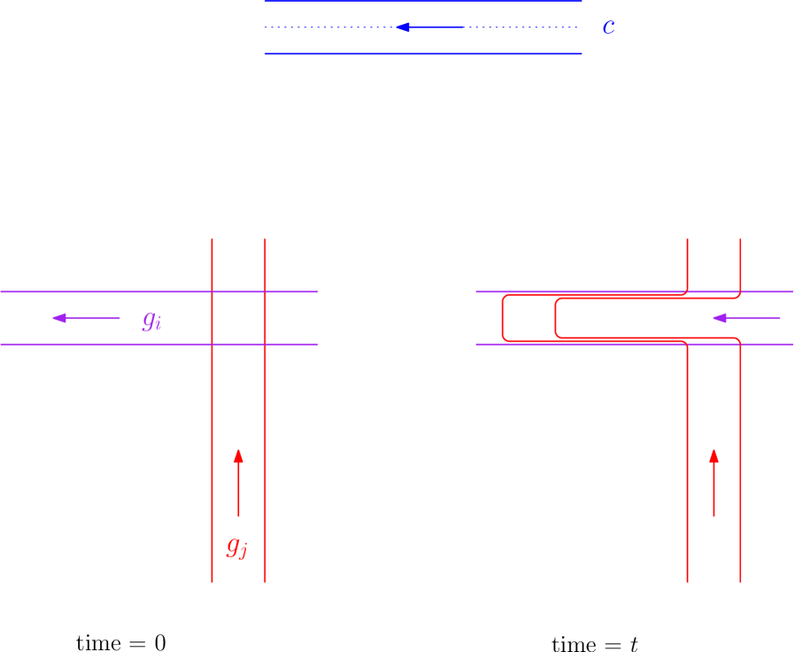
We start with a simple example which will be extended to the general case later. Let $M$ be a closed surface of genus two equipped with a symplectic form $\omega$. Denote by $a,b,a^{\prime},b^{\prime}$ the standard generators of $\pi_{1}(M,*)$ and pick a quasimorphism $r:\pi_{1}(M,*)\to\mathbb{R}$ such that $r(a)=r(b)=0,r(aba^{-1}b^{-1})=1$ (for example, a word counting quasimorphism). Let $\rho:Ham(M)\to\mathbb{R}$ be the quasimorphism induced by $r$. Denote by $P$ a pair of pants whose boundary components represent the free homotopy classes of $aba^{-1}b^{-1},a,a^{-1}$.

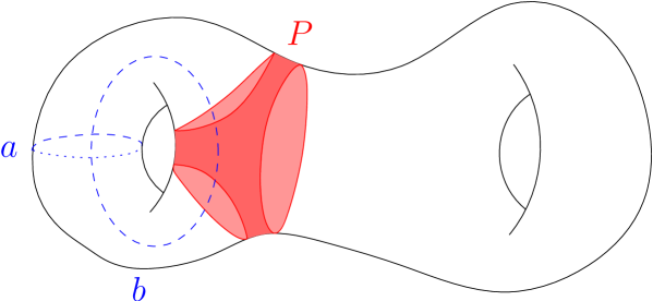
We construct a Hamiltonian $H$ from the indicator function of $P$ which is cut off near the boundary. Note that the flow $\phi_{H}^{t}$ generated by $H$ is controlled by the cutoff and is supported in a tubular neighborhood of the boundary $\partial P$. For a reasonable choice of the cutoff (when the level sets $\{H^{-1}(c)\}_{c\in(0,1)}$ have exactly one connected component near each connected component of $\partial P$) support of the flow consists of three strips around $\partial P$. These strips are foliated by periodic trajectories in the free homotopy classes of $a,a^{-1},aba^{-1}b^{-1}$. The classes $a,a^{-1}$ do not affect the value of $\rho(\phi_{H}^{t})$ and contribution comes only from trajectories in the class $aba^{-1}b^{-1}$. A simple computation shows that $\rho(\phi_{H}^{t})=t$ and it is independent of the cutoff. (Intuitively, when one applies a steeper cutoff, velocity of the flow increases linearly with the slope and inversely proportional to its area of support, so faster rotation is compensated by the reduced volume of motion.)

We adjust the cutoff so that nearly all non-stationary points near $\partial P$ have a fixed rational period. Pick an area preserving parametrization $S^{1}\times(-\varepsilon,\varepsilon)$ with coordinates $(\theta,h)$ near each connected component of $\partial P$ (in our notation $S^{1}=\mathbb{R}/\mathbb{Z}$). Suppose that $P$ is defined in these coordinates by $\{h\geq 0\}$. Pick a natural number $n>1/\varepsilon$ and a smoothing parameter $\delta<<1/n$, define the cutoff function $c:(-\varepsilon,\varepsilon)\to[0,1]$ by

and interpolate it smoothly in the intervals $\left\{0\leq h\leq\delta\right\},\left\{\frac{1}{n}-\delta\leq h\leq\frac{1}{n}\right\}$. Let $H(\theta,h)=c(h)$. As the result, all points in the annulus $\left\{\delta\leq h\leq\frac{1}{n}-\delta\right\}$ have rational period $T=1/n$ and the remaining non-stationary points in $P$ are contained in a region of area $6\delta$ and have controlled dynamics in a sense that their period is at least $1/n$. Note that the smoothing parameter $\delta$ can be chosen arbitrarily small and can be reduced independently of $P$ and $n$. Such adjustment of $\delta$ does not increase the maximal velocity of the flow.

Step I: Given $N>>1$ consider a pair of pants $P$ as above with $\operatorname{Area}(P)<<\frac{1}{N^{2}}$. We place $N$ deformed copies $P_{1}=h_{1}(P),\ldots,P_{N}=h_{N}(P)$ of $P$ (where the deformations $h_{i}$ are symplectic near $P$ and isotopic to the identity) in a way so that no triple intersections of $P_{i}$ occur.

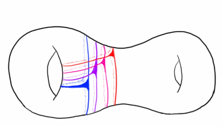
Pick a Hamiltonian function $H$ supported in $P$ as described above. The cutoff of $H$ is adjusted in a way that most (up to a region of area $6\delta<<\operatorname{Area}(P)$) non-stationary points have the same period $T=1/n$ for some $n\in\mathbb{N}$. Denote the resulting Hamiltonian by $H_{P}$ and let $H_{i}$ be the deformations of $H_{P}$ supported in each $P_{i}$ defined by $h_{i}^{*}(H_{i})=H_{P}$. Let $\phi_{i}^{t}=h_{i,*}\phi^{t}_{H_{P}}$ denote their Hamiltonian flows.

Step II: Pick a system of disjoint open neighborhoods $\left\{U_{ij}\right\}_{1\leq i<j\leq N}$ such that $P_{i}\cap P_{j}\subset U_{ij}$. For $i>j$ let $U_{ij}=U_{ji}$. We assume that in each connected component $Q$ of $U_{ij}$ there is enough “empty space” not occupied by $P_{i}$ and $P_{j}$: $\operatorname{Area}(Q)>3\operatorname{Area}((P_{i}\cup P_{j})\cap Q)$. Otherwise we may either repeat the construction applying the same deformations $h_{i}$ to a narrower pair of pants $P$ or deform the symplectic form $\omega$ in the complement of the union of all pairs of pants and redistribute area to satisfy this condition.

Let $t_{0}$ be the minimal time required for any of the flows $\phi_{i}$ to travel between two neighborhoods $U_{kl}$ and $U_{k^{\prime}l^{\prime}}$. Namely, given $t<t_{0}$, $\phi_{i}^{t}(U_{kl})\cap U_{k^{\prime}l^{\prime}}=\emptyset$ for all $\{k,l\}\neq\{k^{\prime},l^{\prime}\}$ and all $1\leq i\leq N$. Pick a natural $m$ such that $\tau:=\frac{T}{m}=\frac{1}{mn}<\frac{t_{0}}{2}$.

Step III: We make a series of adjustments to this construction. The goal is to ensure that most points are $T$-periodic while the rest (that are beyond our direct control) will not travel too far, hence their contribution to the quasimorphism will be small.

First of all, we modify the smoothing parameter $\delta$ that appears in the construction of $H_{P}$. Fix an auxiliary Riemannian metric on $M$. Let $v$ be the maximal point velocity of the flows $\phi_{i}$ and $d_{Q}$ be the maximal diameter of connected components $Q$ of the neighborhoods $U_{ij}$. Let

be a set of homotopy classes of short loops and $r_{\tau}=\max\{r(c)\,\big{|}\,c\in S_{\tau}\}$ be the maximal value of the quasimorphism $r:\pi_{1}(M,*)\to\mathbb{R}$ restricted to $S_{\tau}$. (Short loops represent a finite number of homotopy classes so the maximum is attained.) We pick

where $D$ is the defect of $r$. $H_{i}$ and the deformed flows $\phi_{i}$ are adjusted according to this value of the smoothing parameter $\delta$. Note that this modification does not increase the maximal velocity of the flow. Hence $\tau$ is still less than the travel time between different neighborhoods $U_{kl}$.

Furthermore, perturb $P_{1},\ldots,P_{N}$ inside the neighborhoods $U_{ij}$ so that

We apply the same perturbations to the Hamiltonian functions $H_{i}$ and the flows $\phi_{i}$. This modification does not affect dynamics of the flows outside the neighborhoods $U_{ij}$, hence the minimal travel time between neighborhoods is still greater than $\tau$. Moreover, the modified flows may have increased velocities locally inside $U_{ij}$, but on a larger scale (time $\tau$ and above) they travel approximately the same distance.

Let $\Phi^{t}=\phi_{1}^{t}\circ\ldots\circ\phi_{N}^{t}$ be the composition of the time-$t$ maps of the flows. We claim that for $t=\tau$,

while the Hofer norm is bounded by $2\tau$. Taking $N\to\infty$, we deduce that $\rho$ is not Lipschitz.

By the composition formula, the flow $\Phi^{t}$ is generated by the time-dependent Hamiltonian

Namely, the pairs of pants $P_{i}$ which support the Hamiltonian functions $H_{i}$ are deformed and “dragged” along the flows. For time $t<t_{0}$ supports of the summands cannot have triple intersections: that happens only after some $P_{i}$ is dragged by $\phi_{j}^{t}$ to a point where it intersects some (possibly deformed) $P_{k}$. That means that certain points $p\in U_{ij}$ have arrived in (or passed through) other neighborhood $U_{jk}$ and that cannot happen before $t=t_{0}$. As each summand admits values in the interval $[0,1]$, $\max G_{t}-\min G_{t}\leq 2$ for all $0\leq t<t_{0}$ and the bound on the Hofer norm follows.

We estimate the value of the quasimorphism $\rho(\Phi^{\tau})$. Intuitively speaking, the time-$\tau$ maps $\{\phi_{i}^{\tau}\}$ “almost commute” (commute in the complement of a subset of area $7N\delta$), hence their contribution to the quasimorphism “almost adds up” (up to a defect which is small compared to the values $\rho(\phi_{i}^{\tau})$ and is controlled by $\delta$).

Pick $k\leq N$. We consider three $\phi_{k}^{\tau}$-invariant regions in $M$ according to the dynamics of points under $\phi_{k}^{\tau}$:

1. (1)

   points outside $P_{k}$ and those points inside that are stationary under $\phi_{k}$. They do not contribute to $\rho(\phi_{k}^{\tau})$.

2. (2)

   the set $A_{k}$ of $m$-periodic points under $\phi_{k}^{\tau}$ that never hit any of the remaining pairs of pants $\{P_{i}\}_{i\neq k}$.

   All non-stationary points are contained in the three cutoff strips near $\partial P_{k}$. Each strip has area $\frac{1}{n}$ and we have to remove those points that are not $m$-periodic due to smoothing. Thus the set of $m$-periodic points has area bounded between $\frac{3}{n}-6\delta$ and $\frac{3}{n}$. After removing points whose trajectories intersect $\{P_{i}\}_{i\neq k}$ we get the estimate

   $$\operatorname{Area}(A_{k})\geq\frac{3}{n}-6\delta-m\sum_{i\neq k}\operatorname{Area}(P_{i}\cap P_{k})\geq\frac{3}{n}-6\delta-mN\cdot\frac{\delta}{mN}=\frac{3}{n}-7\delta$$

   Points of $A_{k}$ are distributed in three strips near $\partial P_{k}$ and their trajectories, depending on the strip, represent either $a,a^{-1}$ or $aba^{-1}b^{-1}$. $a$ and $a^{-1}$ do not affect $\rho(\phi_{k}^{\tau})$ while the set $A^{\prime}_{k}$ of points in the class $aba^{-1}b^{-1}$ has $\operatorname{Area}(A^{\prime}_{k})\geq\frac{1}{n}-3\delta$ and contributes

   $$\frac{\operatorname{Area}(A^{\prime}_{k})\cdot r(aba^{-1}b^{-1})}{m}\geq\frac{1}{nm}-\frac{3\delta}{m}=\tau-\frac{3\delta}{m}$$

3. (3)

   the set $B_{k}$ containing the rest of points (non-stationary points whose period is different from $m$ or whose trajectory under $\phi_{k}^{\tau}$ hits other pairs of pants). By a similar computation, $\operatorname{Area}(B_{k})\leq 7\delta$. While we have less control on the dynamics of $B_{k}$, we note that the velocity of points in $B_{k}$ under the flow $\phi_{k}$ is bounded by $v$ outside neighborhoods $Q$ of the intersections $P_{k}\cap P_{j}$ (it can still be very large inside $Q$ because of the adjustments). Also note that the time needed to travel between different neighborhoods is larger than $\tau$. Hence for each $p\in B_{k}$, the trajectory $\{\phi_{k}^{t}(p))\}_{t\in[0,\tau]}$ has length at most $\tau v+d_{Q}$.

   Applying stabilization, the trajectory of $p$ under $(\phi_{k}^{\tau})^{K}$ has length bounded by $K(\tau v+d_{Q})$ and $\left[l_{p}\left((\phi_{k}^{\tau})^{K}\right)\right]$ can be presented as a product of at most $K$ elements from $S_{\tau}$, so $r([l_{p}((\phi_{k}^{\tau})^{K})])\leq K(r_{\tau}+D)$. The contribution of $B_{k}$ to $\rho(\phi_{k}^{\tau})$ is bounded in the absolute value by

   $$\lim_{K\to\infty}\frac{1}{K}\int_{B_{k}}|r([l_{p}((\phi_{k}^{\tau})^{K})])|\omega\leq(r_{\tau}+D)\cdot\operatorname{Area}(B_{k})=7\delta(r_{\tau}+D).$$

Now note that for all $k\leq N$, $A_{k}$ is $\Phi^{\tau}$-invariant and the action of $\Phi^{\tau}$ coincides with that of $\phi_{k}^{\tau}$. Indeed, for a point $p\in A_{k}$, $(\Phi^{\tau})^{K}(p)=(\phi_{k}^{\tau})^{K}(p)$ for all $K$ as $p$ never hits the pairs of pants $\{P_{i}\}_{i\neq k}$. More than that, the trajectory $\{\Phi^{t}(p)\}_{t\in[0,\tau]}$ is homotopic relative endpoints to $\{\phi_{k}^{t}(p)\}_{t\in[0,\tau]}$ (other ingredients of $\Phi^{t}(p)=\phi_{1}^{t}\circ\ldots\circ\phi_{N}^{t}(p)$ can be homotoped away). The same is true for iterations of $\Phi^{\tau}$, hence $A_{k}$ contributes to $\rho(\Phi^{\tau})$ the same amount as to $\rho(\phi_{k}^{\tau})$. We finish with an observation that the sets $\{A_{k}\}_{k=1}^{N}$ are disjoint and do not intersect $B=\bigcup_{j=1}^{N}B_{j}$.

Let $p\in B$. If $p\in P_{N}$, the trajectory $\{\Phi^{t}(p)\}_{t\in[0,\tau]}$ is the trajectory $\{\phi_{N}^{t}(p)\}_{t\in[0,\tau]}$ which was possibly deformed by the flows $\phi_{N-1},\ldots,\phi_{1}$. Such deformation occurs each time $\{\phi_{N}^{t}(p)\}_{t\in[0,\tau]}$ crosses a pair of pants $P_{N-1},\ldots,P_{1}$. Within time $\tau$ only one such crossing is possible. As the result, $\{\Phi^{t}(p)\}_{t\in[0,\tau]}$ is homotopic (relative endpoints) to a path of length at most $(2\tau v+d_{Q})$ (the path can be longer than $\tau v+d_{Q}$ when $\{\phi_{N}^{t}(p)\}_{t\in[0,\tau]}$ either starts or ends at the intersection with other pair of pants). The same argument can be applied to points $p\in B\cap(P_{N-1}\setminus P_{N})$, $p\in B\cap(P_{N-2}\setminus(P_{N}\cup P_{N-1}))$ and so on by induction. After taking $K$ iterations, trajectory of any $p\in B$ is homotopic relative endpoints to a path shorter than $2K(\tau v+d_{Q})$, thus the contribution of $B$ to $\rho(\Phi^{\tau})$ in the absolute value is at most

As a summary, points from $A=\bigcup_{i=1}^{N}A_{i}$ contribute to $\rho(\Phi^{\tau})$ at least $N\tau-\frac{3N\delta}{m}$. $B=\bigcup_{i=1}^{N}B_{i}$ alters the result by at most $14N\delta(r_{\tau}+D)$. Points $p\in M\setminus(A\cup B)$ are stationary and do not contribute. We deduce

Let $M$ be a symplectic surface of finite type and suppose $r:\pi_{1}(M,*)\to\mathbb{R}$ is a genuine homogeneous quasimorphism. Pick $a,b\in\pi_{1}(M,*)$ such that $r(ab)\neq r(a)+r(b)$ (without loss of generality assume that $d_{r}=r(a)+r(b)-r(ab)>0$). Let $\alpha,\beta$ be based loops representing $a,b$, respectively. Denote by $\rho$ be the induced quasimorphism on $Ham(M)$. Let $\gamma=\alpha*\beta$. We wish to construct a Hamiltonian diffeomorphism $\Phi^{\tau}$ such that $\rho(\Phi^{\tau})>>\|\Phi^{\tau}\|_{H}$.

Step I: Pick a small tubular neighborhood $P$ of $\gamma$. Applying $C^{0}$-small perturbations to $\alpha,\beta,\gamma$ we may assume that the three curves intersect (and self-intersect) transversely in a finite number of points and still lie in $P$.

Step II: Consider $N$ deformed copies ($N>>1$) $P_{1}=h_{1}(P),\ldots,P_{N}=h_{N}(P)$ of $P$ where the deformations $h_{i}$ are isotopic to the identity and area-preserving near $P$ so that:

• •

  no triple intersections of $\{P_{i}\}_{i=1}^{N}$ occur

• •

  the collection of loops $Q=\{\alpha_{i}=h_{i}(\alpha)\}_{i}\cup\{\beta_{i}=h_{i}(\beta)\}_{i}\cup\{\gamma_{i}=h_{i}(\gamma)\}_{i}$ does not have triple intersection/self-intersection points, the total number of intersections is finite and they are all transverse.

Step III: Construct a time-dependent Hamiltonian flow $\Phi^{t}$ supported in a narrow tubular neighborhood of curves from $Q$ which translates points along $\{\alpha_{i}\}_{i=1}^{N},\{\beta_{i}\}_{i=1}^{N}$ preserving orientation of curves and along $\{\gamma_{i}\}_{i=1}^{N}$ with reversed orientation.

Local picture:

• •

  near a curve $c\in Q$ and away from intersection points the flow is a parallel translation of a narrow strip around $c$ with fixed velocity and flux $1$. The flow is cut off in a smooth way so that it remains parallel to $c$ and the area affected by the cutoff is small.

• •

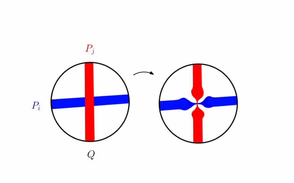
  near an intersection of two curves $c_{i},c_{j}$ (or a self-intersection of two arcs $c_{i},c_{j}$ of the same curve from $Q$): construct the flows $g_{i},g_{j}$ parallel to $c_{i},c_{j}$ as in the previous case. We may symplectically perturb $g_{i},g_{j}$ near $c_{i}\cap c_{j}$ to ensure that $\operatorname{Area}(\operatorname{supp}(g_{i})\cap\operatorname{supp}(g_{j}))$ is sufficiently small. Define the local flow $\Phi^{t}$ to be the composition $g_{i}^{t}\circ g_{j}^{t}$. Intuitively speaking, the curve $c_{j}$ and the flow $g_{j}$ following $c_{j}$ “drift” with $g_{i}^{t}$.

For $t$ small enough the flow charts can be adjusted and patched together to form a global symplectic time-dependent flow $\Phi^{t}$. More than that, using local adjustments, one can ensure that:

• •

  flow strips around $\alpha_{i},\beta_{i},\gamma_{i}$ are narrow enough and stay inside $P_{i}$.

• •

  local velocities are chosen in a way so that if one ignores all intersections, time $T$ needed to traverse a loop $c\in Q$ is the same for all loops in $Q$.

• •

  the total area of the cutoff zones and intersections / self-intersections of the flow strips is at most $\delta$ ($\delta$ is a small parameter which will be specified later).

The construction described above works for $t\leq t_{0}$ where $t_{0}$ is the minimal time needed for an intersection point $p\in c_{i}\cap c_{j}$ to leave the appropriate chart when it follows the flows $g_{i}$ or $g_{j}$.

Clearly, the flow $\Phi^{t}$ is area-preserving. We claim that it has zero flux, hence is Hamiltonian. Indeed, the flux along each $\alpha_{i},\beta_{i}$ is $1$ while the flux along $\gamma_{i}$ is $-1$ due to reversed orientation. A generic cycle $c$ in $(M,\partial M)$ satisfies $\#c\cap\alpha_{i}+\#c\cap\beta_{i}=\#c\cap\gamma_{i}$ (the intersection points are counted with signs), so the fluxes cancel out. Denote by $H_{t}$ the Hamiltonian function which generates $\Phi^{t}$. It is a well known fact that $H_{t}(p)-H_{t}(q)$ equals the flux of $\Phi^{t}$ through a curve which connects $p$ to $q$ (for a Hamiltonian flow the flux depends on the endpoints and not on the curve itself). The argument above also shows that the flux between two points $p,q\notin\bigcup P_{i}$ is zero, hence, up to a shift by appropriate constant, $\operatorname{supp}H_{t}\subseteq\bigcup P_{i}$.

For a generic curve $c$ connecting two points $p,q\in P_{1}\setminus(\alpha_{1}\cup\beta_{1}\cup\gamma_{1})$ let $K_{c}=\#c\cap\alpha_{1}+\#c\cap\beta_{1}-\#c\cap\gamma_{1}$ (count with signs). Roughly, if one ignores the width of flow strips around the curves, $K_{c}$ measures the flux between $p$ and $q$ of the flows along $\alpha_{1},\beta_{1},\gamma_{1}$. $K=\max_{c}K_{c}$ equals the maximal flux between any two points in $P_{1}$. Fluxes of flows inside each $P_{i}$ are additive, so as long as no triple intersections are allowed and $t\leq t_{0}$ (meaning the curves do not drift far and combinatorics of their intersections does not change), the maximal flux of $\Phi^{t}$ (and hence the variation of $H_{t}$) is at most $2K$. That is, the Hofer length of the isotopy $\Phi^{t}$ is bounded by $2Kt$. Note that the bound $K$ may depend on the perturbations performed in Step I but does not depend on the choice of $N$ in Step II.

Pick $\tau=\frac{T}{m}\leq t_{0}$ for some $m\in\mathbb{N}$. The flow strip around a curve $c\in Q$ has flux $1$ and period $T$, hence has area equal to $T$ (up to effects of smoothing which slow down the flow and are controlled by $\delta$). We subtract points which are slowed by smoothing and also those whose trajectory under $\{(\Phi^{\tau})^{k}\}_{k\in\mathbb{Z}}$ lands on the intersections/self-intersections of strips. The remaining region of area $T-O(\delta)$ is $m$-periodic and contributes to $\rho(\Phi^{\tau})$ either

in the case $c=\alpha_{i}$, $\tau r(b)+O(\delta)$ if $c=\beta_{i}$ or $-\tau r(ab)+O(\delta)$ when $c=\gamma_{i}$ for some $i\leq N$.

The rest of non-stationary points (either affected by smoothing or those visiting intersections of strips) are contained in a region $B$ of area $O(\delta)$. The long-term dynamics of $p\in B$ can be complicated, but locally (till time $\tau$) $p$ can visit at most one intersection of strips, so the length of trajectory $\{\Phi^{t}(p)\}_{t\in[0,\tau]}$ is uniformly bounded. As the result, $\left|\frac{1}{k}r([l_{p}((\Phi^{\tau})^{k})])\right|$ is also uniformly bounded by some $C>0$ and the contribution of $B$ to $\rho(\Phi^{\tau})$ is bounded in the absolute value by

Summing up,

Now we pick $\delta=\delta(N)$ small enough to ensure $\rho(\Phi^{\tau})>\tau(N-1)d_{r}$ and perform rearrangements of smoothing and intersection zones to comply with this chosen value of $\delta$. These local adjustments do not affect $t_{0}$ or estimates of trajectory lengths, hence all computations we performed above remain in place. The claim follows by picking $N$ such that $Nd_{r}>>2K$.

The construction above can be lifted to a symplectic ball bundle $\widehat{M}\to M$. We lift the flow $\Phi^{t}$ from $M$ and cut it off near $\partial\widehat{M}$. When the cutoff is steep enough, it affects only a small volume of motion while keeping dynamics under control (cutoff keeps the $M$ component of the flow velocity bounded and introduces a fast rotation around the boundary in the fiber coordinates. This rotation does not affect average homotopy classes of orbits.) Hence its effect on the quasimorphism $\widehat{\rho}:Ham(\widehat{M})\to\mathbb{R}$ can be made arbitrarily small. The bounds on the Hofer length in $\widehat{M}$ remain the same as in $M$ and non-continuity follows.

Let $M$ be a higher dimension symplectic manifold, $r:\pi(M,*)\to\mathbb{R}$ a genuine homogeneous quasimorphism. Let $\alpha,\beta$ be based loops in $M$ such that $r([\alpha*\beta])\neq r([\alpha])+r([\beta])$. Perturb $\alpha,\beta$ so that they intersect at one point and that near the intersection they lie in a symplectic $2$-disk $D$. $D$ can be extended to a smooth symplectic surface $\Sigma$ with boundary which contains both $\alpha$ and $\beta$. By the symplectic neighborhood theorem, a small neighborhood of $\Sigma$ in $M$ is symplectomorphic to a ball bundle over $\Sigma$. Now we may apply the construction for ball bundles and show non-continuity of the quasimorphism induced by $r$.

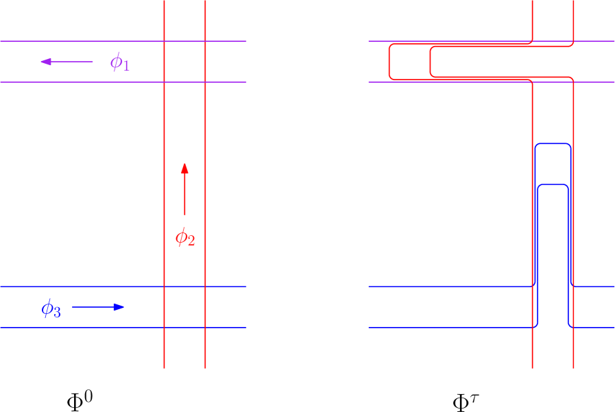
Let $(M,\omega)$ be a symplectic surface of finite type and area $1$, equipped with an auxiliary Riemannian metric. Denote by $B_{k}$ the braid group with $k$ strands in $M$ and by $PB_{k}$ the pure braid group. Suppose $\{g_{t}\}\in Ham(M)$ is an isotopy starting at the identity and ending at $g$. Pick $k$ distinct points $w_{1},\ldots,w_{k}$ in $M$ to be a basepoint $\mathbf{w}$ in the configuration space $X_{k}(M)$. For an $\mathbf{x}=(x_{1},\ldots,x_{k})\in X_{k}(M)$ we construct $k$ based loops $l_{w_{j},x_{j}}(g_{t})$ by concatenating a short geodesic path $\gamma_{w_{j},x_{j}}$ with the trajectory $\{g_{t}(x_{j})\}$ and closing the loop by a short geodesic path $\gamma_{g(x_{j}),w_{j}}$. For almost all $\mathbf{x}\in X_{k}$, the $k$-tuple of loops $l_{\mathbf{x}}(g_{t})=\left(l_{w_{1},x_{1}}(g_{t}),\ldots,l_{w_{k},x_{k}}(g_{t})\right)$ defines a based loop in $X_{k}(M)$. $\pi_{1}(X_{k},\mathbf{w})$ can be identified with the pure braid group $PB_{k}$, hence $[l_{\mathbf{x}}(g_{t})]$ defines an element in $PB_{k}$.

Let $r:B_{k}\to\mathbb{R}$ be a homogeneous quasimorphism. Then

defines a quasimorphism $\hat{\rho}:\widetilde{Ham(M)}\to\mathbb{R}$ and its homogenization

does not depend on the choices of metric, basepoint $\mathbf{w}$, geodesic paths or $g_{t}$, resulting in a homogeneous quasimorphism $\rho:Ham(M)\to\mathbb{R}$. For a more detailed explanation see  [Bra].

This construction generalizes the quasimorphisms by Polterovich: $PB_{1}(M)\simeq\pi_{1}(M,*)$, therefore for $k=1$ both constructions agree.

References

- [Ban] A. Banyaga. Sur la structure du groupe des diffeomorphismes qui preservent une forme symplectique. Comm.Math.Hel, 53:174–227, 1978.
- [BEP] P. Biran, M. Entov, and L. Polterovich. Calabi quasimorphisms for the symplectic ball. Commun. Contemp. Math., 6(5):793–802, 2004.
- [Bir] Joan S. Birman. Braids, Links, and Mapping Class Groups. (AM-82). Princeton University Press, 1974.
- [BO] L. Buhovsky and Y. Ostrover. On the uniqueness of Hofer’s geometry. Geom. Funct. Anal., 21(6):1296–1330, 2011.
- [Bra] M. Brandenbursky. Bi-invariant metrics and quasi-morphisms on groups of Hamiltonian diffeomorphisms of surfaces. Int. J. of Math., 26(9), 2013.
- [BS1] Michael Brandenbursky and Egor Shelukhin. On the large-scale geometry of the -metric on the symplectomorphism group of the two-sphere. arXiv e-prints, page arXiv:1304.7037, Apr 2013.
- [BS2] Michael Brandenbursky and Egor Shelukhin. On the -geometry of autonomous Hamiltonian diffeomorphisms of surfaces. Mathematical Research Letters, 22, 05 2014.
- [BS3] Michael Brandenbursky and Egor Shelukhin. The -diameter of the group of area-preserving diffeomorphisms of . Geom. Topol., 21(6):3785–3810, 2017.
- [Buh] L. Buhovsky. Private communication, December 2018.
- [Cal] Danny Calegari. scl., volume 20. Tokyo: Mathematical Society of Japan, 2009.
- [EP] M. Entov and L. Polterovich. Calabi quasimorphism and quantum homology. Int. Math. Res. Not., 2003(30):1635–1676, 2003.
- [Fat] Albert Fathi. Transformations et homeomorphismes preservant la mesure : systemes dynamiques minimaux. PhD thesis, Universite Paris-Sud, 1980.
- [GtG] Jean-Marc Gambaudo and Étetienne Ghys. Enlacements asymptotiques. Topology, 36(6):1355 – 1379, 1997.
- [Hof] H. Hofer. On the topological properties of symplectic maps. Proc. Royal Soc. Edinburgh, 115(1-2):25–38, 1990.
- [Ish] Tomohiko Ishida. Quasi-morphisms on the group of area-preserving diffeomorphisms of the 2-disk via braid groups. Proceedings of the American Mathematical Society, Series B, 1, 04 2012.
- [Kha] M. Khanevsky. Hofer’s metric on the space of diameters. JTA, 1(4):407–416, 2009.
- [Pol] L. Polterovich. Floer homology, dynamics and groups. In Morse Theoretic Methods in Nonlinear Analysis and in Symplectic Topology, volume 217 of NATO Sci. Ser. II: Math, Phys and Chem, pages 417–438. Springer Netherlands, 2006.
- [Sey] Sobhan Seyfaddini. Unboundedness of the Lagrangian Hofer distance in the Euclidean ball. Electronic Research Announcements in Mathematical Sciences [electronic only], 21:1–7, 10 2013.