Quasistatic evolution and accretive phase-change
in finite-strain viscoelastic solids

Andrea Chiesa University of Vienna, Faculty of Mathematics and Vienna School of Mathematics, Oskar-Morgenstern-Platz 1, A-1090 Vienna, Austria andrea.chiesa@univie.ac.at http://www.mat.univie.ac.at/

\sim

achiesa and Ulisse Stefanelli University of Vienna, Faculty of Mathematics, Oskar-Morgenstern-Platz 1, A-1090 Vienna, Austria, University of Vienna, Vienna Research Platform on Accelerating Photoreaction Discovery, Währingerstraße 17, 1090 Wien, Austria, and Istituto di Matematica Applicata e Tecnologie Informatiche E. Magenes, via Ferrata 1, I-27100 Pavia, Italy ulisse.stefanelli@univie.ac.at http://www.mat.univie.ac.at/

\sim

stefanelli

Abstract.

We investigate the quasistatic evolution problem for a two-phase viscoelastic material at finite strains. Phase evolution is assumed to be irreversible as one phase accretes in time in its normal direction, at the expense of the other. Mechanical response depends on the phase, and growth is influenced by the mechanical state at the boundary of the accreting phase, making the model to be fully coupled. This setting is inspired by the early stage development of solid tumors, as well as by the swelling of polymer gels. We formulate the evolution problem by coupling the quasistatic balance of momenta in weak form and the growth dynamics in the viscosity sense. Both a diffused- and a sharp-interface variant of the model are proved to admit solutions.

Key words and phrases:

Accretive growth, viscoelastic solid, finite-strain, quasistatic evolution, variational formulation, viscosity solution, existence.

2020 Mathematics Subject Classification:

74F99, 74G22, 49L25

1. Introduction

This paper is concerned with the quasistatic evolution of a viscoelastic compressible solid undergoing a phase transition. We assume that the material presents two phases, of which one grows at the expense of the other by accretion. In particular, the phase-transition font evolves in a normal direction to the accreting phase, with a growing rate depending on the deformation. This behavior is indeed common to different material systems. It may be observed in the early stage development of solid tumors [6, 28, 56], where the neoplastic tissue invades the healthy one. Swelling in polymer gels also follows a similar dynamics, with the swollen phase accreting in the dry one [31, 50] and causing a volume increase. Accretive phase-growth can be observed in some solidification processes [43, 53], as well.

The focus of the modelization is on describing the interplay between mechanical deformation and accretion, On the one hand, the two phases are assumed to have a different mechanical response, having an effect on the viscoelastic evolution of the medium. On the other hand, the time-dependent mechanical deformation is assumed to influence the growth process, as is indeed common in biomaterials [21], polymeric gels [57], and solidification [44]. The mechanical and phase evolutions are thus fully coupled.

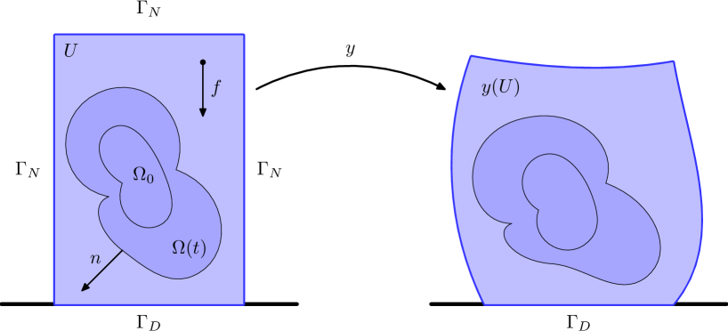
The state of the system is described by the pair $(y,\theta):[0,T]\times U\to\mathbb{R}^{d}\times[0,\infty)$ , where $T>0$ is some final time and $U$ is the reference configuration of the body. Here, $y$ is the deformation of the medium while $\theta$ determines its phase. More precisely, for all $t\in[0,T]$ the accreting (growing) phase is identified as the sublevel $\Omega(t):=\{x\in U\ |\ \theta(x)<t\}$ , whereas the receding phase corresponds to $U\setminus\overline{\Omega(t)}$ . The value $\theta(x)$ formally corresponds to the time at which the point $x\in U$ is added to the growing phase. As such, $\theta$ is usually referred to as time-of-attachment function. An illustration of the mechanical setting is given in Figure 1.

Refer to caption — Figure 1. Setting of the model in the sharp-interface case.

As growth processes and mechanical equilibration typically occur on very different time scales, we assume that the body is in quasistatic equilibrium. This calls for specifying the stored energy density $W(\theta(x){-}t,\nabla y)$ and the viscosity $R(\theta(x){-}t,\nabla y,\nabla\dot{y})$ of the medium, as well as the applied body forces $f(\theta(x){-}t,x)$ . All these quantities are assumed to be dependent on the phase via the sign of $\theta(x){-}t$ , which indeed distinguishes the two phases, in the spirit of the celebrated level-set method [40, 45]. In addition, we include a second-gradient regularization term in the energy of the form $H(\nabla^{2}y)$ , which we take to be phase independent, for simplicity. All in all, the quasistatic equilibrium system takes the form

{}-\operatorname{div}\left(\partial_{\nabla y}W(\theta(x){-}t,\nabla y)+\partial_{\nabla\dot{y}}R(\theta(x){-}t,\nabla y,\nabla\dot{y})-\operatorname{div}{\rm D}H(\nabla^{2}y)\right)=f(\theta(x){-}t,x).

(1.1)

This system is solved weakly, complemented by mixed boundary conditions on $y$ and a homogeneous natural condition on the hyperstress $-\operatorname{div}\,{\rm D}H(\nabla^{2}y)$ , namely,

	$\displaystyle y={\rm id}\ \ \text{on}\ \ [0,T]\times\Gamma_{D},$		(1.2)
	$\displaystyle{\rm D}H(\nabla^{2}y){:}(\nu\otimes\nu)=0\ \ \text{on}\ \ [0,T]\times\partial U,$		(1.3)
	$\displaystyle\left(\partial_{\nabla y}W(\theta(x){-}t,\nabla y){+}\partial_{\nabla\dot{y}}R_{\varepsilon}(\theta(x){-}t,\nabla y,\nabla\dot{y})\right)\nu$
	$\displaystyle\quad-{\rm div}_{S}\,({\rm D}H(\nabla^{2}y))=0\ \ \text{on}\ \ [0,T]\times\Gamma_{N},$		(1.4)

where $\nu$ is the outer unit normal to $\partial U$ , $\Gamma_{D}$ and $\Gamma_{N}$ are the Dirichlet and Neumann part of the boundary $\partial U$ , respectively, and ${\rm div}_{S}$ denotes the surface divergence on $\partial U$ [27].

The quasistatic equilibrium system is coupled to the phase evolution by requiring that the time-of-attachment function $\theta$ solves the generalized eikonal equation

\gamma\big{(}y(\theta(x),x),\nabla y(\theta(x),x)\big{)}|\nabla(-\theta)(x)|=1

(1.5)

for all $x$ in the complement of a given initial set $\Omega_{0}\subset\subset U$ where we set $\theta=0$ . This corresponds to assuming that $\Omega(t)$ accretes in its normal direction, with growth rate $\gamma(\cdot)>0$ . More precisely, the evolution of the generic point $x(t)$ on the boundary $\partial\Omega(t)$ follows the ODE flow

\dot{x}(t)=\gamma\big{(}y(t,x(t)),\nabla y(t,x(t))\big{)}\,n(x(t))

where $n(x(t))$ indicates the normal to $\partial\Omega(t)$ at $x(t)$ . Accretive growth is paramount to a wealth of different biological models [49], including plants and trees [15, 17] and the formation of hard tissues like horns or shells [36, 46, 51]. The dependence of the growth rate $\gamma$ on the actual position and strain is intended to model the possible influence of local features such as nutrient concentrations, as well as of the local mechanical state [21].

Note that accretive growth occurs in a variety of nonbiological systems, as well. These include crystallization [29, 55], sedimentation of rocks [18], glacier formation, accretion of celestial bodies [8], as well as technological applications, from epitaxial deposition [32], to coating, masonry, and 3D printing [20, 30], just to mention a few.

By assuming smoothness and differentiating the equation $\theta(x(t))=t$ in time one obtains $\nabla\theta(x(t)){\cdot}\dot{x}(t)=1$ . This, together with the above flow rule for $x(t)$ and $n(x(t))=\nabla\theta(x(t))/|\nabla\theta(x(t))|$ , originates the generalized eikonal equation (1.5). Note that the growth rate $\gamma$ in (1.5) depends on the actual deformation $y(\theta(x),x)$ and strain $\nabla y(\theta(x),x)$ at the growing interface, making the system (1.1)–(1.5) fully coupled.

We specify the initial conditions for the system by setting

	$\displaystyle\theta=0\ \ \text{on}\ \Omega_{0},$		(1.6)
	$\displaystyle y(0,\cdot)=y_{0}\ \ \text{on}\ U,$		(1.7)

where the initial deformation $y_{0}$ and the initial portion of the growing phase $\Omega_{0}$ are given. Note that $\Omega_{0}$ is not required to be connected, in order to possibly model the onset of the accreting phase at different sites. On the other hand, the evolution described by (1.5) does not preserve the topology and disconnected accreting regions may coalesce over time.

The aim of this paper is to present an existence theory to the initial and boundary value problem (1.1)–(1.7). We tackle both a sharp-interface and a diffused-interface version of the model, by tuning the assumptions on $W$ and $R$ , see Sections 2.3–2.4. More precisely, in the diffused-interface model we assume that energy and dissipation densities change smoothly as functions of the phase indicator $\theta(x){-}t$ across a region of width $\varepsilon>0$ , namely for $-\varepsilon/2<\theta(x)-t<\varepsilon/2$ . On the contrary, in the sharp-interface case material potentials are assumed to be discontinuous across the phase-change surface $\{\theta(x)=t\}$ .

In both regimes, we prove that the fully coupled system (1.1)–(1.7) admits a weak/viscosity solution, see Definition 2.1 below. More precisely, the quasistatic viscous evolution (1.1)–(1.4) is solved weakly, whereas the growth dynamics equation (1.5) is solved in the viscosity sense, see Theorem 2.1. We moreover prove that solutions fulfill the energy equality, where the energetic contribution of the phase transition is characterized, see Proposition 2.1. As a by-product, solutions of the diffused-interface model for $\varepsilon>0$ are proved to converge up to subsequences to solutions of the sharp-interface model as the parameter $\varepsilon$ converges to $0$ , see Corollary 2.1.

Before going on, let us mention that the engineering literature on growth mechanics is vast. Without any claim of completeness, we mention [47, 58] and [33, 37, 38, 48, 52] as examples of linearized and finite-strain theories, respectively. On the other hand, mathematical existence theories in growth mechanics are scant, and we refer to [3, 12, 19] for some recent results. To the best of our knowledge, no existence result for finite-strain accretive-growth mechanics is currently available. In the linearized case, an existence result for the model [58] has been obtained in [13].

The paper is structured as follows. Section 2 is devoted to the statement of the main existence result, Theorem 2.1. In section 3, we give the proof of the energy identity. The proof of Theorem 2.1 is then split in Sections 4 and 5, respectively focusing on the diffused-interface and the sharp-interface setting. In the diffused-interface case, the proof relies on an iterative construction, where the mechanical and the growth problems are solved in alternation. The existence proof for the sharp-interface model is obtained by passing to the limit as $\varepsilon\to 0$ .

2. Main results

In this section, we specify assumptions, introduce the weak/viscosity notion of solution, and state the main results for problem (1.1)–(1.7).

2.1. Notation

In what follows, we denote by $\mathbb{R}^{d\times d}$ the Euclidean space of $d{\times}d$ real matrices, $d\geq 2$ , by $\mathbb{R}^{d\times d}_{\rm sym}$ the subspace of symmetric matrices, and by $I$ the identity matrix. Given $A\in\mathbb{R}^{d\times d}$ , we indicate its transpose by $A^{\top}$ and its Frobenius norm by $|A|^{2}:=A{:}A$ , where the contraction product between matrices $A,\,B\in\mathbb{R}^{d\times d}$ is defined as $A{:}B:=A_{ij}B_{ij}$ (we use the summation convention over repeated indices). Analogously, let $\mathbb{R}^{d\times d\times d}$ be the set of real $3$ -tensors, and define their contraction product as $A\smash{\vdots}B:=A_{ijk}B_{ijk}$ for $A,B\in\mathbb{R}^{d\times d\times d}$ . Moreover, given a symmetric positive definite 4-tensor $\mathbb{C}\in\mathbb{R}^{d\times d\times d\times d}$ and the matrix $A\in\mathbb{R}^{d\times d}$ we indicate by $\mathbb{C}{:}A\in\mathbb{R}^{d\times d}$ and $A{:}\mathbb{C}\in\mathbb{R}^{d\times d}$ the matrices given in components by $(\mathbb{C}{:}A)_{ij}=\mathbb{C}_{ijk\ell}A_{k\ell}$ and $(A{:}\mathbb{C})_{ij}=A_{k\ell}C_{k\ell ij}$ , respectively. We shall use the following matrix sets

	$\displaystyle{\rm SL}(d):=\{A\in\mathbb{R}^{d\times d}\;\|\;\det A=1\},$
	$\displaystyle{\rm SO}(d):=\{A\in{\rm SL}(d)\;\|\;AA^{\top}=I\},$
	$\displaystyle{\rm GL}_{+}(d):=\{A\in\mathbb{R}^{d\times d}\;\|\;\det A>0\}.$

The scalar product of two vectors $a,\,b\in\mathbb{R}^{d}$ is classically indicated by $a{\cdot}b$ . The symbol $B_{R}\subset\mathbb{R}^{d}$ denotes the open ball of radius $R>0$ and center $0\in\mathbb{R}^{d}$ , $|E|$ indicates the Lebesgue measure of the Lebesgue-measurable set $E\subset\mathbb{R}^{d}$ , and $\mathbbm{1}_{E}$ is the corresponding characteristic function, namely, $\mathbbm{1}_{E}(x)=1$ for $x\in E$ and $\mathbbm{1}_{E}(x)=0$ otherwise. For $E\subset\mathbb{R}^{d}$ nonempty and $x\in\mathbb{R}^{d}$ we define ${\rm dist}(x,E):=\inf_{e\in E}|x{-}e|$ . We denote by $\mathcal{H}^{d-1}$ the $(d{-}1)$ -dimensional Hausdorff measure.

In the following, we indicate by $c$ a generic positive constant, possibly depending on data but independent of $\varepsilon$ and of the discretization step $\tau$ . Note that the value of $c$ may change from line to line.

2.2. Admissible deformations

Fix the final time $T>0$ and let the reference configuration $U\subset\mathbb{R}^{d}$ be nonempty, open, connected, and bounded. We assume that the boundary $\partial U$ is Lipschitz, with $\Gamma_{D},\,\Gamma_{N}\subset\partial U$ disjoint and open in the topology of $\partial U$ , $\Gamma_{D}\not=\emptyset$ and $\overline{\Gamma_{D}}\cap\overline{\Gamma_{N}}=\partial U$ , where the closure is taken in the topology of $\partial U$ . In the following, we use the short-hand notation $Q:=(0,T)\times U$ and $\Sigma_{D}:=(0,T)\times\Gamma_{D}$ .

Deformations are assumed to belong to the space

\displaystyle W^{2,p}_{\Gamma_{D}}(U;\mathbb{R}^{d}):=\left\{y\in W^{2,q}(U;\mathbb{R}^{d})\,|\,y={\rm id}\text{ on }\Gamma_{D}\right\},

for almost all times, for some given $p>d$ fixed. Moreover, we impose local invertibility and orientation preservation. All in all, admissible deformations are defined as

{\mathcal{A}}\coloneqq\left\{y\in W^{2,p}_{\Gamma_{D}}(U;\mathbb{R}^{d})\ \Big{|}\ \nabla y\in{\rm GL}_{+}(d)\ \text{a.e. in }U\right\}.

2.3. Elastic energy

Let $\varepsilon\geq 0$ be given and $(h_{\varepsilon})_{\varepsilon>0}\subset C^{\infty}(\mathbb{R};[0,1])$ be a sequence of increasing functions such that

h_{\varepsilon}(\sigma)=\begin{cases}0\quad&\text{if}\ \ \sigma\leq-\varepsilon/2,\\ 1\quad&\text{if}\ \ \sigma\geq\varepsilon/2,\end{cases}\quad\|\partial_{\sigma}h_{\varepsilon}\|_{L^{\infty}(\mathbb{R})}\leq\frac{2}{\varepsilon}.

(2.1)

Moreover, let $h_{0}$ be the discontinuous Heaviside-like function defined as $h_{0}(\sigma)=0$ if $\sigma<0$ and $h_{0}(\sigma)=1$ if $\sigma\geq 0$ . Note in particular that $h_{\varepsilon}\rightarrow h_{0}$ in $\mathbb{R}\setminus\{0\}$ as $\varepsilon\rightarrow 0$ .

We define the elastic energy density $W_{\varepsilon}:\mathbb{R}\times{\rm GL}_{+}(d)\to[0,\infty)$ as

W_{\varepsilon}(\sigma,F)\coloneqq(1-h_{\varepsilon}(\sigma))W^{a}(F)+h_{\varepsilon}(\sigma)W^{r}(F).

(2.2)

Here, $\sigma$ is a placeholder for $\theta(x){-}t$ , whose $0$ -sublevel set $\{x\in U\mid\theta(x)<t\}$ represents the accreting phase at time $t$ . In particular, $W_{\varepsilon}(\sigma,\cdot)=W^{a}$ for $\sigma<-\varepsilon/2$ , so that $W^{a}$ is the elastic energy density of the accreting phase. On the other hand, $W_{\varepsilon}(\sigma,\cdot)=W^{r}$ for $\sigma>\varepsilon/2$ and $W^{r}$ is the elastic energy density of the receding phase.

On the two elastic-energy densities of the pure phases we require

	$\displaystyle W^{a},\,W^{r}\in C^{1}({\rm GL}_{+}(d);[0,\infty)),$		(2.3)
	$\displaystyle\exists c_{W}>0,\ \exists q>\frac{pd}{p-d}:\quad W^{a}(F),\,W^{r}(F)\geq c_{W}\|F\|^{2}+\frac{c_{W}}{(\det F)^{q}}\quad\forall F\in{\rm GL}_{+}(d).$		(2.4)

Moreover, although not strictly needed for the analysis we require the frame indifference

W^{a}(QF)=W^{a}(F),\ W^{r}(QF)=W^{r}(F)\quad\forall F\in{\rm GL}_{+}(d),\ Q\in{\rm SO}(d).

(2.5)

As regards the second-order potential $H$ we ask for

	$\displaystyle H\in C^{1}(\mathbb{R}^{d\times d\times d};[0,\infty))\ \ \text{convex},$		(2.6)
	$\displaystyle H(QG)=H(G)\ \ \text{for all}\ \ G\in\mathbb{R}^{d\times d\times d},\ Q\in{\rm SO}(d),$		(2.7)
	$\displaystyle\exists 0<c_{H}\leq C_{H}:$
	$\displaystyle\qquad c_{H}\|G\|^{p}\leq H(G)\leq C_{H}(1+\|G\|)^{p},\quad\|{\rm D}H(G)\|\leq C_{H}\|G\|^{p-1}\quad\forall G\in\mathbb{R}^{d\times d\times d},$		(2.8)
	$\displaystyle\qquad c_{H}\|G_{1}-G_{2}\|^{p}\leq({\rm D}H(G_{1})-{\rm D}H(G_{2})){\vdots}(G_{1}-G_{2})\quad\forall G_{1},\,G_{2}\in\mathbb{R}^{d\times d\times d}.$		(2.9)

Again, the frame-indifference requirement (2.7) is not strictly needed for the analysis.

By integrating over the reference configuration $U$ we define $\mathcal{W}_{\varepsilon}\colon C(U)\times{\mathcal{A}}\rightarrow[0,\infty)$ and $\mathcal{H}\colon W^{2,p}_{\Gamma_{D}}(U;\mathbb{R}^{d})\rightarrow[0,\infty)$ as

\mathcal{W}_{\varepsilon}(\sigma,y)\coloneqq\int_{U}W_{\varepsilon}(\sigma,\nabla y)\,{\rm d}x\quad\text{and}\quad\mathcal{H}(y)\coloneqq\int_{U}H(\nabla^{2}y)\,{\rm d}x.

2.4. Viscous dissipation

We define the instantaneous viscous dissipation density $R_{\varepsilon}:\mathbb{R}\times{\rm GL}_{+}(d)\times\mathbb{R}^{d\times d}\to[0,\infty)$ as

R_{\varepsilon}(\sigma,F,\dot{F})\coloneqq(1-h_{\varepsilon}(\sigma))R^{a}(F,\dot{F})+h_{\varepsilon}(\sigma)R^{r}(F,\dot{F})

(2.10)

Here, $R^{a},\,R^{r}:{\rm GL}_{+}(d)\times\mathbb{R}^{d\times d}\rightarrow[0,\infty)$ are assumed to be quadratic in the rate of the Cauchy–Green tensor, namely

R^{a}(F,\dot{F})\coloneqq\frac{1}{2}\dot{C}{:}\mathbb{D}^{a}(C){:}\dot{C},\quad R^{r}(F,\dot{F})\coloneqq\frac{1}{2}\dot{C}{:}\mathbb{D}^{r}(C){:}\dot{C}\qquad\forall F\in{\rm GL}_{+}(d),\ \dot{F}\in\mathbb{R}^{d\times d}

with $C\coloneqq F^{\top}F$ and $\dot{C}\coloneqq\dot{F}^{\top}F+F^{\top}\dot{F}$ . We assume that

	$\displaystyle\mathbb{D}^{a},\,\mathbb{D}^{r}\in C(\mathbb{R}^{d\times d}_{\rm sym};\mathbb{R}^{d\times d\times d\times d})\ \ \text{with}\ \ (\mathbb{D}^{i})_{jk\ell m}=(\mathbb{D}^{i})_{kj\ell m}=(\mathbb{D}^{i})_{\ell mjk}$
	$\displaystyle\quad\forall j,\,k,\,\ell,\,m=1,\dots,d,\ \text{for}\ i=a,\,r,$		(2.11)
	$\displaystyle\exists c_{\mathbb{D}}>0:\quad c_{\mathbb{D}}\|\dot{C}\|^{2}\leq\dot{C}{:}\mathbb{D}^{i}(C){:}\dot{C}\quad\forall C,\,\dot{C}\in\mathbb{R}^{d\times d}_{\rm sym},\ \text{for}\ i=a,\,r.$		(2.12)

Here, $R^{a}$ and $R^{r}$ are the instantaneous viscous dissipation densities of the accreting and of the receding phase, respectively. Notice that this specific choice of $R_{\varepsilon}$ ensures that

	$\displaystyle\partial_{\dot{F}}R_{\varepsilon}(\sigma,F,\dot{F})$	$\displaystyle=2(1{-}h_{\varepsilon}(\sigma))F\mathbb{D}^{a}(C){:}\dot{C}+2h_{\varepsilon}(\sigma)F\mathbb{D}^{r}(C){:}\dot{C}$
		$\displaystyle=2(1{-}h_{\varepsilon}(\sigma))F\mathbb{D}^{a}(F^{\top}F){:}(\dot{F}^{\top}F{+}F^{\top}\dot{F})+2h_{\varepsilon}(\sigma)F\mathbb{D}^{r}(F^{\top}F){:}(\dot{F}^{\top}F{+}F^{\top}\dot{F}),$

which is of course linear in $\dot{F}$ . By integrating on the reference configuration $U$ we define $\mathcal{R}_{\varepsilon}\colon C(U)\times W^{2,p}_{\Gamma_{D}}(U;\mathbb{R}^{d})\times H^{1}(U;\mathbb{R}^{d})\rightarrow[0,\infty)$ as

\mathcal{R}_{\varepsilon}(\sigma,y,\dot{y})\coloneqq\int_{U}R_{\varepsilon}(\sigma,\nabla y,\nabla\dot{y})\,{\rm d}x.

2.5. Loading and initial data

We assume that the body force density $f=f(\sigma,x)$ is (constant in time and) suitably smooth with respect to $\sigma$ , namely

f\in W^{1,\infty}(\mathbb{R};L^{2}(U;\mathbb{R}^{d})).

(2.13)

The $\sigma$ -dependence of the force density $f$ is intended to cover the case of gravitation $f=\rho g$ , where the density $\rho$ depends on the phase, while the acceleration field $g$ is given.

We moreover assume that the initial deformation satisfies

\displaystyle y_{0}\in\mathcal{A}\ \ \text{with}\ \int_{U}W^{a}(\nabla y_{0})+W^{r}(\nabla y_{0})+H(\nabla^{2}y_{0})\,{\rm d}x<\infty.

(2.14)

In the classical setting one would have $W^{a}(I)=W^{r}(I)=0$ and $H(0)=0$ , so that one can simply choose $y_{0}={\rm id}$ .

2.6. Growth

Concerning the accretive-growth model we ask for

\displaystyle\gamma\in C^{0,1}(\mathbb{R}^{d}\times{\rm GL}_{+}(d);(0,\infty))\ \ \text{with}\ \ c_{\gamma}\leq\gamma(\cdot)\leq C_{\gamma}\ \ \text{for some}\ \ 0<c_{\gamma}\leq C_{\gamma}.

(2.15)

Let moreover the initial location of the accreting phase be given by

\emptyset\not=\Omega_{0}\subset\subset U\ \ \text{with}\ \ \Omega_{0}\ \ \text{open and}\ \ \Omega_{0}+B_{C_{\gamma}T}\subset\subset U.

(2.16)

As it will be clarified later, this last requirement guarantees that the accreting phase does not touch the boundary $\partial U$ over the time interval $[0,T]$ , see (4.14) below.

2.7. Main results

Assumptions (2.3)–(2.16) will be tacitly assumed throughout the remainder of the paper. We are interested in solving (1.1)–(1.7) in the following weak/viscosity sense.

Definition 2.1 (Weak/viscosity solution).

We say that a pair

(y,\theta)\in\left(L^{\infty}(0,T;W^{2,p}(U;\mathbb{R}^{d}))\cap H^{1}(0,T;H^{1}(U;\mathbb{R}^{d}))\right)\times C^{0,1}(\overline{U})

is a weak/viscosity solution to the initial-boundary-value problem (1.1)–(1.7) if $y(t,\cdot)\in\mathcal{A}$ for all $t\in(0,T)$ , $y(0,\cdot)=y_{0}$ , and

		$\displaystyle\int_{0}^{T}\int_{U}\big{(}\partial_{F}W_{\varepsilon}(\theta{-}t,\nabla y){+}\partial_{\dot{F}}R_{\varepsilon}(\theta{-}t,\nabla y,\nabla\dot{y})\big{)}{:}\nabla z+{\rm D}H\left(\nabla^{2}y\right){\vdots}\nabla^{2}z\,{\rm d}x\,{\rm d}t$
		$\displaystyle\qquad=\int_{0}^{T}\int_{U}f(\theta{-}t){\cdot}z\,{\rm d}x\,{\rm d}t\quad\forall z\in C^{\infty}([0,T]\times\overline{U};\mathbb{R}^{d})\ \text{with}\ z=0\ \text{on}\ \Sigma_{D},$		(2.17)

and $\theta$ is a viscosity solution to

	$\displaystyle\gamma(y(\theta(x),x),\nabla y(\theta(x),x))\|\nabla(-\theta(x))\|=1\ \ \text{in}\ \ U\setminus\overline{\Omega_{0}},$		(2.18)
	$\displaystyle\theta(x)=0\ \ \text{in}\ \ \Omega_{0}.$		(2.19)

Namely, $\theta$ satisfies (2.19), and, for all $x_{0}\in U\setminus\overline{\Omega_{0}}$ and any smooth function $\varphi:U\to\mathbb{R}$ with $\varphi(x_{0})=-\theta(x_{0})$ and $\varphi\geq-\theta$ ( $\varphi\leq-\theta$ , respectively) in a neighborhood of $x_{0}$ , it holds that $\gamma(y(\theta(x_{0}),x_{0}),\nabla y(\theta(x_{0}),x_{0}))|\nabla\varphi(x_{0}))|\leq 1(\geq 1,\ \text{respectively})$ . In particular,

0<\frac{1}{C_{\gamma}}\leq|\nabla\theta|\leq\frac{1}{c_{\gamma}}\ \ \text{a.e. in}\ \ U.

(2.20)

Note that this weak notion of solution still entails the validity of an energy equality.

Proposition 2.1 (Energy equality).

Under the assumptions (2.3)–(2.16), in the diffused-interface case $\varepsilon>0$ a weak/viscosity solution $(y,\theta)$ fulfills for all $t\in[0,T]$ the energy equality

	$\displaystyle\int_{U}\big{(}W_{\varepsilon}(\theta{-}t,\nabla y)+H(\nabla^{2}y)-f(\theta{-}t){\cdot}y\big{)}\,{\rm d}x-\int_{U}\left(W_{\varepsilon}(\theta,\nabla y_{0})+H(\nabla^{2}y_{0})-f(\theta){\cdot}y_{0}\right)\,{\rm d}x$
	$\displaystyle\quad=-2\int_{0}^{t}\!\!\int_{U}R_{\varepsilon}\left(\theta{-}s,\nabla y,\nabla\dot{y}\right)\,{\rm d}x\,{\rm d}s-\int_{0}^{t}\int_{U}\dot{f}(\theta{-}s){\cdot}y\,{\rm d}x\,{\rm d}s$
	$\displaystyle\qquad-\int_{0}^{t}\!\!\int_{U}\partial_{\sigma}W_{\varepsilon}(\theta{-}s,\nabla y)\,{\rm d}x\,{\rm d}s.$		(2.21)

In the sharp-interface case $\varepsilon=0$ , for all $t\in[0,T]$ , one has instead

	$\displaystyle\int_{U}\big{(}W_{0}(\theta{-}t,\nabla y)+H(\nabla^{2}y)-f(\theta{-}t){\cdot}y\big{)}\,{\rm d}x-\int_{U}\left(W_{0}(\theta,\nabla y_{0})+H(\nabla^{2}y_{0})-f(\theta){\cdot}y_{0}\right)\,{\rm d}x$
	$\displaystyle\quad=-2\int_{0}^{t}\!\!\int_{U}R_{0}\left(\theta{-}s,\nabla y,\nabla\dot{y}\right)\,{\rm d}x\,{\rm d}s-\int_{0}^{t}\int_{U}\dot{f}(\theta{-}s){\cdot}y\,{\rm d}x\,{\rm d}s$
	$\displaystyle\qquad-\int_{0}^{t}\!\!\int_{\{\theta=s\}}\frac{W^{r}(\nabla y)-W^{a}(\nabla y)}{\|\nabla\theta\|}\,{\rm d}\mathcal{H}^{d-1}\,{\rm d}s.$		(2.22)

Relations (2.21)–(2.22) express the energy balance in the model. In particular, the difference between the actual and the initial complementary energies (left-hand side in (2.21)–(2.22)) equals the sum of the total viscous dissipation, the work of external forces, and the energy stored in the medium in connection with the phase-transition process (the three terms in the right-hand side of (2.21)–(2.22), up to sign). Proposition 2.1 is proved in Section 3.

Our main result reads as follows.

Theorem 2.1 (Existence).

Under assumptions (2.3)–(2.16), for all given $\varepsilon\geq 0$ there exists a weak/viscosity solution $(y,\theta)$ of problem (1.1)–(1.7).

A proof of Theorem 2.1 in the diffused-interface case of $\varepsilon>0$ is presented in Section 4. The argument is based on an iterative strategy: for given $y^{i}$ one finds the unique viscosity solution $\theta^{i}$ to (2.18)–(2.19) (with $y$ replaced by $y^{i}$ ). Then, given $\theta^{i}$ one can find $y^{i+1}$ satisfying (2.1) (with $\theta$ replaced by $\theta^{i}$ ). Note that such $y^{i+1}$ may be nonunique. We however do not proceed via a fixed-point argument for multivalued maps (see, e.g., [24]) as the set of solutions $y$ for given $\theta$ is generally not convex. To bypass this issue, we resort in directly proving the convergence of the iterative procedure.

Eventually, the proof of Theorem 2.1 in the sharp-interface case $\varepsilon=0$ will be obtained in Section 5 by passing to the limit as $\varepsilon\to 0$ along a subsequence of weak/viscosity solutions $(y_{\varepsilon},\theta_{\varepsilon})$ for $\varepsilon>0$ . As a by-product, we have the following.

Corollary 2.1 (Sharp-interface limit).

Under assumptions (2.3)–(2.16), let $(y_{\varepsilon},\theta_{\varepsilon})$ be weak/viscosity solutions of the diffused-interface problem (1.1)–(1.7) for $\varepsilon>0$ . Then, there exists a not relabeled subsequence such that $(y_{\varepsilon},\theta_{\varepsilon})\to(y,\theta)$ strongly in $C(\overline{U};\mathbb{R}^{d}\times\mathbb{R})$ , where $(y,\theta)$ is a weak/viscosity solution to the sharp-interface problem $\varepsilon=0$ .

Before moving on, let us mention that the assumptions on the energy and of the instantaneous viscous dissipation density could be generalized by not requiring the specific forms (2.2) and (2.10). In fact, one could directly assume to be given $W_{\varepsilon}=W_{\varepsilon}(\sigma,F)$ and $R_{\varepsilon}=R_{\varepsilon}(\sigma,F,\dot{F})$ of the form

R_{\varepsilon}(\sigma,F,\dot{F})=\frac{1}{2}\dot{C}{:}{\mathbb{D}}(\sigma,C){:}\dot{C}

with ${\mathbb{D}}\in C(\mathbb{R}\times\mathbb{R}_{\rm sym}^{d\times d};\mathbb{R}^{d\times d\times d\times d})$ by suitably adapting the smoothness and coercivity assumptions. Although the existence analysis could be carried out in this more general situation with no difficulties, we prefer to stick to the concrete choice of (2.2) and (2.10) as it allows a more transparent distinction of the diffused- and sharp-interface cases.

Moreover, let us point out that the admissible deformation $y_{\varepsilon}$ is presently required to be solely locally injective, by means of the constraint $\det\nabla y_{\varepsilon}>0$ . On the other hand, global injectivity may also be enforced, in the spirit of [25], see also [41] in the static and [9, 10] in the dynamic case. This however calls for keeping track of reaction forces due to a possible self contact at the boundary $\Gamma_{N}$ . From the technical viewpoint, one would need to include an extra variable in the state in order to model such reaction. The existence theory of Theorem 2.1 can be extended to cover this case, at the price of some notational intricacies. We however prefer to avoid discussing global injectivity here, for the sake of exposition clarity.

3. Proof of Proposition 2.1: energy equalities

We firstly consider the diffused-interface setting. Let $(y,\theta)$ be a weak/viscosity solution to (1.1)–(1.7) for $\varepsilon>0$ . The weak formulation (2.1) implies that equation (1.1) is actually solved in the distributional sense. In particular, owing to the regularity of $y$ and the standing assumptions, by comparison in the distributional equation one can conclude that

\operatorname{div}\operatorname{div}{\rm D}H(\nabla^{2}y_{\varepsilon})\in L^{2}(0,T;(H^{1}(U;\mathbb{R}^{d\times d}))^{*})

where $(H^{1}(U;\mathbb{R}^{d\times d}))^{*}$ is the dual of $H^{1}(U;\mathbb{R}^{d\times d})$ . Hence, by using the duality product $\langle\cdot,\cdot\rangle$ between $(H^{1}(U;\mathbb{R}^{d\times d}))^{*}$ and $H^{1}(U;\mathbb{R}^{d\times d})$ one can actually test the equation by $\dot{y}\in L^{2}(0,T;H^{1}(U;\mathbb{R}^{d\times d}))$ and integrate on $[0,t]$ getting

	$\displaystyle\int_{0}^{t}\!\!\int_{U}\partial_{F}W_{\varepsilon}(\theta{-}s,\nabla y){:}\nabla\dot{y}\,{\rm d}x\,{\rm d}s+\int_{0}^{t}\!\!\int_{U}\partial_{\dot{F}}R_{\varepsilon}(\theta{-}s,\nabla y,\nabla\dot{y}){:}\nabla\dot{y}\,{\rm d}x\,{\rm d}s$
	$\displaystyle\quad+\int_{0}^{t}\langle\operatorname{div}\operatorname{div}{\rm D}H(\nabla^{2}y),\dot{y}\rangle\,{\rm d}s=\int_{0}^{t}\!\!\int_{U}f(\theta{-}s){\cdot}\dot{y}\,{\rm d}x\,{\rm d}s.$		(3.1)

We readily have that

	$\displaystyle\int_{U}W_{\varepsilon}(\theta{-}t,\nabla y)\,{\rm d}x-\int_{U}W_{\varepsilon}(\theta,\nabla y_{0})\,{\rm d}x=\int_{0}^{t}\frac{{\rm d}}{{\rm d}t}\int_{U}\partial_{F}W_{\varepsilon}(\theta{-}s,\nabla y)\,{\rm d}x\,{\rm d}s$
	$\displaystyle\quad=\int_{0}^{t}\!\!\int_{U}\partial_{F}W_{\varepsilon}(\theta{-}s,\nabla y){:}\nabla\dot{y}\,{\rm d}x\,{\rm d}s-\int_{0}^{t}\!\!\int_{U}\partial_{\sigma}W_{\varepsilon}(\theta{-}s,\nabla y)\,{\rm d}x\,{\rm d}s.$		(3.2)

Moreover, it is a standard matter to check that $\partial_{\dot{F}}R_{\varepsilon}(\sigma,F,\dot{F}){:}\dot{F}=2R_{\varepsilon}(\sigma,F,\dot{F})$ , so that

\int_{0}^{t}\!\!\int_{U}\partial_{\dot{F}}R_{\varepsilon}(\theta{-}s,\nabla y,\nabla\dot{y}){:}\nabla\dot{y}\,{\rm d}x\,{\rm d}s=2\int_{0}^{t}\!\!\int_{U}R_{\varepsilon}(\theta{-}s,\nabla y,\nabla\dot{y})\,{\rm d}x\,{\rm d}s.

(3.3)

The energy equality (2.21) hence follows by applying the chain rule [35, Prop. 3.6] to the duality term, owing to the fact that $H$ is convex, see (2.6), namely,

	$\displaystyle\int_{0}^{t}\langle\operatorname{div}\operatorname{div}{\rm D}H(\nabla^{2}y),\dot{y}\rangle\,{\rm d}s=\int_{0}^{t}\frac{{\rm d}}{{\rm d}s}\int_{U}H(\nabla^{2}y)\,{\rm d}x\,{\rm d}s$
	$\displaystyle\quad=\int_{U}H(\nabla^{2}y(t,x))\,{\rm d}x-\int_{U}H(\nabla^{2}y_{0})\,{\rm d}x.$		(3.4)

The proof of energy equality (2.22) for the sharp-interface case $\varepsilon=0$ follows the same strategy, as one can again establish (3.1) (for $W_{0}$ in place of $W_{\varepsilon}$ ) and (3.4). A notable difference is however in (3.2), which now requires some extra care as $h_{0}$ is discontinuous. In particular, the energy equality (2.22) follows as soon as we prove that

	$\displaystyle\int_{U}W_{0}(\theta{-}t,\nabla y)\,{\rm d}x-\int_{U}W_{0}(\theta,\nabla y_{0})\,{\rm d}x$
	$\displaystyle\quad=\int_{0}^{t}\!\!\int_{U}\partial_{F}W_{0}(\theta{-}s,\nabla y){:}\nabla\dot{y}\,{\rm d}x\,{\rm d}s-\int_{0}^{t}\!\!\int_{\{\theta=s\}}\frac{W^{r}(\nabla y)-W^{a}(\nabla y)}{\|\nabla\theta\|}\,{\rm d}\mathcal{H}^{d-1}\,{\rm d}s.$		(3.5)

The remainder of this section is devoted to the proof of (3.5).

To start with, let a nonnegative and even function $\rho\in C^{\infty}(\mathbb{R})$ be given with support in $[-1,1]$ and with $\int_{\mathbb{R}}\rho(s)\,{\rm d}s=1$ . For $\varepsilon>0$ we define $\rho_{\varepsilon}(t):=\rho(t/\varepsilon)/\varepsilon$ and $\eta_{\varepsilon}(t):=\int_{-1}^{t}\rho_{\varepsilon}(s)\,{\rm d}s$ for all $t\in\mathbb{R}$ . As $\eta_{\varepsilon}\to h_{0}$ in $\mathbb{R}\setminus\{0\}$ , by letting

G_{\varepsilon}(t):=\int_{U}\Big{(}W^{r}(\nabla y(t,x))+\eta_{\varepsilon}(\theta(x){-}t)\big{(}W^{r}(\nabla y(t,x))-W^{a}(\nabla y(t,x))\big{)}\Big{)}\,{\rm d}x

we readily check that

\lim_{\varepsilon\to 0}G_{\varepsilon}(t):=\int_{U}W_{0}(\theta(x){-}t,\nabla y(t,x))\,{\rm d}x

(3.6)

for all $t\in[0,T]$ . As $G_{\varepsilon}\in H^{1}(0,T)$ we may compute its time derivative at almost all times getting

	$\displaystyle\dot{G}_{\varepsilon}(t)$	$\displaystyle=\int_{U}\Big{(}\partial_{F}W^{r}(\nabla y){:}\nabla\dot{y}+\eta_{\varepsilon}(\theta{-}t)\big{(}\partial_{F}W^{r}(\nabla y){-}\partial_{F}W^{a}(\nabla y)\big{)}{:}\nabla\dot{y}\Big{)}\,{\rm d}x$
		$\displaystyle\quad{}-\int_{U}\rho_{\varepsilon}(\theta{-}t)\big{(}W^{r}(\nabla y){-}W^{a}(\nabla y)\big{)}\,{\rm d}x.$

By integrating in time, taking the limit $\varepsilon\to 0$ , and using (3.6), one hence gets

	$\displaystyle\int_{U}W_{0}(\theta{-}t,\nabla y)\,{\rm d}x-\int_{U}W_{0}(\theta,\nabla y_{0})\,{\rm d}x=\lim_{\varepsilon\to 0}\big{(}G_{\varepsilon}(t)-G_{\varepsilon}(0)\big{)}=\lim_{\varepsilon\to 0}\int_{0}^{t}\dot{G}_{\varepsilon}(s)\,{\rm d}s$
	$\displaystyle\quad=\lim_{\varepsilon\to 0}\int_{0}^{t}\!\!\int_{U}\Big{(}\partial_{F}W^{r}(\nabla y){:}\nabla\dot{y}+\eta_{\varepsilon}(\theta{-}s)\big{(}\partial_{F}W^{r}(\nabla y){-}\partial_{F}W^{a}(\nabla y)\big{)}{:}\nabla\dot{y}\Big{)}\,{\rm d}x\,{\rm d}s$
	$\displaystyle\qquad{}-\lim_{\varepsilon\to 0}\int_{0}^{t}\!\!\int_{U}\rho_{\varepsilon}(\theta{-}s)\big{(}W^{r}(\nabla y){-}W^{a}(\nabla y)\big{)}\,{\rm d}x\,{\rm d}s$
	$\displaystyle\quad=\int_{0}^{t}\!\!\int_{U}\partial_{F}W_{0}(\theta{-}s,\nabla y){:}\nabla\dot{y}\,{\rm d}x\,{\rm d}s-\lim_{\varepsilon\to 0}\int_{0}^{t}\!\!\int_{U}\rho_{\varepsilon}(\theta{-}s)\big{(}W^{r}(\nabla y){-}W^{a}(\nabla y)\big{)}\,{\rm d}x\,{\rm d}s.$

In order to prove (3.5) it is hence sufficient to check that

	$\displaystyle\lim_{\varepsilon\to 0}\int_{0}^{t}\!\!\int_{U}\rho_{\varepsilon}(\theta{-}s)\big{(}W^{r}(\nabla y){-}W^{a}(\nabla y)\big{)}\,{\rm d}x\,{\rm d}s$
	$\displaystyle\quad=\int_{0}^{t}\!\!\int_{\{\theta=s\}}\frac{W^{r}(\nabla y){-}W^{a}(\nabla y)}{\|\nabla\theta\|}\,{\rm d}\mathcal{H}^{d-1}\,{\rm d}s.$		(3.7)

By introducing the short-hand notation $g=W^{r}(\nabla y)-W^{a}(\nabla y)$ and by using the coarea formula [16, Sec. 3.2.11] (recall that $\theta$ is Lipschitz continuous and $|\nabla\theta|\geq 1/C_{\gamma}$ almost everywhere) we can compute that

	$\displaystyle\int_{0}^{t}\!\!\int_{U}\rho_{\varepsilon}(\theta{-}s)\big{(}W^{r}(\nabla y){-}W^{a}(\nabla y)\big{)}\,{\rm d}x\,{\rm d}s=\int_{0}^{t}\!\!\int_{\mathbb{R}}\int_{\{\theta=r\}}\rho_{\varepsilon}(\theta{-}s)\frac{g(s,x)}{\|\nabla\theta(x)\|}{\rm d}\mathcal{H}^{d-1}(x)\,{\rm d}r\,{\rm d}s$
	$\displaystyle\quad=\int_{0}^{t}\!\!\int_{\mathbb{R}}\int_{\{\theta=r\}}\rho_{\varepsilon}(r{-}s)\frac{g(r,x)}{\|\nabla\theta(x)\|}{\rm d}\mathcal{H}^{d-1}(x)\,{\rm d}r\,{\rm d}s$
	$\displaystyle\qquad+\int_{0}^{t}\!\!\int_{\mathbb{R}}\int_{\{\theta=r\}}\rho_{\varepsilon}(r{-}s)\frac{g(s,x){-}g(r,x)}{\|\nabla\theta(x)\|}{\rm d}\mathcal{H}^{d-1}(x)\,\ {\rm d}r\,{\rm d}s.$		(3.8)

The coarea formula and the bound $|\nabla\theta|\leq 1/c_{\gamma}$ ensure that $r\in\mathbb{R}\mapsto h(r):=\mathcal{H}^{d-1}(\{\theta=r\})$ is integrable. Indeed,

\|h\|_{L^{1}(\mathbb{R})}=\int_{\mathbb{R}}\mathcal{H}^{d-1}(\{\theta=r\})\,{\rm d}r=\int_{U}|\nabla\theta|\,{\rm d}x<\infty.

As $g/|\nabla\theta|$ is bounded, setting

r\in\mathbb{R}\mapsto\ell(r):=\int_{\{\theta=r\}}\frac{g(r,x)}{|\nabla\theta(x)|}{\rm d}\mathcal{H}^{d-1}(x)

one has that $\ell\in L^{1}(\mathbb{R})$ , as well, and

	$\displaystyle\int_{\mathbb{R}}\int_{\{\theta=r\}}\rho_{\varepsilon}(r{-}s)\frac{g(r,x)}{\|\nabla\theta(x)\|}{\rm d}\mathcal{H}^{d-1}(x)\,{\rm d}r$
	$\displaystyle\quad=\int_{\mathbb{R}}\rho_{\varepsilon}(s{-}r)\left(\int_{\{\theta=r\}}\frac{g(r,x)}{\|\nabla\theta(x)\|}{\rm d}\mathcal{H}^{d-1}(x)\right)\,{\rm d}r=(\rho_{\varepsilon}\ast\ell)(s)$

where we used that $\rho_{\varepsilon}$ is even and where the symbol $\ast$ stands for the convolution in $\mathbb{R}$ . As $\rho_{\varepsilon}\ast\ell\to\ell$ strongly in $L^{1}(\mathbb{R})$ for $\varepsilon\to 0$ , one can pass to the limit in the first term on the right-hand side of (3.8) and get

	$\displaystyle\lim_{\varepsilon\to 0}\int_{0}^{t}\!\!\int_{\mathbb{R}}\int_{\{\theta=r\}}\rho_{\varepsilon}(r{-}s)\frac{g(r,x)}{\|\nabla\theta(x)\|}{\rm d}\mathcal{H}^{d-1}(x)\,\ {\rm d}r\,{\rm d}s=\lim_{\varepsilon\to 0}\int_{0}^{t}(\rho_{\varepsilon}\ast\ell)\,{\rm d}s=\int_{0}^{t}\ell\,{\rm d}s$
	$\displaystyle\quad=\int_{0}^{t}\!\!\int_{\{\theta=s\}}\frac{g(s,x)}{\|\nabla\theta(x)\|}{\rm d}\mathcal{H}^{d-1}(x)\,{\rm d}s=\int_{0}^{t}\!\!\int_{\{\theta=s\}}\frac{W^{r}(\nabla y){-}W^{a}(\nabla y)}{\|\nabla\theta\|}{\rm d}\mathcal{H}^{d-1}\,{\rm d}s.$		(3.9)

As regards the second term in the right-hand side of (3.8), notice that $\rho_{\varepsilon}(r{-}s)\neq 0$ only if $|r-s|\leq 2\varepsilon$ . Hence, using the Hölder regularity of $g$ and the boundedness of $1/|\nabla\theta|$ and $|\nabla\theta|$ , we conclude that

		$\displaystyle\lim_{\varepsilon\to 0}\left\|\int_{0}^{t}\!\!\int_{\mathbb{R}}\int_{\{\theta=r\}}\rho_{\varepsilon}(r{-}s)\frac{g(s,x){-}g(r,x)}{\|\nabla\theta(x)\|}{\rm d}\mathcal{H}^{d-1}(x)\,{\rm d}r\,{\rm d}s\right\|$
		$\displaystyle\quad\leq\lim_{\varepsilon\to 0}C\varepsilon^{\alpha}\int_{0}^{t}\!\!\int_{\mathbb{R}}\rho_{\varepsilon}(r{-}s)\,\mathcal{H}^{d-1}(\{\theta=r\})\,{\rm d}r\,{\rm d}s$
		$\displaystyle\quad=\lim_{\varepsilon\to 0}C\varepsilon^{\alpha}\\|\rho_{\varepsilon}\ast h\\|_{L^{1}(\mathbb{R})}\leq\lim_{\varepsilon\to 0}C\varepsilon^{\alpha}\\|h\\|_{L^{1}(\mathbb{R})}=0$		(3.10)

for some $\alpha\in(0,1)$ . Relations (3.9)–(3) imply that the limit (3.7) holds true. This in turn proves (3.5) and the energy equality (2.22) follows.

4. Proof of Theorem 2.1: diffused-interface case

Let $\varepsilon>0$ be fixed. We prove existence of a weak/viscous solution $(y_{\varepsilon},\theta_{\varepsilon})$ by an iterative construction. Let us start by checking that for all $\theta\in C(U)$ there exists an admissible $y_{\varepsilon}\in L^{\infty}(0,T;W^{2,p}_{\Gamma_{D}}(U;\mathbb{R}^{d}))\cap H^{1}(0,T;H^{1}(U;\mathbb{R}^{d}))$ satisfying (2.1).

Proposition 4.1 (Existence of $y_{\varepsilon}$ given $\theta$ ).

Let $\varepsilon>0$ , $h_{\varepsilon}$ defined as in (2.1), and $\theta\in C(U)$ . Let (2.3)–(2.14) hold. Then, there exists $y_{\varepsilon}\in L^{\infty}(0,T;W^{2,p}_{\Gamma_{D}}(U;\mathbb{R}^{d}))\cap H^{1}(0,T;H^{1}(U;\mathbb{R}^{d}))$ with $y_{\varepsilon}(t,\cdot)\in\mathcal{A}$ for every $t\in(0,T)$ satisfying (2.1).

Proof.

The assertion follows by adapting the arguments in [2] or [25]. We present the argument here, for completeness.

Notice at first that, thanks to the growth conditions (2.4) and (2.8), we have

c_{W}\left(\|\nabla y\|^{2}_{L^{2}(U;\mathbb{R}^{d\times d})}+\left\|\frac{1}{\det\nabla y}\right\|^{q}_{L^{q}(U)}\right)+c_{H}\|\nabla^{2}y\|^{p}_{L^{p}(U;\mathbb{R}^{d\times d\times d})}\leq\mathcal{W}_{\varepsilon}(\sigma,y)+\mathcal{H}(y)

for every $y\in\mathcal{A}$ and any $\sigma\in C(U)$ . Following [35, Thm. 3.1], if $\mathcal{W}_{\varepsilon}(\sigma,y)+\mathcal{H}(y)\leq M$ for some $M>0$ , it holds that

\|y\|_{W^{2,p}(U;\mathbb{R}^{d})}+\|y\|_{C^{1,1-d/p}(U;\mathbb{R}^{d})}+\|(\nabla y)^{-1}\|_{C^{1-d/p}(U;\mathbb{R}^{d\times d})}\leq c,\quad\min_{x\in\overline{U}}\det\nabla y(x)\geq\frac{1}{c},

(4.1)

where the constant $c>0$ depends on $M$ but not on $y$ and $\sigma$ .

The proof of Proposition 4.1 is based on a time-discretization scheme. Let the time step $\tau\coloneqq T/N_{\tau}$ with $N_{\tau}\in\mathbb{N}$ be given and let $t_{i}\coloneqq i\tau$ , for $i=0,\dots,N_{\tau}$ be the corresponding uniform partition of the time interval $[0,T]$ . For $i=1,\dots,N_{\tau}$ , we define $y^{i}_{\tau}\in\mathcal{A}$ as a solution to the minimization problem

\displaystyle y^{i}_{\tau}\in\operatorname*{arg\,min}_{y\in\mathcal{A}}\left\{\mathcal{W}_{\varepsilon}(\theta{-}t_{i},y)+\mathcal{H}(y)+\tau\mathcal{R}_{\varepsilon}\left(\theta{-}t_{i},y^{i-1}_{\tau},\frac{y{-}y^{i-1}_{\tau}}{\tau}\right)-\int_{U}f(\theta{-}t_{i}){\cdot}y\,{\rm d}x\right\}.

Under the growth conditions (2.4), (2.8), and (2.12), and the regularity assumptions (2.3), (2.6), (2.11), and (2.13), the existence of $y^{i}_{\tau}$ for every $i=1,\dots,N_{\tau}$ follows by the Direct Method of the calculus of variations. Moreover, every minimizer $y_{\tau}^{i}$ satisfies the time-discrete Euler–Lagrange equation

		$\displaystyle\int_{U}\left(\partial_{F}W_{\varepsilon}(\theta{-}t_{i},\nabla y^{i}_{\tau}){+}\partial_{\dot{F}}R_{\varepsilon}\left(\theta{-}t_{i},\nabla y^{i-1}_{\tau},\frac{\nabla y^{i}_{\tau}{-}\nabla y^{i-1}_{\tau}}{\tau}\right)\right){:}\nabla z\,{\rm d}x$
		$\displaystyle\quad+\int_{U}{\rm D}H\left(\nabla^{2}y^{i}_{\tau}\right){\vdots}\nabla^{2}z\,{\rm d}x=\int_{U}f(\theta{-}t_{i}){\cdot}z\,{\rm d}x$		(4.2)

for every $z\in C^{\infty}(\overline{U};\mathbb{R}^{d})$ with $z=0$ on $\Gamma_{D}$ and for all $i=1,\dots,N_{\tau}$ .

Let us introduce the following notation for the time interpolants on the partition: Given a vector $(u_{0},...,u_{N_{\tau}})$ , we define its backward-constant interpolant $\overline{u}_{\tau}$ , its forward-constant interpolant $\underline{u}_{\tau}$ , and its piecewise-affine interpolant $\hat{u}_{\tau}$ on the partition $(t_{i})_{i=0}^{N_{\tau}}$ as

	$\displaystyle\overline{u}_{\tau}(0):=u_{0},\quad\quad\overline{u}_{\tau}(t):=u_{i}$	$\displaystyle\text{ if }t\in(t_{i-1},t_{i}]\quad\text{ for }i=1,\dots,N_{\tau},$
	$\displaystyle\underline{u}_{\tau}(T):=u_{N_{\tau}},\quad\;\underline{u}_{\tau}(t):=u_{i-1}$	$\displaystyle\text{ if }t\in[t_{i-1},t_{i})\quad\text{ for }i=1,\dots,N_{\tau},$
	$\displaystyle\hat{u}_{\tau}(0):=u_{0},\quad\quad\hat{u}_{\tau}(t):=\frac{u_{i}-u_{i-1}}{t_{i}-t_{i-1}}(t-t_{i-1})+u_{i-1}$	$\displaystyle\text{ if }t\in(t_{i-1},t_{i}]\quad\text{ for }i=1,\dots,N_{\tau}.$

Owing to this notation, we can take the sum in (4) for $i=1,\dots,N_{\tau}$ and equivalently rewrite it in the compact form

	$\displaystyle\int_{0}^{T}\!\!\int_{U}\left(\partial_{F}W_{\varepsilon}(\theta{-}\overline{t}_{\tau},\nabla\overline{y}_{\tau}){+}\partial_{\dot{F}}R_{\varepsilon}\left(\theta{-}\overline{t}_{\tau},\nabla\underline{y}_{\tau},\nabla\dot{\hat{y}}_{\tau}\right)\right){:}\nabla z\,{\rm d}x\,{\rm d}t$
	$\displaystyle\quad+\int_{0}^{T}\!\!\int_{U}{\rm D}H\left(\nabla^{2}\overline{y}_{\tau}\right){\vdots}\nabla^{2}z\,{\rm d}x\,{\rm d}t=\int_{0}^{T}\!\!\int_{U}f(\theta{-}\overline{t}_{\tau}){\cdot}z\,{\rm d}x\,{\rm d}t$
	$\displaystyle\qquad\qquad\forall z\in C^{\infty}([0,T]\times\overline{U};\mathbb{R}^{d})\ \ \text{with}\ \ z=0\ \text{on}\ \Sigma_{D}.$		(4.3)

From the minimality of $y^{i}_{\tau}$ we get that

	$\displaystyle\int_{U}W_{\varepsilon}(\theta{-}t_{i},\nabla y^{i}_{\tau})+H(\nabla^{2}y^{i}_{\tau})+\frac{1}{\tau}R_{\varepsilon}(\theta{-}t_{i},\nabla y^{i-1}_{\tau},\nabla y^{i}_{\tau}{-\nabla y^{i-1}_{\tau}})\,{\rm d}x-\int_{U}f(\theta{-}t_{i}){\cdot}y^{i}_{\tau}\,{\rm d}x$
	$\displaystyle\leq\int_{U}W_{\varepsilon}(\theta{-}t_{i},\nabla y^{i-1}_{\tau})+H(\nabla^{2}y^{i-1}_{\tau})\,{\rm d}x-\int_{U}f(\theta{-}t_{i}){\cdot}y^{i-1}_{\tau}\,{\rm d}x.$

Summing over $i=1,\dots,n\leq N_{\tau}$ , we find

	$\displaystyle\int_{U}W_{\varepsilon}(\theta{-}t_{n},\nabla y^{n}_{\tau})+\sum_{i=1}^{n}\int_{t_{i-1}}^{t_{i}}\partial_{s}W_{\varepsilon}(\theta{-}r,\nabla y^{i-1}_{\tau})\,{\rm d}r\,{\rm d}x$
	$\displaystyle+\int_{U}H(\nabla^{2}y^{n}_{\tau})+\tau\sum_{i=1}^{n}R_{\varepsilon}\left(\theta{-}t_{i},\nabla y^{i-1}_{\tau},\frac{\nabla y^{i}_{\tau}{-}\nabla y^{i-1}_{\tau}}{\tau}\right)\,{\rm d}x-\int_{U}f(\theta{-}t_{n}){\cdot}y^{n}_{\tau}\,{\rm d}x$
	$\displaystyle\quad\leq\int_{U}W_{\varepsilon}(\theta,\nabla y_{0})+H(\nabla^{2}y_{0})\,{\rm d}x-\!\int_{U}\!f(\theta){\cdot}y_{0}\,{\rm d}x-\sum_{i=1}^{n}\int_{U}(f(\theta{-}t_{i}){-}f(\theta{-}t_{i-1})){\cdot}y^{i-1}_{\tau}\,{\rm d}x,$

which we can rewrite in terms of the time-interpolants, for every $t\in[0,T]$ , as

		$\displaystyle\int_{U}W_{\varepsilon}(\theta{-}\overline{t}_{\tau},\nabla\overline{y}_{\tau})+H(\nabla^{2}\overline{y}_{\tau})\,{\rm d}x+\int_{0}^{\overline{t}_{\tau}}\int_{U}\partial_{s}W_{\varepsilon}(\theta{-}r,\nabla\underline{y}_{\tau})\,{\rm d}x\,{\rm d}r$
		$\displaystyle\qquad+\int_{0}^{\overline{t}_{\tau}}\int_{U}R_{\varepsilon}\left(\theta{-}\overline{t}_{\tau},\nabla\underline{y}_{\tau},\nabla\dot{\hat{y}}_{\tau}\right)\,{\rm d}x\,{\rm d}r-\int_{U}f(\theta{-}\overline{t}_{\tau}){\cdot}\overline{y}_{\tau}\,{\rm d}x$
		$\displaystyle\quad\leq\int_{U}W_{\varepsilon}(\theta,\nabla y_{0})+H(\nabla^{2}y_{0})\,{\rm d}x-\int_{U}f(\theta){{\cdot}}y_{0}\,{\rm d}x-\int_{0}^{\overline{t}_{\tau}}\int_{U}\dot{f}(\theta{-}r){\cdot}\underline{y}_{\tau}\,{\rm d}x\,{\rm d}r.$		(4.4)

By the growth conditions (2.4), (2.8), (2.12), and (2.13) we have

$\displaystyle c$	$\displaystyle\\|\nabla\overline{y}_{\tau}\\|^{2}_{L^{2}(U;\mathbb{R}^{d\times d})}+c\left\\|\frac{1}{\det\nabla\overline{y}_{\tau}}\right\\|^{q}_{L^{q}(U)}+c\\|\nabla^{2}\overline{y}_{\tau}\\|^{p}_{L^{p}(U;\mathbb{R}^{d\times d\times d})}$
	$\displaystyle\stackrel{{\scriptstyle\eqref{h_eps properties},\eqref{W3},\eqref{H3}}}{{\leq}}c\int_{U}W_{\varepsilon}(\theta{-}\overline{t}_{\tau},\nabla\overline{y}_{\tau})+H(\nabla^{2}\overline{y}_{\tau})\,{\rm d}x$
	$\displaystyle\stackrel{{\scriptstyle\eqref{h_eps properties},\eqref{energy ineq 1},\eqref{L1}}}{{\leq}}\frac{c}{\varepsilon}\int_{U}\int_{0}^{\overline{t}_{\tau}}\left(W^{a}(\nabla\underline{y}_{\tau})+W^{r}(\nabla\underline{y}_{\tau})\right)\mathbbm{1}_{\{-\varepsilon/2<\theta(x)-r<\varepsilon/2\}}\,{\rm d}r\,{\rm d}x$
	$\displaystyle\qquad\qquad+c\int_{0}^{\overline{t}_{\tau}}\\|\underline{y}_{\tau}\\|^{2}_{L^{2}(U;\mathbb{R}^{d})}\,{\rm d}r+c\\|\overline{y}_{\tau}\\|_{L^{2}(U;\mathbb{R}^{d})}+c$
	$\displaystyle\stackrel{{\scriptstyle\eqref{eq a priori estimates},\eqref{W1}}}{{\leq}}\frac{c}{\varepsilon}\!\int_{U}\!\int_{\theta(x)-\varepsilon/2}^{\theta(x)+\varepsilon/2}\,{\rm d}r\,{\rm d}x+c\!\!\int_{0}^{\overline{t}_{\tau}}\!\!\\|\underline{y}_{\tau}\\|^{2}_{L^{2}(U;\mathbb{R}^{d})}\,{\rm d}r+c\\|\overline{y}_{\tau}\\|_{L^{2}(U;\mathbb{R}^{d})}+c$
	$\displaystyle\quad\leq c\int_{0}^{\overline{t}_{\tau}}\\|\underline{y}_{\tau}\\|^{2}_{L^{2}(U;\mathbb{R}^{d})}\,{\rm d}r+c\\|\overline{y}_{\tau}\\|_{L^{2}(U;\mathbb{R}^{d})}+c,$	(4.5)

where $c$ is independent of $\theta$ . Hence, by the Poincaré inequality and the Discrete Gronwall Lemma [27, (C.2.6), p. 534] we find

\|\overline{y}_{\tau}\|_{L^{\infty}(0,T;W^{2,p}(U;\mathbb{R}^{d}))}\leq c.

(4.6)

Moreover, by the classical result of [22, Thm. 3.1] we get

\det\nabla\overline{y}_{\tau}\geq c>0\ \ \text{in}\ \ [0,T]\times\overline{U}

(4.7)

where $c$ may depend on $U,\,T,\,y_{0},\,c_{W},\,c_{H},\,C_{H},\,d,,p$ , and $q$ , but is independent of $\theta$ and $\varepsilon$ . By the Poincaré inequality and the generalization of Korn’s first inequality by [39] and [42, Thm. 2.2], we have that

\|\nabla\dot{\hat{y}}_{\tau}\|_{L^{2}(Q;\mathbb{R}^{d\times d})}\leq c\|\nabla F\dot{\hat{y}}_{\tau}+\nabla\dot{\hat{y}}_{\tau}^{\top}F^{\top}\|_{L^{2}(Q;\mathbb{R}^{d\times d})}

for every $F\in C(\overline{U};\mathbb{R}^{d\times d})$ with $\min_{x\in\overline{U}}\det F(x)>0$ . Notice that, by (4.6)–(4.7) and by the Sobolev embedding of $W^{2,p}(U;\mathbb{R}^{d})$ into $C^{1-d/p}(U;\mathbb{R}^{d})$ , we can take $F=\nabla\overline{y}_{\tau}(t,\cdot)$ for every $t\in[0,T]$ . Thus, by (2.12),

\|\nabla\dot{\hat{y}}_{\tau}\|_{L^{2}(Q;\mathbb{R}^{d\times d})}\leq c\int_{0}^{T}\int_{U}R_{\varepsilon}(\theta{-}\overline{t}_{\tau},\nabla\underline{y}_{\tau},\nabla\dot{\hat{y}}_{\tau})\,{\rm d}x\,{\rm d}r\leq c

and again by the Poincaré inequality, this time applied to $\dot{y}$ , we get that

\|{\hat{y}}_{\tau}\|_{H^{1}(0,T;H^{1}(U;\mathbb{R}^{d}))}\leq c.

(4.8)

By using these estimates, up to not relabeled subsequences we get

	$\displaystyle\overline{y}_{\tau},\,\underline{y}_{\tau}\stackrel{{\scriptstyle}}{{\rightharpoonup}}y_{\varepsilon}\quad\text{weakly-$$ in}\ \ L^{\infty}(0,T;W^{2,p}_{\Gamma_{D}}(U;\mathbb{R}^{d})),$		(4.9)
	$\displaystyle\nabla\dot{\hat{y}}_{\tau}\rightharpoonup\nabla\dot{y}_{\varepsilon}\quad\text{weakly in}\ \ L^{2}(Q;\mathbb{R}^{d}),$		(4.10)
	$\displaystyle\nabla\hat{y}_{\tau}\rightarrow\nabla y_{\varepsilon}\quad\text{strongly in}\ \ C^{0,\alpha}(\overline{Q};\mathbb{R}^{d})$		(4.11)

for some $\alpha\in(0,1)$ . Moreover, from the convergences above we also get $\det\nabla\overline{y}_{\tau}\to\det\nabla y_{\varepsilon}$ . In combination with the lower bound (4.7), this implies that $\nabla y_{\varepsilon}\in{\rm GL}_{+}(d)$ everywhere, hence $y_{\varepsilon}$ is admissible, namely $y_{\varepsilon}(t,\cdot)\in\mathcal{A}$ for every $t\in(0,T)$ .

We now pass to the limit in the time-discrete Euler–Lagrange equation (4.3). By (2.13) we have

\int_{0}^{T}\int_{U}f(\theta{-}\overline{t}_{\tau}){\cdot}z\,{\rm d}x\,{\rm d}t\rightarrow\int_{0}^{T}\int_{U}f(\theta{-}t){\cdot}z\,{\rm d}x\,{\rm d}t.

The dissipation then goes to the limit as follows

	$\displaystyle\int_{0}^{T}\int_{U}\partial_{\dot{F}}R_{\varepsilon}\left(\theta{-}\overline{t}_{\tau},\nabla\underline{y}_{\tau},\nabla\dot{\hat{y}}_{\tau}\right){:}\nabla z\,{\rm d}x\,{\rm d}t$
	$\displaystyle\quad=2\int_{0}^{T}\int_{U}h_{\varepsilon}(\theta{-}\overline{t}_{\tau})\nabla\underline{y}_{\tau}\left(\mathbb{D}^{r}(\nabla\underline{y}_{\tau}^{\top}\nabla\underline{y}_{\tau})(\nabla\dot{\hat{y}}_{\tau}^{\top}\nabla\underline{y}_{\tau}{+}\nabla\underline{y}_{\tau}^{\top}\nabla\dot{\hat{y}}_{\tau})\right){:}\nabla z\,{\rm d}x\,{\rm d}t$
	$\displaystyle\quad\quad+2\int_{0}^{T}\int_{U}(1{-}h_{\varepsilon}(\theta{-}\overline{t}_{\tau}))\nabla\underline{y}_{\tau}\left(\mathbb{D}^{a}(\nabla\underline{y}_{\tau}^{\top}\nabla\underline{y}_{\tau})(\nabla\dot{\hat{y}}_{\tau}^{\top}\nabla\underline{y}_{\tau}{+}\nabla\underline{y}_{\tau}^{\top}\nabla\dot{\hat{y}}_{\tau})\right){:}\nabla z\,{\rm d}x\,{\rm d}t$
	$\displaystyle\quad\rightarrow 2\int_{0}^{T}\int_{U}h_{\varepsilon}(\theta{-}t)\nabla y_{\varepsilon}\left(\mathbb{D}^{r}(\nabla y^{\top}_{\varepsilon}\nabla y_{\varepsilon})(\nabla\dot{y}^{\top}_{\varepsilon}\nabla y_{\varepsilon}{+}\nabla y^{\top}_{\varepsilon}\nabla\dot{y}_{\varepsilon})\right){:}\nabla z\,{\rm d}x\,{\rm d}t$
	$\displaystyle\quad\quad+2\int_{0}^{T}\int_{U}(1{-}h_{\varepsilon}(\theta{-}t))\nabla y_{\varepsilon}\left(\mathbb{D}^{a}(\nabla y^{\top}_{\varepsilon}\nabla y_{\varepsilon})(\nabla\dot{y}^{\top}_{\varepsilon}\nabla y_{\varepsilon}{+}\nabla y^{\top}_{\varepsilon}\nabla\dot{y}_{\varepsilon})\right){:}\nabla z\,{\rm d}x\,{\rm d}t$
	$\displaystyle\quad=\int_{0}^{T}\int_{U}\partial_{\dot{F}}R_{\varepsilon}\left(\theta{-}t,\nabla y_{\varepsilon},\nabla\dot{y}_{\varepsilon}\right){:}\nabla z\,{\rm d}x\,{\rm d}t$

by the convergences (4.9)–(4.11), and (2.11). Moreover, we also have

\int_{0}^{T}\int_{U}\partial_{F}W_{\varepsilon}(\theta{-}\overline{t}_{\tau},\nabla\overline{y}_{\tau})\,{\rm d}x\,{\rm d}t\rightarrow\int_{0}^{T}\int_{U}\partial_{F}W_{\varepsilon}(\theta{-}t,\nabla y_{\varepsilon})\,{\rm d}x\,{\rm d}t

by (4.9) and (2.3).

For the convergence of the second-gradient term $\mathcal{H}$ we reproduce in this setting the argument from [25]. We consider test functions $z_{\tau}\coloneqq(y_{\varepsilon}-\overline{y}_{\tau})\phi$ with $\phi:U\to\mathbb{R}_{+}$ smooth in the time-discrete Euler–Lagrange equation (4.3) (note here that $z_{\tau}$ is not smooth. Still, (4.3) holds by density for all $z\in L^{p}(0,T;W^{2,p}(U;\mathbb{R}^{d}))$ with $z=0$ a.e. on $\Sigma_{D}$ , as well). Notice that, by the convergences (4.9) and (4.10), $z_{\tau}\rightarrow 0$ strongly in $L^{\infty}(0,T;H^{1}(U;\mathbb{R}^{d}))$ and $z_{\tau}\rightharpoonup 0$ weakly in $L^{p}(0,T;W^{2,p}(U;\mathbb{R}^{d}))$ . Thus, by the Euler–Lagrange equation (4.3), convergence (4.11), and the continuity assumptions on the densities (2.3), (2.11), and (2.13), we find that

	$\displaystyle\limsup_{\tau\rightarrow 0}\int_{0}^{T}\int_{U}({\rm D}H(\nabla^{2}y_{\varepsilon})-{\rm D}H(\nabla^{2}\overline{y}_{\tau})){\vdots}\nabla^{2}z_{\tau}\,{\rm d}x\,{\rm d}t$
	$\displaystyle\quad=\limsup_{\tau\rightarrow 0}\Bigg{[}\int_{0}^{T}\int_{U}{\rm D}H(\nabla^{2}y_{\varepsilon}){\vdots}\nabla^{2}z_{\tau}-f(\theta{-}\overline{t}_{\tau}){\cdot}z_{\tau}\,{\rm d}x\,{\rm d}t$
	$\displaystyle\qquad+\int_{0}^{T}\int_{U}\left(\partial_{F}W_{\varepsilon}(\theta{-}\overline{t}_{\tau},\nabla\overline{y}_{\tau})+\partial_{\dot{F}}R_{\varepsilon}\left(\theta{-}\overline{t}_{\tau},\nabla\underline{y}_{\tau},\nabla\dot{\hat{y}}_{\tau}\right)\right){:}\nabla z_{\tau}\,{\rm d}x\,{\rm d}t\Bigg{]}=0$

As $\phi$ is arbitrary and we have the coercivity (2.8), this implies

\nabla^{2}\overline{y}_{\tau}\rightarrow\nabla^{2}y_{\varepsilon}\quad\text{strongly in}\ \ L^{p}(Q;\mathbb{R}^{d})

and thus

{\rm D}H(\nabla^{2}\overline{y}_{\tau})\rightarrow{\rm D}H(\nabla^{2}{y}_{\varepsilon})\quad\text{ strongly in }L^{p^{\prime}}(Q;\mathbb{R}^{d}).

Passing in the limit in (4.3) we then find (2.1) and conclude the proof. ∎

Let us now move to the proof of Theorem 2.1 in the diffused-interface case $\varepsilon>0$ . As announced, the proof hinges on an iterative construction. To start with, let us remark that $y_{0}$ from (2.14) is such that $\nabla y_{0}$ is Hölder continuous in space and time. In particular, the mapping $\tilde{\gamma}:\mathbb{R}^{1+d}\to(0,\infty)$ defined by

\tilde{\gamma}(\theta,x):=\gamma(y_{0}(\theta,x),\nabla y_{0}(\theta,x))\quad\forall(\theta,x)\in\mathbb{R}^{1+d}

in Hölder continuous, as well. We let $\theta_{0}\in C(\overline{U})$ be a viscosity solution to

	$\displaystyle\gamma(y_{0}(\theta_{0}(x),x),\nabla y_{0}(\theta_{0}(x),x))\|\nabla(-\theta_{0}(x))\|=1\quad\text{in}\ U\setminus\overline{\Omega_{0}},$
	$\displaystyle\theta_{0}(x)=0\quad\text{in}\ \Omega_{0}.$

Indeed, the existence of viscosity solutions follows by the classical viscosity theory, see, e.g., [23, Prop. 1.3] as

(x,\theta,p):\overline{U}\times\mathbb{R}\times\mathbb{R}^{d}\mapsto\gamma(y_{0}(\theta,x),\nabla y_{0}(\theta,x))\,|p|

is continuous and convex in $p$ , and $x\in U\mapsto\operatorname{dist}(x,\Omega_{0})/{C_{\gamma}}$ and $x\in U\mapsto\operatorname{dist}(x,\Omega_{0})/{c_{\gamma}}$ are a viscosity subsolution and supersolution to the problem, respectively.

Let $y^{1}_{\varepsilon}\in L^{\infty}(0,T;W^{2,p}_{\Gamma_{D}}(U;\mathbb{R}^{d}))\cap H^{1}(0,T;H^{1}(U;\mathbb{R}^{d}))$ be defined via Proposition 4.1 for $\theta=\theta_{0}$ . Then, for all $i\geq 1$ , given $y^{i}_{\varepsilon}\in L^{\infty}(0,T;W^{2,p}_{\Gamma_{D}}(U;\mathbb{R}^{d}))\cap H^{1}(0,T;H^{1}(U;\mathbb{R}^{d}))$ we define $\theta^{i}_{\varepsilon}\in C(\overline{U})$ to be a viscosity solution to

	$\displaystyle\gamma(y^{i}_{\varepsilon}(\theta^{i}_{\varepsilon}(x),x),\nabla y^{i}_{\varepsilon}(\theta^{i}_{\varepsilon}(x),x))\|\nabla(-\theta^{i}_{\varepsilon}(x))\|=1\quad\text{in}\ U\setminus\overline{\Omega_{0}},$
	$\displaystyle\theta^{i}_{\varepsilon}(x)=0\quad\text{in}\ \Omega_{0}.$

The existence of such a viscosity solution follows again from the classical theory as

(x,\theta,p):\overline{U}\times\mathbb{R}\times\mathbb{R}^{d}\mapsto\gamma(y^{i}_{\varepsilon}(\theta^{i}_{\varepsilon}(x),x),\nabla y^{i}_{\varepsilon}(\theta^{i}_{\varepsilon}(x),x))|p|

is continuous and convex in $p$ . In particular, we have that

\frac{\operatorname{dist}(x,\Omega_{0})}{C_{\gamma}}\leq\theta^{i}_{\varepsilon}(x)\leq\frac{\operatorname{dist}(x,\Omega_{0})}{c_{\gamma}}\quad\forall x\in\overline{U}\setminus\overline{\Omega_{0}},

(4.12)

as well as

\frac{1}{C_{\gamma}}\leq|\nabla\theta^{i}_{\varepsilon}(x)|\leq\frac{1}{c_{\gamma}}\quad\text{for a.e.}\ x\in U.

(4.13)

Note that (4.12) in particular implies that

\Omega^{i}_{\varepsilon}(t):=\{x\in U\ |\ \theta^{i}_{\varepsilon}(x)<t\}\subset\Omega_{0}+B_{C_{\gamma}T}.

(4.14)

As we have assumed that $\Omega_{0}+B_{C_{\gamma}T}\subset\subset U$ in (2.16), inclusion (4.14) in particular guarantees that the accreting phase defined by $\theta^{i}_{\varepsilon}$ remains at positive distance from the boundary $\partial U$ , independently of $\varepsilon$ and $i$ .

Given such $\theta^{i}_{\varepsilon}$ , we define $y^{i+1}_{\varepsilon}\in L^{\infty}(0,T;W^{2,p}_{\Gamma_{D}}(U;\mathbb{R}^{d}))\cap H^{1}(0,T;H^{1}(U;\mathbb{R}^{d}))$ by Proposition 4.1 applied for $\theta=\theta^{i}_{\varepsilon}$ .

Notice that the sequence $(y^{i}_{\varepsilon},\theta^{i}_{\varepsilon})_{i\in\mathbb{N}}$ defined by this iterative procedure is (possibly not unique but nonetheless) uniformly bounded in the space

\left(L^{\infty}(0,T;W^{2,p}_{\Gamma_{D}}(U;\mathbb{R}^{d}))\cap H^{1}(0,T;H^{1}(U;\mathbb{R}^{d}))\right)\times C^{0,1}(\overline{U}),

thanks to (4.12) and the $\theta$ -independent estimates (4.6) and (4.8). Moreover, $(\theta^{i}_{\varepsilon})_{i\in\mathbb{N}}$ is uniformly Lipschitz continuous thanks to (4.13). Therefore, by the Ascoli–Arzelà and the Banach–Alaoglu Theorems there exists a pair $(y_{\varepsilon},\theta_{\varepsilon})$ such that

	$\displaystyle y_{\varepsilon}^{i}\stackrel{{\scriptstyle}}{{\rightharpoonup}}y_{\varepsilon}\quad\text{weakly-$$ in}\ L^{\infty}(0,T;W^{2,p}_{\Gamma_{D}}(U;\mathbb{R}^{d}))\cap H^{1}(0,T;H^{1}(U;\mathbb{R}^{d})),$		(4.15)
	$\displaystyle y_{\varepsilon}^{i}\to y_{\varepsilon}\quad\text{strongly in}\ C^{1,\alpha}(\overline{Q};\mathbb{R}^{d}),$		(4.16)
	$\displaystyle\theta_{\varepsilon}^{i}\to\theta_{\varepsilon}\quad\text{strongly in}\ C(\overline{U})$		(4.17)

for some $\alpha\in(0,1)$ and $\theta_{\varepsilon}$ fulfills (2.20). As $(y^{i}_{\varepsilon})_{i\in\mathbb{N}}$ is uniformly Hölder continuous and $\gamma$ is Lipschitz continuous, by (2.15) we have

	$\displaystyle\|\gamma(y^{i}_{\varepsilon}(\theta^{i}_{\varepsilon}(x),x),\nabla y^{i}_{\varepsilon}(\theta^{i}_{\varepsilon}(x),x))-\gamma(y^{j}_{\varepsilon}(\theta^{j}_{\varepsilon}(x),x),\nabla y^{j}_{\varepsilon}(\theta^{j}_{\varepsilon}(x),x)\|$
	$\displaystyle\quad\leq c\|y^{i}_{\varepsilon}(\theta^{i}_{\varepsilon}(x),x)-y^{j}_{\varepsilon}(\theta^{j}_{\varepsilon}(x),x)\|+c\|\nabla y^{i}_{\varepsilon}(\theta^{i}_{\varepsilon}(x),x)-\nabla y^{j}_{\varepsilon}(\theta^{j}_{\varepsilon}(x),x)\|$
	$\displaystyle\quad\leq c\|y^{i}_{\varepsilon}(\theta^{i}_{\varepsilon}(x),x)-y^{j}_{\varepsilon}(\theta^{i}_{\varepsilon}(x),x)\|+c\|\nabla y^{i}_{\varepsilon}(\theta^{i}_{\varepsilon}(x),x)-\nabla y^{j}_{\varepsilon}(\theta^{i}_{\varepsilon}(x),x)\|$
	$\displaystyle\qquad+c\|y^{j}_{\varepsilon}(\theta^{i}_{\varepsilon}(x),x)-y^{j}_{\varepsilon}(\theta^{j}_{\varepsilon}(x),x)\|+c\|\nabla y^{j}_{\varepsilon}(\theta^{i}_{\varepsilon}(x),x)-\nabla y^{j}_{\varepsilon}(\theta^{j}_{\varepsilon}(x),x)\|$
	$\displaystyle\quad\leq c\\|y^{i}_{\varepsilon}-y^{j}_{\varepsilon}\\|_{C^{1}(\overline{Q})}+c\\|\theta^{i}_{\varepsilon}-\theta^{j}_{\varepsilon}\\|^{\alpha}_{C(\overline{U})}\quad\forall\ x\in\overline{U}.$

Together with convergences (4.16)–(4.17), this proves that $x\mapsto\gamma(y^{i}_{\varepsilon}(\theta^{i}_{\varepsilon}(x),x),\nabla y^{i}_{\varepsilon}(\theta^{i}_{\varepsilon}(x),x))$ converges to $x\mapsto\gamma(y_{\varepsilon}(\theta_{\varepsilon}(x),x),\nabla y_{\varepsilon}(\theta_{\varepsilon}(x),x))$ uniformly in $\overline{U}$ . By the stability of the eikonal equation with respect to the uniform convergence of the data, see, e.g., [23, Prop. 1.2], $\theta_{\varepsilon}$ satisfies (2.18)–(2.19) along with the coefficient $x\mapsto\gamma(y_{\varepsilon}(\theta_{\varepsilon}(x),x),\nabla y_{\varepsilon}(\theta_{\varepsilon}(x),x))$ . Moreover, since the bounds (4.6)–(4.8) are independent of $\theta_{\varepsilon}$ , following the argument of the proof of Proposition 4.1, we can pass to the limit in the Euler–Lagrange equation (2.1) and conclude the proof of Theorem 2.1 in the case $\varepsilon>0$ .

5. Proof of Theorem 2.1: sharp-interface case

The existence of weak/viscosity solutions in the sharp-interface case $\varepsilon=0$ is obtained by passing to the limit as $\varepsilon\to 0$ in sequences of weak/viscosity solutions $(y_{\varepsilon},\theta_{\varepsilon})$ of the diffused-interface problem.

Notice at first that the $\theta_{\varepsilon}$ are uniformly Lipschitz continuous, see (4.12). Bounds (4.6)–(4.8) are independent of $\varepsilon$ and imply that there exist not relabeled subsequences such that

	$\displaystyle y_{\varepsilon}\stackrel{{\scriptstyle}}{{\rightharpoonup}}y\quad\text{weakly-$$ in}\ L^{\infty}(0,T;W^{2,p}_{\Gamma_{D}}(U;\mathbb{R}^{d}))\cap H^{1}(0,T;H^{1}(U;\mathbb{R}^{d})),$		(5.1)
	$\displaystyle y_{\varepsilon}\to y\quad\text{strongly in}\ C^{1,\alpha}(\overline{Q};\mathbb{R}^{d}),$		(5.2)
	$\displaystyle\theta_{\varepsilon}\to\theta\quad\text{strongly in}\ C(\overline{U})$		(5.3)

for some $\alpha\in(0,1)$ . Hence, it is enough to prove that we can pass to the limit $\varepsilon\rightarrow 0$ in equation (2.1). The convergence of the loading and second-gradient term can be obtained as in the proof of Proposition 4.1. Moreover, the level sets $\{\theta(x)=t\}$ have Lebesgue measure zero by (4.13). Hence, by the assumptions (2.1) on $h_{\varepsilon}$ and the uniform convergence (5.3) of $(\theta_{\varepsilon})_{\varepsilon}$ , we have

\displaystyle\|h_{\varepsilon}\|_{L^{\infty}(\mathbb{R})}\leq 1,\quad h_{\varepsilon}(\theta_{\varepsilon}(x){-}t)\rightarrow h_{0}(\theta(x){-}t)\quad\text{ for a.e. }(t,x)\in Q,

and that $(t,x)\mapsto h_{\varepsilon}(\theta_{\varepsilon}(x){-}t)$ converges to $(t,x)\mapsto h_{0}(\theta(x){-}t)$ strongly in $L^{2}(Q)$ . On the other hand, by (2.3), the convergence (5.1), and the Aubin–Lions Lemma, for almost every $(t,x)\in Q$ and for $i=0,1$ , we have that

|\partial_{F}W_{i}(\nabla y_{\varepsilon})|\leq c,\quad\partial_{F}W_{i}(\nabla y_{\varepsilon})\rightarrow\partial_{F}W_{i}(\nabla y).

Thus, by Lebesgue’s Dominated Convergence Theorem

	$\displaystyle\int_{0}^{T}\int_{U}\partial_{F}W_{\varepsilon}(\theta_{\varepsilon}{-}t,\nabla y_{\varepsilon})\,{\rm d}x\,{\rm d}t\rightarrow$	$\displaystyle\int_{0}^{T}\int_{U}h_{0}(\theta{-}t)\partial_{F}W^{r}(\nabla y)\,{\rm d}x\,{\rm d}t$
		$\displaystyle+\int_{0}^{T}\int_{U}(1{-}h_{0}(\theta{-}t))\partial_{F}W^{a}(\nabla y)\,{\rm d}x\,{\rm d}t.$

Furthermore, by using convergence (5.1), we get

	$\displaystyle\int_{0}^{T}\int_{U}\partial_{\dot{F}}R_{\varepsilon}(\theta_{\varepsilon}{-}t,\nabla y_{\varepsilon},\nabla\dot{y}_{\varepsilon}){:}\nabla z\,{\rm d}x\,{\rm d}t\rightarrow$	$\displaystyle\int_{0}^{T}\int_{U}h_{0}(\theta{-}t)\partial_{\dot{F}}R^{r}(\nabla y,\nabla\dot{y}){:}\nabla z\,{\rm d}x\,{\rm d}t$
		$\displaystyle+\int_{0}^{T}\int_{U}(1{-}h_{0}(\theta{-}t))\partial_{\dot{F}}R^{a}(\nabla y,\nabla\dot{y}){:}\nabla z\,{\rm d}x\,{\rm d}t,$

which concludes the proof.

Acknowledgements

This research was funded in whole or in part by the Austrian Science Fund (FWF) projects 10.55776/F65, 10.55776/I5149, 10.55776/P32788, 10.55776/I4354, as well as by the OeAD-WTZ project CZ 09/2023. For open-access purposes, the authors have applied a CC BY public copyright license to any author-accepted manuscript version arising from this submission. Part of this research was conducted during a visit to the Mathematical Institute of Tohoku University, whose warm hospitality is gratefully acknowledged.

References

[1] G. Alberti, S. Bianchini, G. Crippa. Structure of level sets and Sard-type properties of Lipschitz maps. Ann. Sc. Norm. Super. Pisa Cl. Sci. (5), 12 (2013), no. 4, 863–902.
[2] R. Badal, M. Friedrich, M. Kružík. Nonlinear and linearized models in thermoviscoelasticity. Arch. Ration. Mech. Anal. 247 (2023), no. 1, Paper No. 5, 73 pp.
[3] K. Bangert, G. Dolzmann. Stress-modulated growth in the presence of nutrients—existence and uniqueness in one spatial dimension. ZAMM Z. Angew. Math. Mech. 103 (2023), no. 10, Paper No. e202200558, 29 pp.
[4] M. Bardi, I. Capuzzo-Dolcetta. Optimal control and viscosity solutions of Hamilton-Jacobi-Bellman equations. Systems & Control Foundations & Applications Birkhäuser Boston, Inc., Boston, 1997.
[5] G. Barles. Solutions de viscosité des équations de Hamilton-Jacobi. Math. Appl., 17 Springer-Verlag, Paris, 1994.
[6] N. Bellomo, N. K. Li, P. K. Maini. On the foundations of cancer modelling: selected topics, speculations, and perspectives. Math. Models Methods Appl. Sci. 18 (2008), no.4, 593–646.
[7] A. Bressan, M. Lewicka. A model of controlled growth. Arch. Ration. Mech. Anal. 227 (2018), no. 3, 1223–1266.
[8] C. B. Brown, L. E. Goodman. Gravitational stresses in accreted bodies. Proc. R. Soc. Lond. A, 276 (1963), no. 1367, 571–576.
[9] A. Češík, G. Gravina, M. Kampschulte. Inertial evolution of non-linear viscoelastic solids in the face of (self-)collision. Calc. Var. Partial Differential Equations, 63 (2024), no. 2, 48 pp.
[10] A. Češík, G. Gravina, M. Kampschulte. Inertial (self-)collisions of viscoelastic solids with Lipschitz boundaries. arXiv:2312.00431, 2023.
[11] M. Crandall, H. Ishii, P. L. Lions. User’s guide to viscosity solutions of second order partial differential equations. Bull. Amer. Math. Soc. (N.S.), 27 (1992), no. 1, 1–67.
[12] E. Davoli, K. Nik, U. Stefanelli. Existence results for a morphoelastic model. ZAMM Z. Angew. Math. Mech. 103 (2023), no. 7, 25 pp.
[13] E. Davoli, K. Nik, U. Stefanelli, G. Tomassetti. An existence result for accretive growth in elastic solids. Math. Models Methods Appl. 34 (2024), no. 11, 2169–2190.
[14] Y. Dong-Hee, C. Pil-Ryung, K. Ji-Hee, G. Martin, Y. Jong-Kyu. A phase field model for phase transformation in an elastically stressed binary alloy. Modelling Simul. Mater. Sci. Eng., 13 (2005), 299.
[15] J. Dumais, D. Kwiatkowska. Analysis of surface growth in shoot apices, The Plant J. 31 (2001), no. 2, 229–241.
[16] H. Federer. Geometric measure theory. Die Grundlehren der mathematischen Wissenschaften, Band 153. Springer-Verlag New York, Inc., New York, 1969.
[17] M. Fournier, H. Baillères, B. Chanson. Tree biomechanics: growth, cumulative prestresses, and reorientations. Biomimetics, 2 (1994), no. 3, 229–251.
[18] J.-F. Ganghoffer, I. Goda. A combined accretion and surface growth model in the framework of irreversible thermodynamics. Int. J. Engrg. Sci. 127 (2018), 53–79.
[19] J.-F. Ganghoffer, P. I. Plotnikov, J. Sokolowski. Nonconvex model of material growth: mathematical theory. Arch. Ration. Mech. Anal. 230 (2018), no. 3, 839–910.
[20] Q. Ge, A. Sakhaei, H. Lee, et al. Multimaterial 4D printing with tailorable shape memory polymers, Scientific Reports, 6 (2016).
[21] A. Goriely. The mathematics and mechanics of biological growth. Interdisciplinary Applied Mathematics, 45. Springer, New York, 2017.
[22] T. Healey, S. Krömer. Injective weak solutions in second-gradient nonlinear elasticity. ESAIM Control Optim. Calc. Var. 15 (2009), no. 4, 863–871.
[23] H. Ishii. A boundary value problem of the Dirichlet type for Hamilton-Jacobi equations. Ann. Scuola Norm. Sup. Pisa Cl. Sci. (4), 16 (1989), no. 1, 105–135.
[24] S. Kakutani. A generalization of Brouwer’s fixed point theorem. Duke Math. J. 8 (1941), 457–459.
[25] S. Krömer, T. Roubíček. Quasistatic viscoelasticity with self–contact at large strains. J. Elasticity, 142 (2020), 433–445.
[26] M. Kružík, D. Melching, U. Stefanelli. Quasistatic evolution for dislocation–free finite plasticity. ESAIM Control Optim. Calc. Var. 26 (2020), Paper No. 123.
[27] M. Kružík, T. Roubíček. Mathematical methods in continuum mechanics of solids. Interaction of Mechanics and Mathematics, Springer, Cham, 2019.
[28] Y. Kuang, J. D. Nagy, S. E. Eikenberry. Introduction to mathematical oncology. Chapman & Hall/CRC Mathematical and Computational Biology Series. CRC Press, Boca Raton, FL, 2016.
[29] J. S. Langer. Instabilities and pattern forestation in crystal growth. Rev. Mod. Phys. 52 (1980), no. 1.
[30] J. U. Lind et al. Instrumented cardiac microphysiological devices via multimaterial three-dimensional printing, Nature Mat. 16 (2017), 303–308.
[31] A. Lucantonio, P. Nardinocchi, L. Teresi. Transient analysis of swelling-induced large deformations in polymer gels. J. Mech. Phys. Solids, 61 (2013), no. 1, 205–218.
[32] M. Masi, S. Kommu. Chapter 6 Epitaxial growth modeling. D. Crippa, D. L. Rode, M. Masi (eds.), Semiconductors and Semimetals, Elsevier, vol. 72, 2001, 185–224.
[33] V. Metlov. On the accretion of inhomogeneous viscoelastic bodies under finite deformations. J. Appl. Math. Mech. 49 (1985), no. 4, 490–498.
[34] A. Mielke, T. Roubíček. Rate-independent elastoplasticity at finite strains and its numerical approximation. Math. Models Methods Appl. Sci. 26 (2016), no. 12, 2203–2236.
[35] A. Mielke, T. Roubíček. Thermoviscoelasticity in Kelvin-Voigt rheology at large strains. Arch. Ration. Mech. Anal. 238 (2020), no. 1, 1–45.
[36] D. E. Moulton, A. Goriely, R. Chirat. Mechanical growth and morphogenesis of seashells. J. Theor. Biol. 311 (2012), 69–79.
[37] S. K. Naghibzadeh, N. Walkington, K. Dayal. Surface growth in deformable solids using an Eulerian formulation. J. Mech. Phys. Solids, 154 (2021), no. 104499, 13 pp.
[38] S. K. Naghibzadeh, N. Walkington, K. Dayal. Accretion and ablation in deformable solids with an Eulerian description: examples using the method of characteristics. Math. Mech. Solids, 27 (2022), no. 6, 989–1010.
[39] P. Neff. On Korn’s first inequality with non-constant coefficients. Proc. Roy. Soc. Edinburgh Sect. A, 132 (2002), no. 1, 221–243.
[40] S. Osher, R. Fedkiw. Level set methods and dynamic implicit surfaces. Applied Mathematical Sciences, 153. Springer-Verlag, New York, 2003.
[41] A. Z. Palmer, T. J. Healey. Injectivity and self-contact in second-gradient nonlinear elasticity. Calc. Var. Partial Differential Equations, 56 (2017), no. 4, Paper No. 114, 11 pp.
[42] W. Pompe. Korn’s first inequality with variable coefficients and its generalization. Comment. Math. Univ. Carolin. 44 (2003), no. 1, 57–70.
[43] D. M. Rosa, J. E. Spinelli, I. L. Ferreira, et al. Cellular/dendritic transition and microstructure evolution during transient directional solidification of Pb-Sb alloys. Metall. Mater. Trans. A, 39 (2008), 2161–2174.
[44] K. Schwerdtfeger, M. Sato, K. H. Tacke. Stress formation in solidifying bodies. Metall. Mat. Trans. B, 29 (1998), 1057–1068.
[45] J. A. Sethian. Level set methods and fast marching methods. Evolving interfaces in computational geometry, fluid mechanics, computer vision, and materials science. Second edition. Cambridge Monographs on Applied and Computational Mathematics, 3. Cambridge University Press, Cambridge, 1999.
[46] R. Skalak, A. Hoger. Kinematics of surface growth. J. Math. Biol. 35 (1997), no. 8, 869–907.
[47] R. Southwell. Introduction to the theory of elasticity for engineers and physicists. Oxford University Press, Oxford, 1941.
[48] F. Sozio, A. Yavari. Nonlinear mechanics of accretion. J. Nonlinear Sci. 29 (2019), no. 4, 1813–1863.
[49] L. A. Taber. Biomechanics of growth, remodeling, and morphogenesis. Appl. Mech. Rev. 48 (1995), no. 8, 487–545.
[50] M. Shibayama, T. Tanaka. Volume phase transition and related phenomena of polymer gels. In: K. Dušek (ed.), Responsive Gels: Volume Transitions I. Advances in Polymer Science, vol 109. Springer, Berlin, Heidelberg, 1993.
[51] D. Thompson. On growth and forms: the complete revised edition. Dover, New York, 1992.
[52] L. Truskinovsky, G. Zurlo. Nonlinear elasticity of incompatible surface growth. Phys. Rev. E, 99 (2019), no. 5, 053001, 13 pp.
[53] Q. Wang, L. Wang, W. Zhang, K. Chou. Influence of cooling rate on solidification process Ce-High Mo austenite stainless steel: nucleation, growth, and microstructure evolution. Metals, 13 (2023), no. 2, 246.
[54] H. Wilbuer, P. Kurzeja, J. Mosler. Phase field modeling of hyperelastic material interfaces — theory, implementation and application to phase transformations. Comput. Methods Appl. Mech. Engrg. 426 (2024), 22 pp.
[55] S. Wildeman, S. Sterl, C. Sun, D. Loshe. Fast dynamics of water droplets freezing from the outside in, Phys. Rev. Lett. 118 (2017), 084101.
[56] D. Wodarz, N. L. Komarova. Dynamics of cancer. Mathematical foundations of oncology. World Scientific Publishing Co. Pte. Ltd., Hackensack, NJ, 2014.
[57] T. Yamaue, D. Masao. The stress diffusion coupling in the swelling dynamics of cylindrical gels. J. Chem. Phys. 122 (2005), 084703.
[58] G. Zurlo, L. Truskinovsky. Inelastic surface growth. Mech. Res. Comm. 93 (2018), 174–179.

	$\displaystyle\int_{0}^{t}\!\!\int_{U}\rho_{\varepsilon}(\theta{-}s)\big{(}W^{r}(\nabla y){-}W^{a}(\nabla y)\big{)}\,{\rm d}x\,{\rm d}s=\int_{0}^{t}\!\!\int_{\mathbb{R}}\int_{\{\theta=r\}}\rho_{\varepsilon}(\theta{-}s)\frac{g(s,x)}{\|\nabla\theta(x)\|}{\rm d}\mathcal{H}^{d-1}(x)\,{\rm d}r\,{\rm d}s$
	$\displaystyle\quad=\int_{0}^{t}\!\!\int_{\mathbb{R}}\int_{\{\theta=r\}}\rho_{\varepsilon}(r{-}s)\frac{g(r,x)}{\|\nabla\theta(x)\|}{\rm d}\mathcal{H}^{d-1}(x)\,{\rm d}r\,{\rm d}s$
	$\displaystyle\qquad+\int_{0}^{t}\!\!\int_{\mathbb{R}}\int_{\{\theta=r\}}\rho_{\varepsilon}(r{-}s)\frac{g(s,x){-}g(r,x)}{\|\nabla\theta(x)\|}{\rm d}\mathcal{H}^{d-1}(x)\,\ {\rm d}r\,{\rm d}s.$		(3.8)

	$\displaystyle\|\gamma(y^{i}_{\varepsilon}(\theta^{i}_{\varepsilon}(x),x),\nabla y^{i}_{\varepsilon}(\theta^{i}_{\varepsilon}(x),x))-\gamma(y^{j}_{\varepsilon}(\theta^{j}_{\varepsilon}(x),x),\nabla y^{j}_{\varepsilon}(\theta^{j}_{\varepsilon}(x),x)\|$
	$\displaystyle\quad\leq c\|y^{i}_{\varepsilon}(\theta^{i}_{\varepsilon}(x),x)-y^{j}_{\varepsilon}(\theta^{j}_{\varepsilon}(x),x)\|+c\|\nabla y^{i}_{\varepsilon}(\theta^{i}_{\varepsilon}(x),x)-\nabla y^{j}_{\varepsilon}(\theta^{j}_{\varepsilon}(x),x)\|$
	$\displaystyle\quad\leq c\|y^{i}_{\varepsilon}(\theta^{i}_{\varepsilon}(x),x)-y^{j}_{\varepsilon}(\theta^{i}_{\varepsilon}(x),x)\|+c\|\nabla y^{i}_{\varepsilon}(\theta^{i}_{\varepsilon}(x),x)-\nabla y^{j}_{\varepsilon}(\theta^{i}_{\varepsilon}(x),x)\|$
	$\displaystyle\qquad+c\|y^{j}_{\varepsilon}(\theta^{i}_{\varepsilon}(x),x)-y^{j}_{\varepsilon}(\theta^{j}_{\varepsilon}(x),x)\|+c\|\nabla y^{j}_{\varepsilon}(\theta^{i}_{\varepsilon}(x),x)-\nabla y^{j}_{\varepsilon}(\theta^{j}_{\varepsilon}(x),x)\|$
	$\displaystyle\quad\leq c\\|y^{i}_{\varepsilon}-y^{j}_{\varepsilon}\\|_{C^{1}(\overline{Q})}+c\\|\theta^{i}_{\varepsilon}-\theta^{j}_{\varepsilon}\\|^{\alpha}_{C(\overline{U})}\quad\forall\ x\in\overline{U}.$

Quasistatic evolution and accretive phase-change in finite-strain viscoelastic solids