Qubit Lattice Algorithms based on the Schrodinger-Dirac representation of Maxwell Equations and their Extensions
Abstract
It is well known that Maxwell equations can be expressed in a unitary Schrodinger-Dirac representation for homogeneous media. However, difficulties arise when considering inhomogeneous media. A Dyson map points to a unitary field qubit basis, but the standard qubit lattice algorithm of interleaved unitary collision-stream operators must be augmented by some sparse non-unitary potential operators that recover the derivatives on the refractive indices. The effect of the steepness of these derivatives on two dimensional scattering is examined with simulations showing quite complex wavefronts emitted due to transmissions/reflections within the dielectric objects. Maxwell equations are extended to handle dissipation using Kraus operators. Then, our theoretical algorithms are extended to these open quantum systems. A quantum circuit diagram is presented as well as estimates on the required number of quantum gates for implementation on a quantum computer.
1 Introduction
Qubit lattice algorithms (QLA) were first being developed in the late 1990’s to solve the Schrodinger equation [1-3] using unitary collision and streaming operators acting on some qubit basis. QLA recovers the Schrodinger equation in the continuum limit to second order in the spatial lattice grid spacing. Because the lattice node qubits are entangled by the unitary collision operator (much like in the formation of Bell states), QLA is encodable onto a quantum computer with an expected exponential speed-up over a classical algorithm run on a supercomputer. Moreover, since QLA is extremely parallelizeable on a classical supercomputer, it provides an alternate algorithm for solving difficult problems in computational classical physics.
We then applied these QLA ideas to the study of the nonlinear Schrodinger equation (NLS) [4], by incorporating the cubic nonlinearity in the wave function, , as an external potential operator following the unitary collide-stream operator sequence on the qubits. While the inclusion of such nonlinear terms poses no problem for a hybrid classical-quantum computer, it remains a very important and difficult research topic for their implementation on a quantum computer. The accuracy of the QLA for NLS was tested for soliton-soliton collisions in long-term integration and compared to exact analytic solutions, and while the QLA is second order, it seemed to behave like a symplectic integrator. The QLA was then extended to the totally integrable vector Manakov solitons
[5] to handle inelastic soliton scattering. The Manakov solitons are solutions to a coupled set of NLS equations.
Following these successful benchmarking simulations, we moved into QLA for two (2D) and three (3D) dimensional NLS equations - where now there are no exact solutions to these nonlinear equations. In the field of condensed matter, these higher dimension NLS equations are known as the Gross-Pitaevskii equations and give the mean field representation of the ground state wave function of a zero-temperature Bose-Einstein condensate (BEC). For scalar quantum turbulence in 3D we [6] observed a triple energy cascade on a grid, with the low-k (”classical”) regime exhibiting a Kolmogorov cascade in the compressible kinetic energy while the incompressible kinetic energy exhibited a long k-range of spectrum. Similar results were found for both 2D and 3D scalar quantum [7-9], while results for spinor BECs can be found in [10-12]. A somewhat related, but significantly different, approach is that of the quantum lattice Boltzmann method [13-14].
Here we will discuss a QLA for the solution of Maxwell equations in a tensor dielectric medium [15-18], and present some simulations results of the scattering of a 1D electromagnetic pulse off 2D localized dielectric objects. This can be viewed as a precursor to examining the scattering of electromagnetic pulses off plasma blobs in the exterior region of a tokamak.
There has been much interest in rewriting the Maxwell equations in operator form and exploit its similarity to the Schrodinger-Dirac equation from the early 1930’s (e.g., see the references in [19]). For homogeneous media the qubit representation of the electric and magnetic fields, E, H, leads to a Dirac equation in a fully unitary representation. However, when the media becomes inhomogeneous, a Dyson map [20] is required to yield a unitary Schrodinger-Dirac equation for the evolution of the electromagnetic qubit field representation. In particular, one can use the fields , where is the refractive index in the -direction.
A QLA is developed for this representation of the Maxwell equations in Sec. 3. This particular algorithm is a generalization of that used for the NLS equations. The initial value problem is then solved for the case of an electromagnetic pulse propagating in the -direction and scattering from different 2D localized dielectric objects with refractive index in Sec. 4. In particular, we have examined both polarizations of the pulse and . In Sec. 5 we consider the case in which the medium is dissipative. This brings in the field of open quantum systems and interactions with an environment. For illustration we consider a simplified cold electron-ion dissipative fluid model in an electromagnetic field. Kraus operators are determined by a multidimensional analog of the quantum amplitude damping channel. Some estimates on the quantum gates required are given as well as a quantum circuit diagram illustrating the implementation of Kraus operators on the open Schrodinger equation. We summarize our results in Sec. 6.
Finally, in this introduction, we quickly review the entanglement of qubits - and in particular for the 2-qubit Bell state [21]
| (1) |
The most general 1-qubit states are , and with normalization . The tensor product of these two 1-qubits yields a space of the form
| (2) |
However the Bell state, Eq. (1) is not part of this tensor product space: to remove the state from Eq. (2) either or . This in turn would remove either the or the states, respectively. Now consider the unitary collision operator
| (3) |
acting on the subspace basis . The choice of yields the Bell state - a maximally entangled state. It is the quantum entanglement of states that will give rise to exponential speed-up of a quantum algorithm. The QLA is a sequence of interleaved unitary collision-streaming operators that entangle the qubits and then spread that entanglement throughout the lattice.
2 The Dyson map and the generation of a unitary evolution equation for Maxwell equations
Consider the subset of Maxwell equations
| (4) |
and treat and as initial constraints that remain satisfied in the continuum limit for all times. (This, of course, follows immediately from taking the divergence of Eq. (4) ).
For lossless media, the electric and magnetic fields satisfy the constitutive relations for a tensor dielectric non-magnetic medium
| (5) |
For Hermitian one can transform to a coordinate system in which is diagonal. Equation (5) can be rewritten in matrix form
| (6) |
where W is a Hermitian block diagonal constitutive matrix
| (7) |
is the identity matrix, and the superscript in Eq. (6) is the transpose. In matrix form, the Maxwell equations, Eq. (4) become
| (8) |
where, under standard boundary conditions, the curl-matrix operator is Hermitian :
| (9) |
From Eq. (6), since exists, , so that Eq. (8) can be written
| (10) |
If the medium is homogeneous, then is constant and will commute with the curl-operator .
Under these conditions, the product is Hermitian and Eq. (10) gives unitary evolution for .
However, if the medium is spatially inhomogeneous, then and the evolution equation for the -field is not unitary.
2.1 Dyson map, [20]
To determine a unitary evolution of the electromagnetic fields in an inhomogeneous dielectric medium, it [20] has been shown that there exists a Dyson map : such that in the new field variables the resulting evolution equation will be unitary. For the Maxwell equations consider
| (11) |
For time-independent media, the evolution equation for the new fields is
| (12) |
and is indeed unitary. Explicitly, the new fields, Eq. (11) and the are
| (13) |
The refractive index . Typically we will use units where . In component form, Maxwell equations for fields and with constitutive matrix restricted to spatially 2D dependence, Eq. (12) reduces to
| (14) | |||
3 A Qubit Lattice Representation for 2D Tensor Dielectric Media
QLA consists of a sequence of unitary collision and streaming operators on a 2D spatial lattice which will recover the continuum Maxwell equations, Eq. (14) to second order in the spatial grid size, . In particular we need to have 6 qubits/lattice site to represent the fields components in Eq. (13). QLA permits us to handle the x- and y-dependence separately. Let us first consider the x-dependence and recover the - terms. From Eq. (14) we see coupling between , , Hence we introduce the local entangling collision operator
| (15) |
The collision angles and need to be chosen to recover the refractive index factors before the corresponding spatial derivatives,
| (16) |
The first of the unitary streaming operators will stream qubits one lattice unit in either direction while leaving the other four qubits fixed : . The other unitary streaming operator will act on qubits : . The final unitary collide-stream sequence, in the x-direction that leads to a second order scheme in can be shown to be
| (17) |
It should be noted that if only applies the first 4 collide-stream sequence in Eq. (17) then the algorithm would only be first order accurate.
Similarly, to recover the -terms one would collisionally entangle qubits , with
| (18) |
with corresponding collision angles and . is given in Eq. (16), and
| (19) |
The streaming operator will act on qubits only and similarly for the operator . The final unitary collide-stream second-order accurate or the y-direction for Maxwell equations is
| (20) |
We still need to recover the spatial derivatives on the refractive index components in Eq. (14). To obtain the and terms we introduce the (non-unitary) sparse potential matrix
| (21) |
with collision angles
| (22) |
while the corresponding (non-unitary) sparse potential matrix to recover the -derivatives in the refractive index components is
| (23) |
with collision angles
| (24) |
Thus the final discrete QLA, that models the 2D Maxwell equations, Eq. (14), to , advances the lattice qubit-vector to is
| (25) |
provided we have diffusion ordering in the space-time lattice: i.e., . It is this ordering that requires us to have the unitary collision angles to be , Eqs. (16) and (19), and the external potential angles , Eqs. (22). We note that computationally QLA is more accurate if we employ the external potentials twice: once half-way through the collide-stream sequence and then at the end.
3.1 Nonunitary External Potential Operators, Eqs. (21) and (23).
Recently, considerable effort has been expended into developing more efficient approximation to handling the evolution operator of a complex Hamiltonian system than the standard Suzuki-Trotter expansion [22]. In particular the idea [23, 24] has been floated of approximating the full unitary opertor by a sum of unitary operators. The actual implementation onto a quantum computer we will leave to another paper, as one of the outcomes of QLA discussed here will be a quantum-inspired highly efficient classical supercomputer algorithm. Moreover, its encoding onto a quantum computer will require error-correcting qubits with long coherence times, something currently out of reach in the noisy qubit regime we are in.. Here we will show the 4 unitary operators needed whose sum yields the sparse non-unitary potential operator , Eq. (21). Letting be the identity matrix, then it is easily verified that
| (26) |
where the first two unitaries are diagonal
| (27) |
and the remaining two unitaries are
| (28) |
and
| (29) |
3.2 Conservation of Energy
In a fully unitary representation, the norm of Q is a constant of the motion. This is simply the conservation of energy of the electromagnetic field. For fields being a function of , we have from Eqs. (11)-(13)
| (30) |
where the (diagonal) tensor dielectric and we restrict ourselves to non-magnetic materials, for simplicity.
4 2D Numerical Simulations from the QLA for Electromagnetic Scattering from 2D dielectric objects
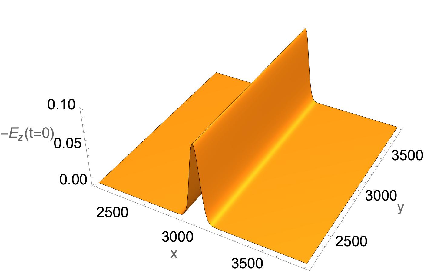
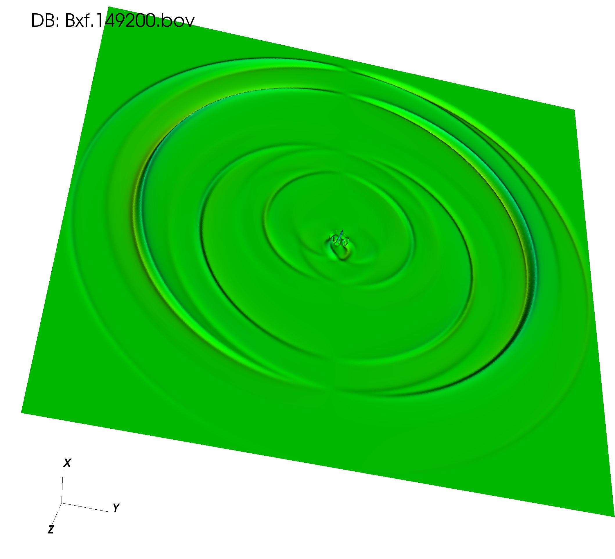
We now present detailed QLA simulations to the initial value problem of the scattering of a 1D electromagnetic pulse from a localized dielectric object. In particular we consider a 1D Gaussian pulse propagating in the -direction towards a localized dielectric object of refractive index . The initial pulse has non-zero field components ,, Fig. 1, and scatters from either a localized cylindrical dielectric, Fig. 2a, or a conic dielectric object, Fig 2b. These simulations were performed for .
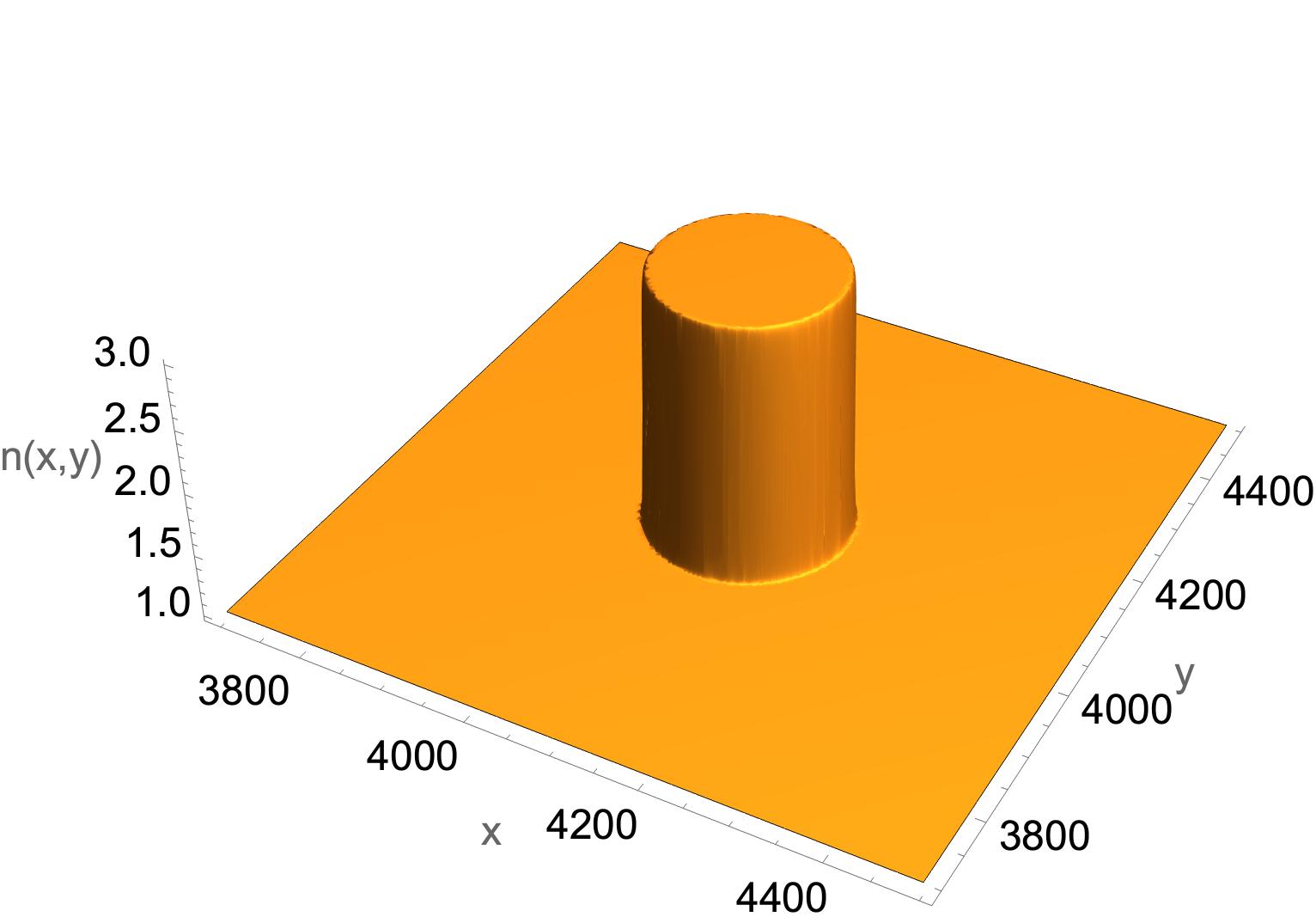
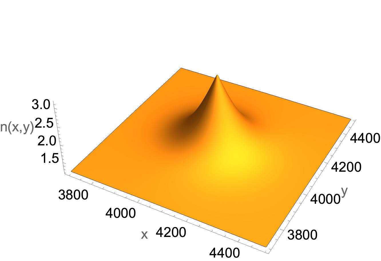
(a) localized dielectric cylinder (b) dielectric cone
It should be noted that QLA is an initial value algorithm : the refractive index profiles are smooth (e.g., hyperbolic tangents for the dielectric cylinder with boundary layer thickness lattice units) and so no internal boundary conditions are imposed at any time in the simulation.
4.1 Effects of broken symmetry
When the 1D pulse scatters off the dielectric object with refractive index the initial electric field spatial dependence now becomes a function , while the initial magnetic field will become a function . Now the scattered field has . Thus for , the scattered field must develop an appropriate . This is seen in our QLA simulations, even though the explicit discrete collide-stream algorithm only models asymptotically the Maxwell subset, Eq. (4). and this is exactly conserved in our QLA simulation.
Similarly for initial polarization. In this case the scattered magnetic field satisfies, for our 2D scattering in the x-y plane, exactly and no other magnetic field components are generated. Our discrete QLA recovers this exactly. However, in an attempt to preserve , the QLA will generate a non-zero field.
4.2 Scattering from localized 2D dielectric objects with refractive index
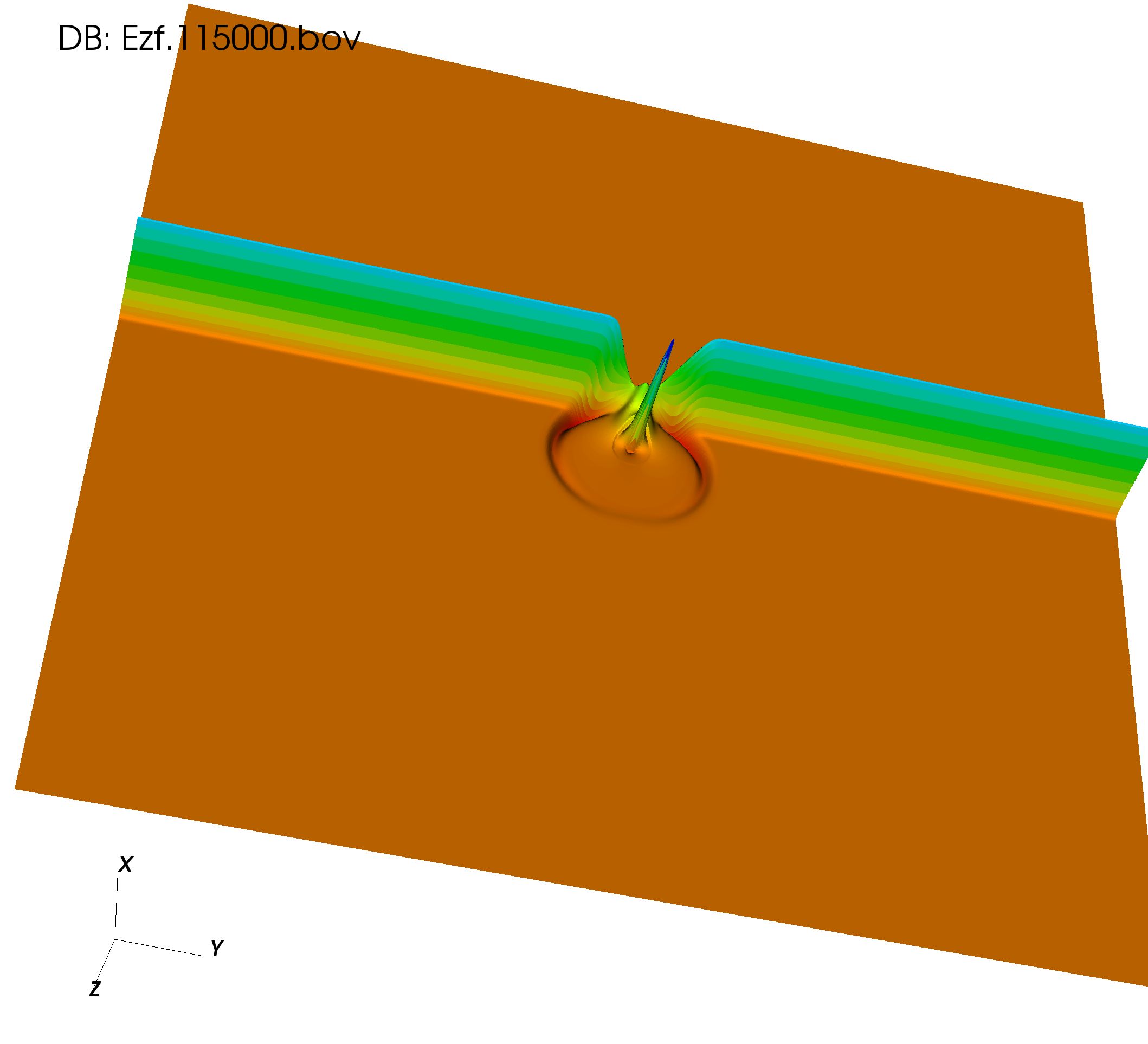
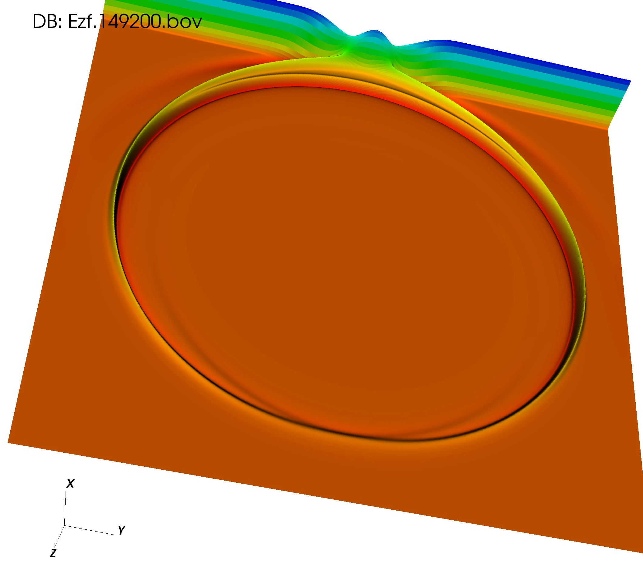
Consider a 1D pulse with polarization propagating in a vacuum towards a 2D dielectric scatterer. In Figs. 3-6 we consider the time evolution of the resultant scattered -field. The initial pulse is followed for a short time while it is propagating in the vacuum to verify that the QLA correctly determines its motion. As part of the pulse interacts with the dielectric object, the pulse speed within the dielectric itself is decreased by the inverse of the refractive index profiles, . The remainder of the 1D pulse propagates undisturbed since it is still propagating within the vacuum.
One sees in Fig. 3a a circular-like wavefront reflecting back into the vacuum, with its field out of phase as the reflection is occurring from a low to higher refractive index around the vacuum-cylinder interface. One does not find such a reflected wavefront when the pulse interacts with the conic dielectric, Fig. 3b.
(a) dielectric cylinder (b) dielectric cone
At , there is a major wavefront emanating from the back of the cylindrical dielectric, Fig. 4a. For the conic dielectric there is a major wavefront reflected from the apex of the conic dielectric, and this propagates out of the cone with little reflection, Fig. 4b.
(a) dielectric cylinder (b) dielectric cone
One clearly sees at that more wavefronts are being created because of the large refractive index gradients at the vacuum-cylinder dielectric boundary, while such gradients are missing from the vacuum-cone interface which leads to no new wavefronts in the scattering off the dielectric cone, Fig.5.
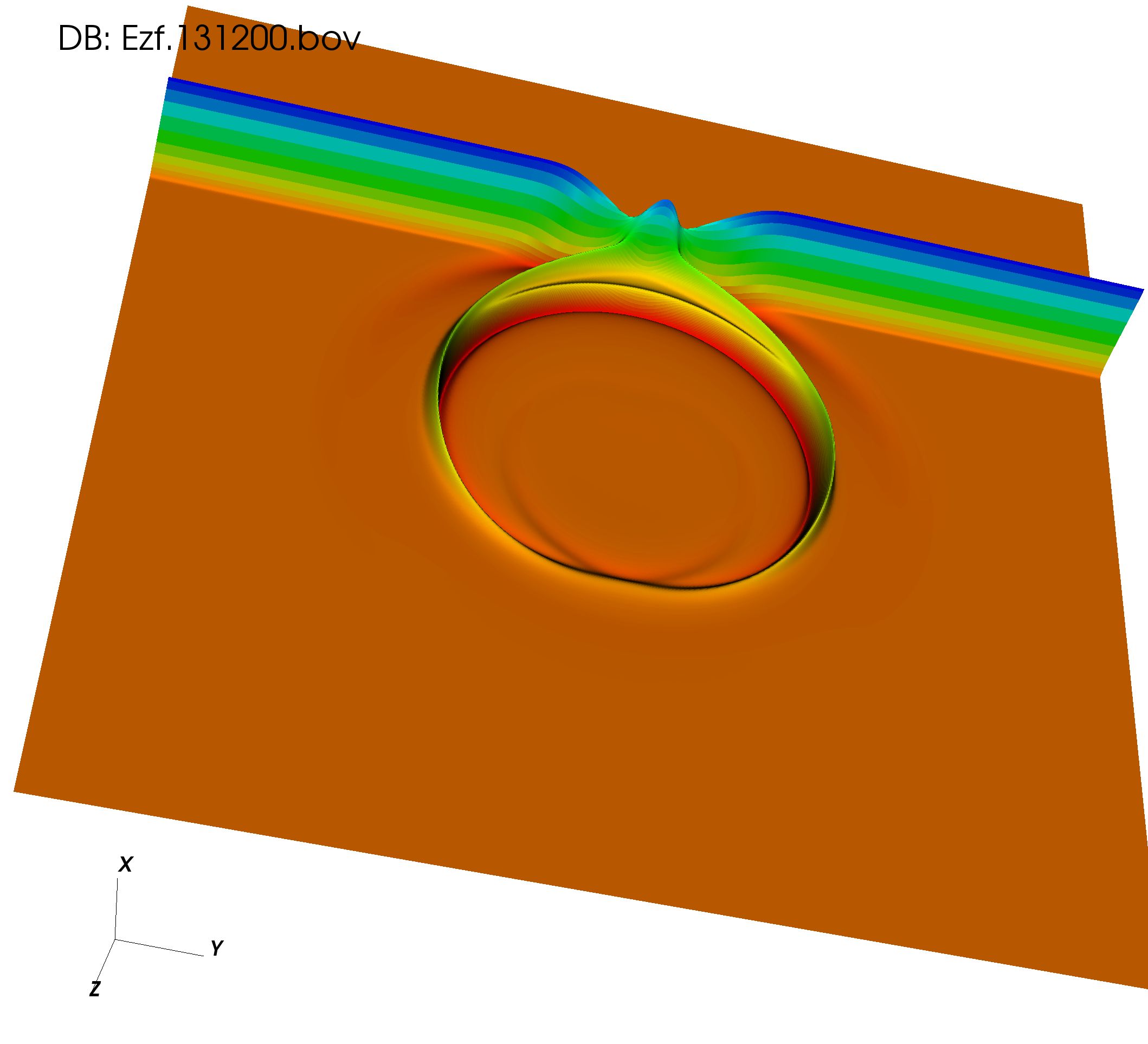
(a) dielectric cylinder (b) dielectric cone
At , the complex wavefronts are due to repeated reflections and transmissions from the cylinder dielectric, Fig. 5a. However, because of the slowly changing boundaries of the dielectric cone there are no more reflections and one sees only the outgoing wavefront from the pulses interaction with the region around the of the cone. Since the pulse reaches the apex of the cone before the corresponding pulse hits the backend of the dielectric cylinder, the conic wavefront is further advanced than that of the cylindrical wavefront, Fig. 5b.
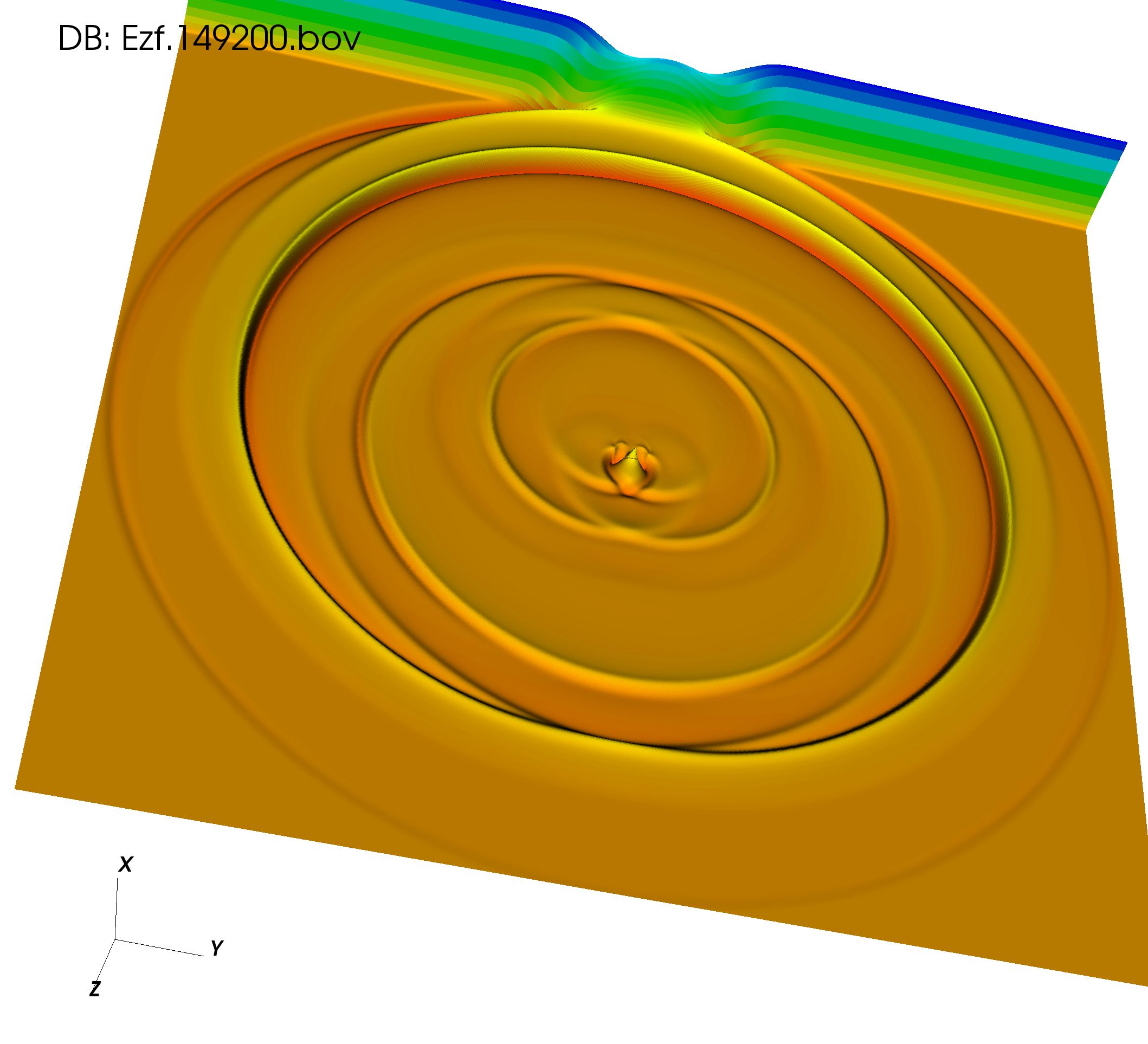
(a) dielectric cylinder (b) dielectric cone
4.2.1 Auxiliary fields and
For incident polarization and with 2D refractive index , the scattered electromagnetic fields will need to generate a field in order to have . In Fig. 6a and 6b we plot the self-generated field at and for scattering from the dielectric cylinder. It is also found that is typically zero everywhere in the spatial lattice except for a very localized region around the vacuum-dielectric boundary layer where the normalized reaches around 0.01 at very few isolated grid points.
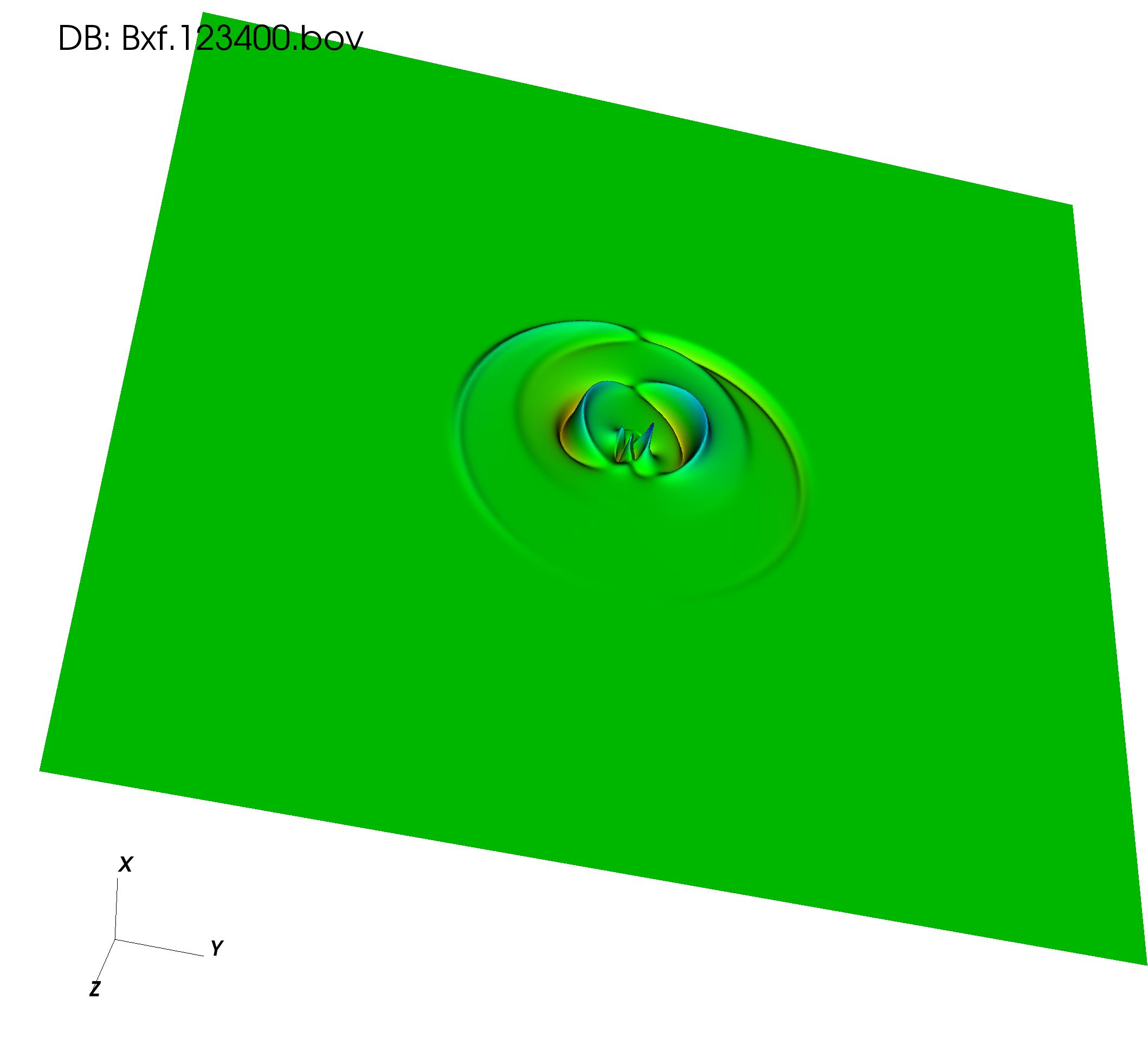
Scattering from dielectric cylinder: (a) t = 30k , (b) t = 37.8k
4.3 Time Dependence of on Perturbation Parameter
The discrete total electromagnetic energy . Eq. (30), is not constant since our current QLA is not totally unitary. However the variations in decrease significantly as . is a measure of the discrete lattice spacing. The maximal variations occur shortly after the 1D pulse scatters from the 2D dielectric object. For , this occurs around , with variations in the 5th decimal, Eq. (31). However, when one reduces by a factor of on the same lattice grid, then one recovers the same physics a factor of later in time since controls the speed of propagation in the vacuum. Thus the wallclock time of a QLA run is also increased by this factor of . We find, for , that the largest deviation in the total electromagnetic energy is now in the 8th decimal, Eq.. (31).
| (31) |
For , there is variation in in the 11th decimal.
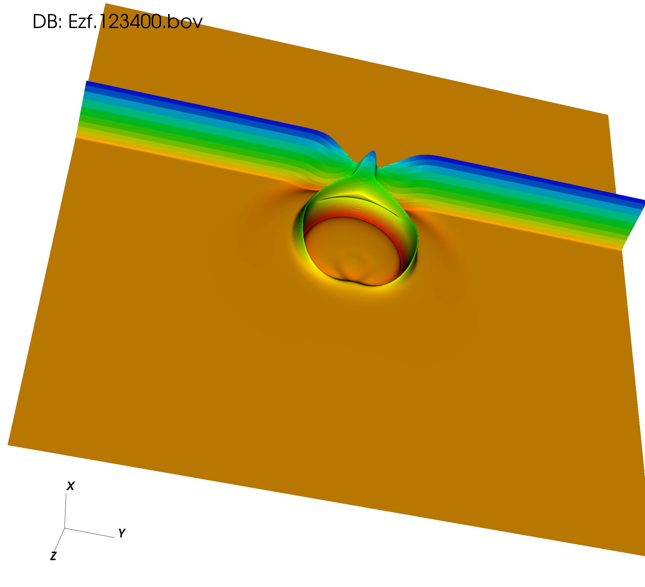
4.4 Multiple reflections/transmissions within dielectric cylinder
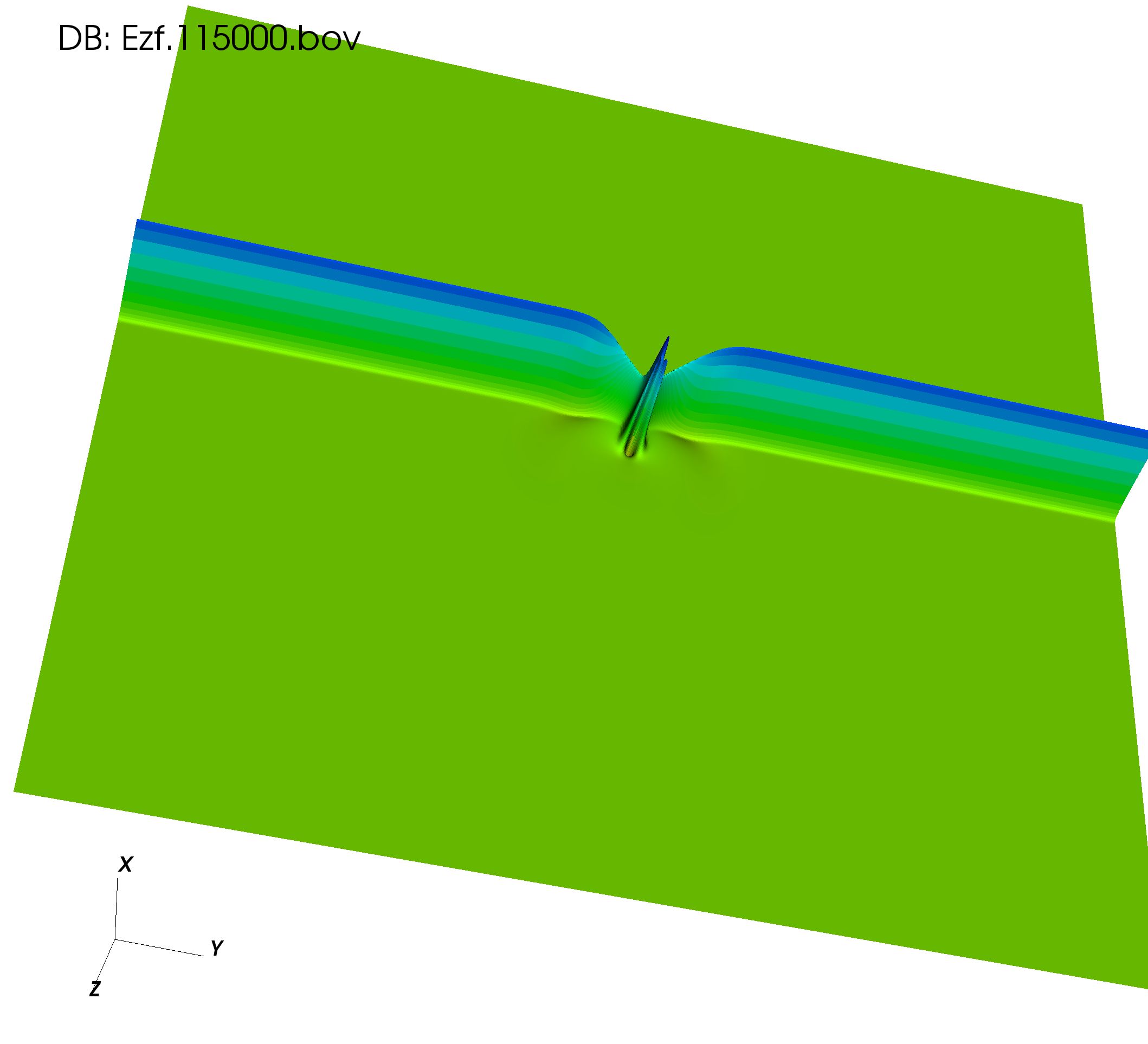
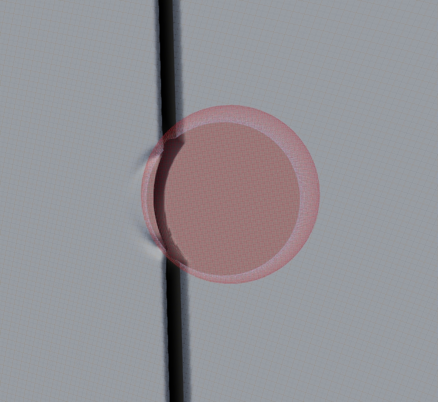
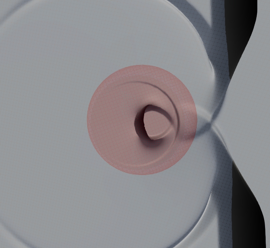
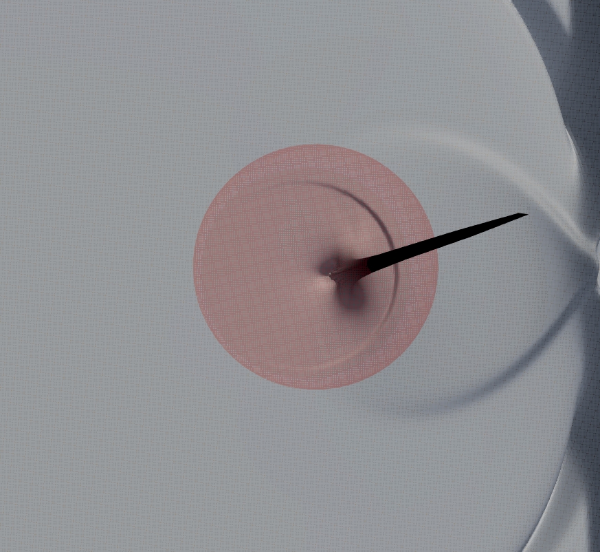
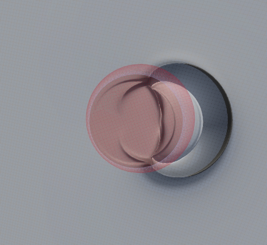
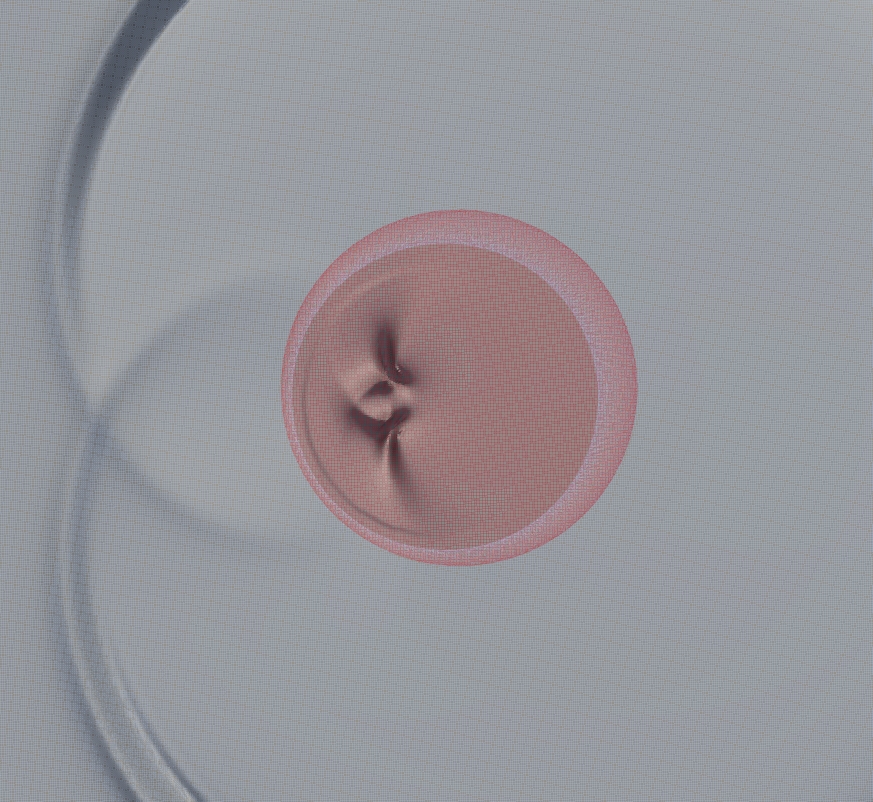
We now examine the scattered electromagnetic fields - particularly the polarization - within and in the vicinity of the dielectric cylinder. These plots complement the global scattered in Figs. 3a, 4a and 5a, but for better resolution we choose and a slightly different ratio of pulse width to dielectric cylinder diameter. In Figs 8 - 13, the perspective is looking down from above with the 1D pulse propagating from left to right (), seen as a dark vertical band. The dielectric cylinder appears as a pink cylinder with the smaller darker pink being the base of the cylinder. The time is expressed in normalized time : , where is the QLA time for .
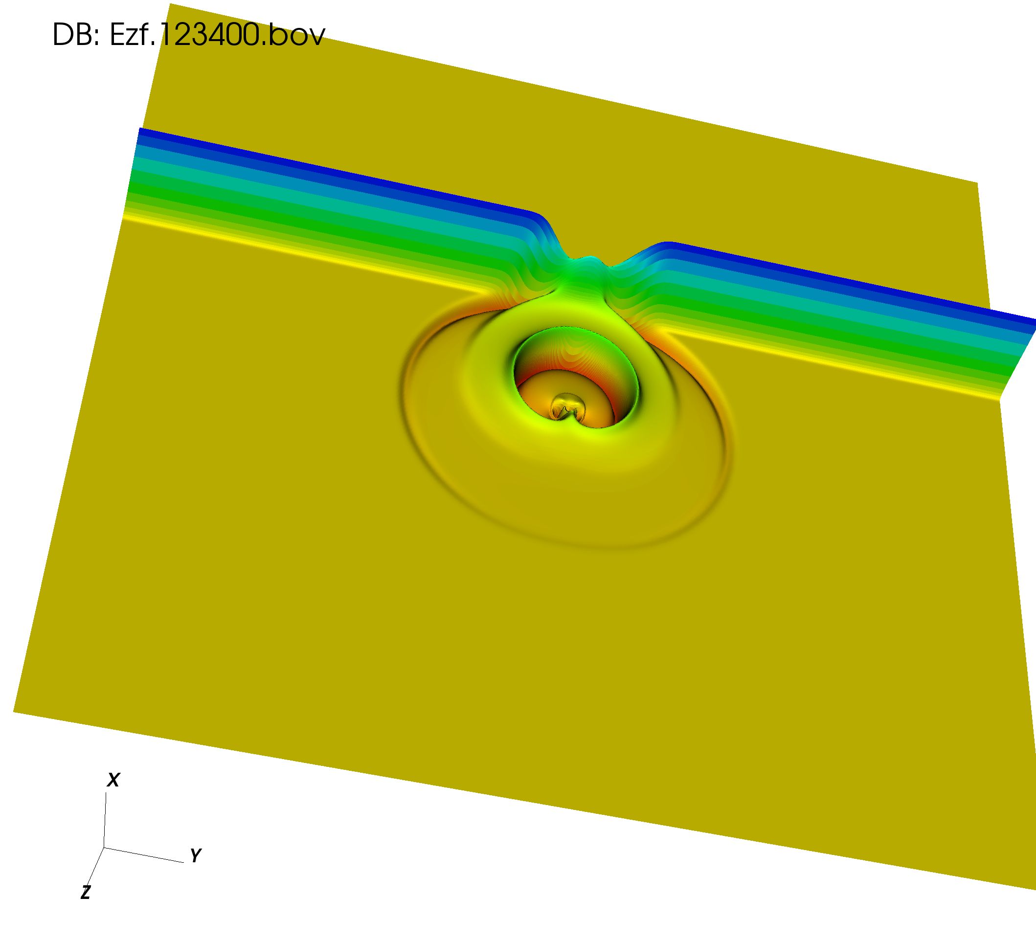
In Fig. 8a, at time , a part of the incident pulse has just entered the dielectric cylinder with the transmitted field starting to lag behind the main 1D vacuum pulse since . Also the reflected part of emanates from the two boundary points at the sharp vacuum-dielectric boundary and has undergone a -phase change because the incident 1D pulse is propagating from low to high refractive index. In Fig 8b the slower transmitted wavefront within the dielectric is very evident, as is the reflected part of back into the vacuum.
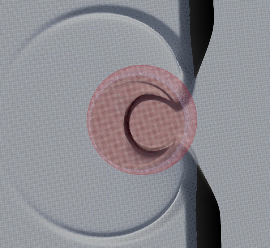
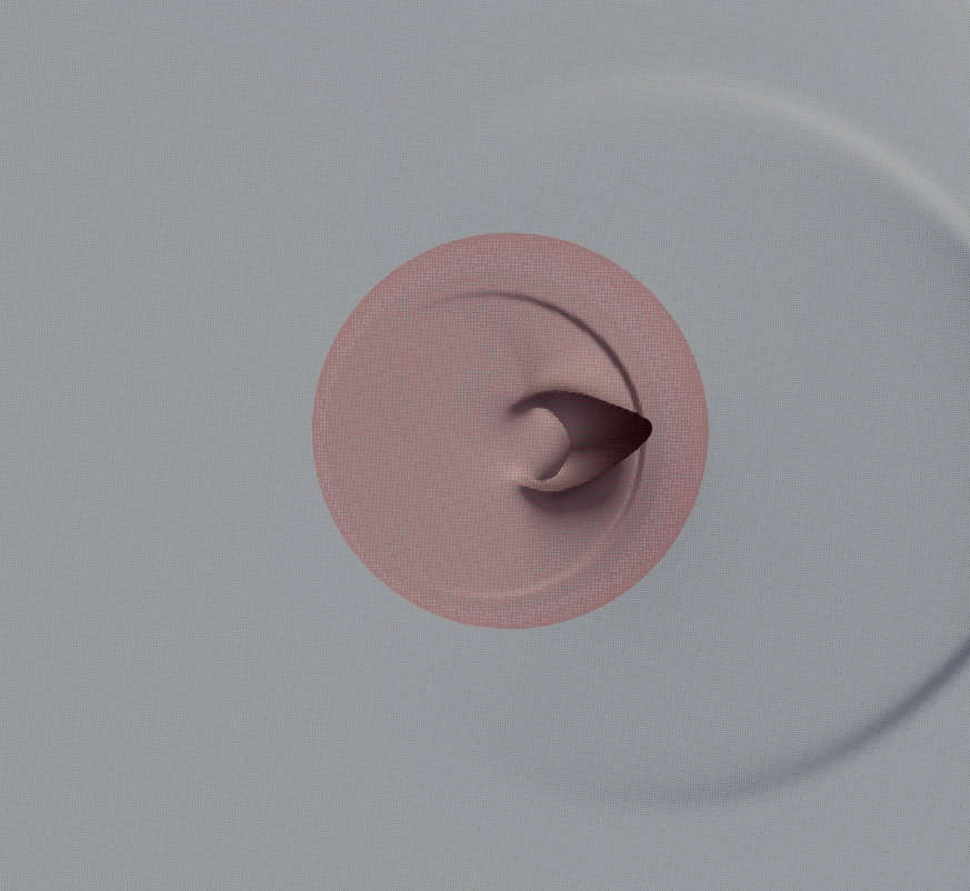
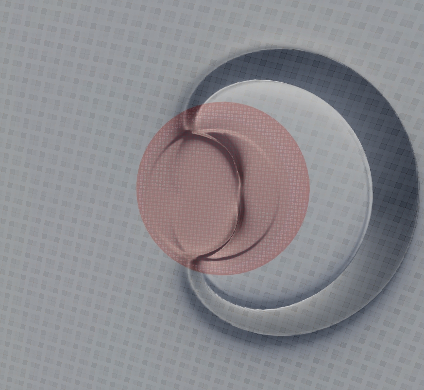
By , Fig 7b, the 1D pulse has propagated past the dielectric. The -field within the dielectric is now being focussed due to its motion towards the backend of the cylinder, with its increasing amplitude but reduced base. As it reaches the backend of the dielectric, part of will be transmitted into the vacuum while the other part will be reflected back into the dielectric - but now without any phase change since the pulse is propagating from high to low refractive index.
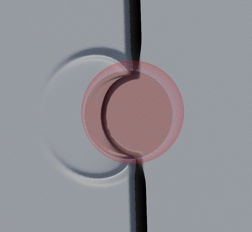
field: (a) t = 7.2k (b) t = 12k
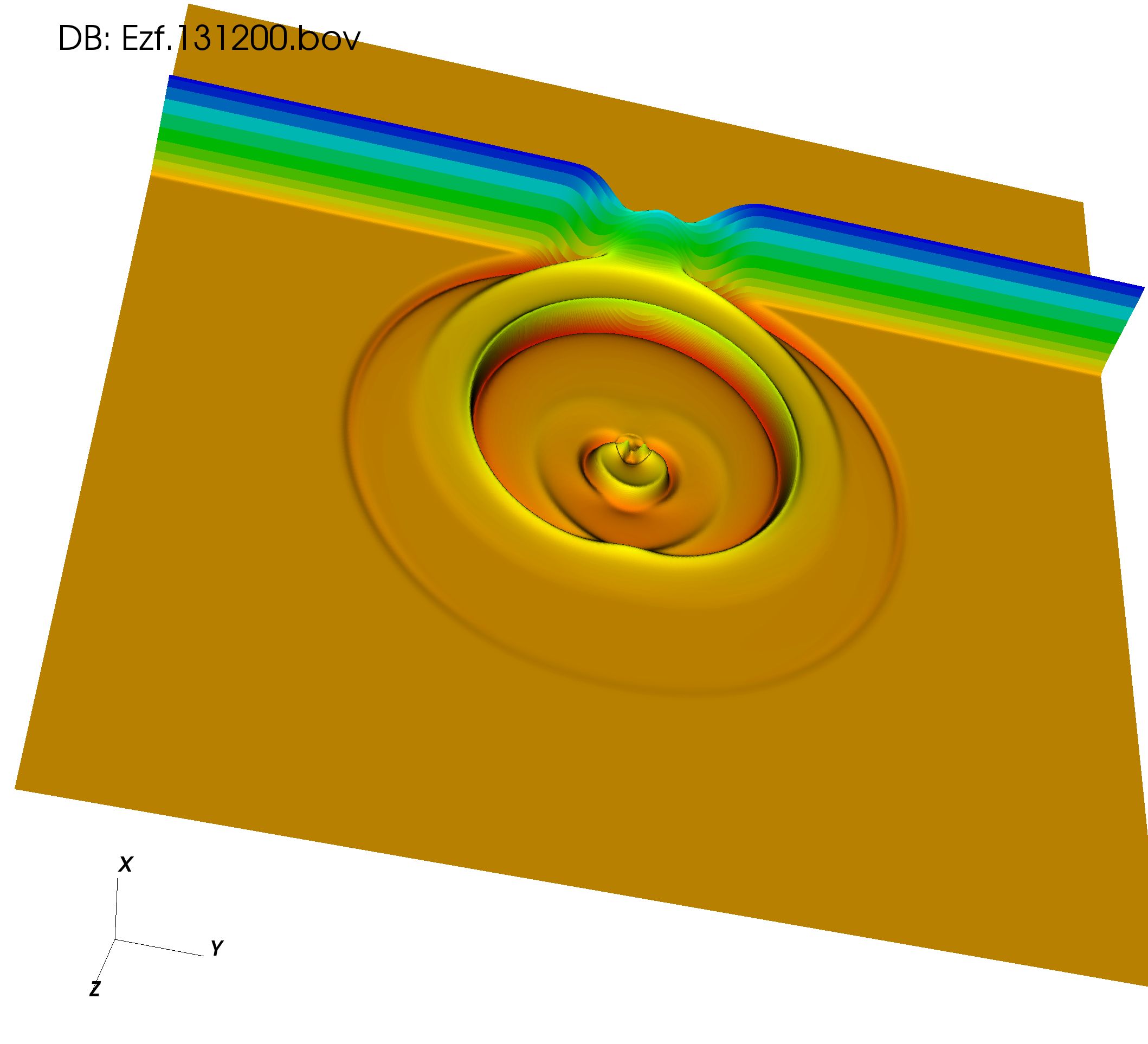
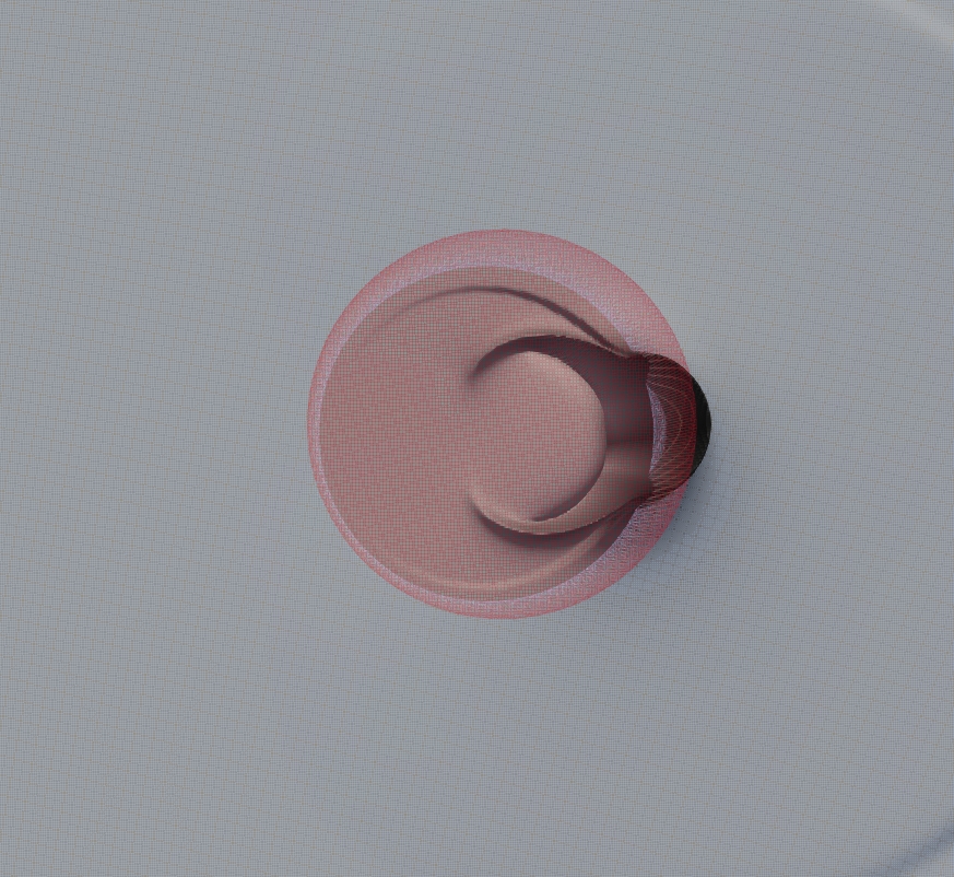
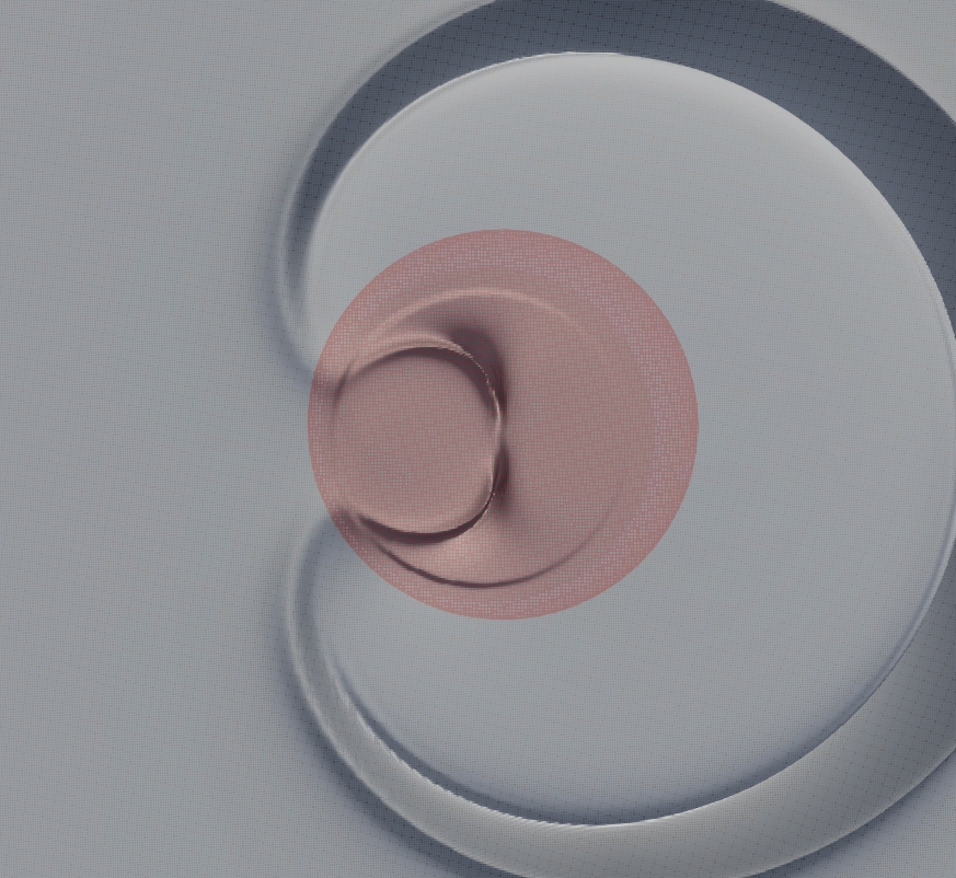
wavefronts at (a) t = 18k (b) t = 22.2k
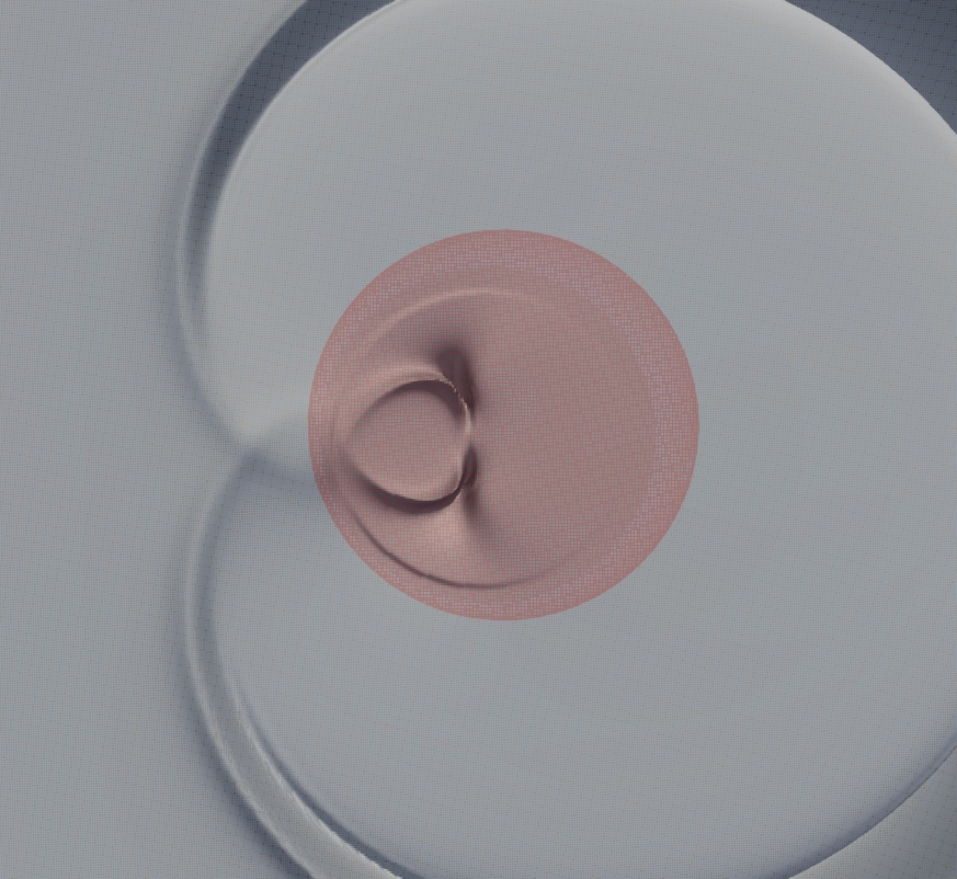
wavefronts at (a) t = 28.2k (b) t = 33k
wavefronts at (a) t = 38.4k (b) t = 43.2k
wavefronts at (a) t = 47.4k (b) t = 52.2k
wavefronts at (a) t = 55.8k (b) t = 60k
5 Dissipative Classical Systems, Open Quantum Systems and Kraus Representation
So far we have treated Maxwell equations as a closed system based on the energy conservation dictated from the Hermiticity and positive definiteness of the constitutive matrix , Eq. (7), since we have restricted ourselves to perfect materials. However, when we wish to consider actual materials there is dissipation. This immediately defeats any attempt to pursue a unitary representation in the original Hilbert space. The obvious question is : can we embed our dissipative system into a higher dimension closed Hilbert space, and thus recover unitary evolution in this new space and build an appropriate QLA that can be encoded onto quantum computers? To accomplish this, we resort to open quantum system theory [21] to describe classical dissipation as the observable result of interaction between our system of interest and its environment.
For a closed quantum system, the time evolution of a pure state is given by the unitary evolution from the Schrodinger equation : with unitary for the Hermitian Hamiltonian . The evolution of the density matrix, , is governed by the corresponding von Neumann equation : . The density matrix formulation is required when dealing with composite systems. Kraus realized that the density matrix retains its needed properties if one generalized its evolution operator to
| (32) |
where the only restriction on the set of so-called Kraus matrices is that the sum of is the identity matrix. The evolution of the density matrix, Eq. (32), is no longer unitary for .
The Kraus representation [21] is most useful when dealing with quantum noisy operations due to interaction with an environment. For those problems in which this noisy operation translates into a dissipative process, the Hamiltonian for the system in the Schrodinger representation has both a Hermitian part, , and an anti-Hermitian part, , that models the dissipation. A simple but non-trivial example is the Maxwell equations (without sources) for a homogeneous scalar medium with electrical losses,
| (33) |
with complex permittivity is the momentum operator. Introducing the Dyson map into Eq. (33) and after some algebraic manipulations the evolution equation can be written as
| (34) |
where the state vector , where is defined in Eq. (6). is the loss angle, is the phase velocity and are the Pauli matrices.
5.1 Classical Dissipation as a Quantum Amplitude Damping Channel
In symbolic form, the Maxwell equations with electric resistive losses, Eq. (34), can be written in the Schrodinger-form
| (35) |
where the Hamiltonians and are Hermitian, and the dissipative operator is anti-Hermitian and positive definite. The positive definiteness requirement for the specific case of propagation in a lossy medium translates to
| (36) |
In general the dissipative operator is relatively simple, and models the phenomenological or coarse-graining of the underlying microscopic dissipative processes.
We aim to represent the dissipation in the Schrodinger picture, Eq. (35), as an open quantum system S interacting with its environment . The full system, , is closed, and hence its time evolution is unitary. Let be this unitary operator, and the total density matrix with . We make the usual assumption that the initial total density matrix is separable into the system and into the environmental Hilbert spaces : . A quantum operation E on the open system of interest is defined as the map that propagates the open system density in time :
| (37) |
But under the conditions of initial separability, the action of the full unitary operators on the total density matrix will yield, after taking the trace over the environment,
| (38) |
Assuming a stationary environment, , Eq. (38) can be written
| (39) |
where . These operators will form a Kraus representation for the quantum operation E for an open system, Eq. (37), provided the so-called Kraus operators satisfy the extended ”unitarity” condition
| (40) |
Note that the individual Kraus operator need not be unitary. Based on this framework for open quantum systems we proceed to construct a physical unitary dilation for the combined system-environment by identifying dissipation as an amplitude damping operation, [21].
Let be the dimension of the system Hilbert space, and the dimension of the dissipative Hamiltonian , Eq. (35). We require , for optimal results but the dilation technique can be also applied to systems with . If the system was quantum mechanical in nature, then there can be a set of Kraus operators at most. The matrix representation of the total unitary dilation evolution operator consists of listing all the Kraus matrices in the first column block. The remaining columns must then be determined so that is unitary. This unitary dilation is equivalent to the Stinespring dilation theorem [25]. The advantage of the Kraus approach is that it avoids the need to actually know the physical properties of the environment.
Returning to the Schrodinger representation of the classical system Eq. (35), one can employ the Trotter-Suzuki expansion to
| (41) |
Even though is not unitary, is Hermitian and can be diagonalized by a unitary transformation
| (42) |
where are the dissipative rate eigenvalues of . Thus Eq. (41) becomes
| (43) |
where is
| (44) |
The non-unitary will be one of our Kraus operators, and it describes the physical dissipation in the open system. We must now introduce a second Kraus operator so that :
| (45) |
represents a transition that is not of direct interest. These Kraus operators are the multidimensional analogs of the quantum amplitude damping channel [21]: with corresponding to the dissipation processes, while corresponds to an unwanted quantum transition.
The block structure of the final unitary dilation evolution operator , corresponding to the non-unitary dissipation operator , consists of column blocks of the Kraus operators , and the remaining column blocks are of those matrices required to make unitary [21]:
| (46) |
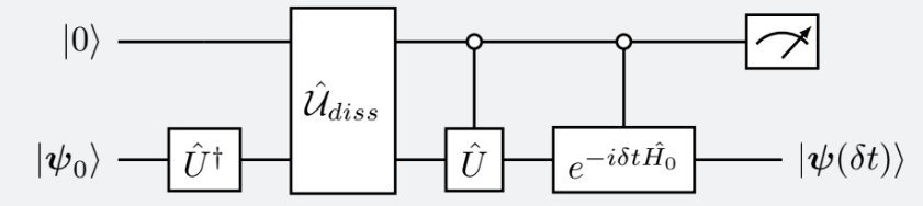
Thus, it can be shown that the evolution of the system and environment is given by
| (47) |
where measurement of the first qubit-environment by yields a state analogous to
. Finally, on taking the trace over the environment will yield the desired system state
The corresponding quantum circuit for Eq. (47) is shown in Fig. 14.
It is important to highlight that the implementation of the dissipative case is directly overlapping with the QLA framework. The QLA can be used to implement the part in Eq. (43) as proposed in the previous sections. Specifically for the lossy medium, the exponential operator of the term in Eq. (35) can be easily handled with QLA [12,13].
6 Conclusions
The Schrodinger-Dirac equations are the backbone of the work presented here on Maxwell equations both in lossless inhomogeneous and lossy dielectric media. In both cases, straightforward application of unitary algorithms fail : in the first case, somewhat surprisingly one finds that even though a Dyson map points to the required electromagnetic field variables in a tensor dielectric, its implementation has till now defied a fully unitary representation. Our current QLA approach requires some external non-unitary operators that recover the terms involving the spatial derivatives on the refractive indices of the medium. These sparse matrices can be modeled by the sum of a linear combination of unitaries (LCU), which can then be encoded onto a quantum computer [23, 24]. In the second case, handling dissipative systems immediately forces us to consider an open quantum system interacting with its environment. Typically this forces us into a density matrix formulation and a clever introduction of what is known as Kraus operators [21, 25]. The beauty of the Kraus representation is that even though the system of interest is interacting with the environment, the Kraus operators do not need detailed information on the environment.
We presented detailed 2D scattering of a 1D electromagnetic pulse off localized dielectric objects. QLA is an initial value scheme. No internal boundary conditions are imposed at the vacuum-dielectrix interface. For dielectrics will large spatial gradients in the refractive index, QLA simulations show strong internal reflection/transmission within the dielectric object. These lead to quite complex time evolution of wavefronts from the dielectric objects. On the other hand, for weak spatial gradients in the refractive index there are negligible reflections from the vacuum-dielectric interface. This is reminiscent of WKB-like effects in the ray tracing approximation.
In considering the dissipative counterpart, one must now include both the system and its environment in order to get a closed system with unitary representation. The Kraus operators are the most general scheme that will retain the properties of the density matrix in time. The probability of obtaining the desired non-unitary evolution of the open system after the measurement operator is
| (48) |
The form of the unitary operator , Eq. (42) implies that it can be decomposed into r two-level unitary rotations with Then, the quantum circuit implementation of requires CNOT - and quantum gates, so that there is a improvement in the circuit depth of . Our multidimensional amplitude damping channel approach is directly related to the Sz. Nagy dilation by a rotation. The Sz. Nagy dilation [26] is the minimal unitary dilation containing the original dissipative (non-unitary) system.
Acknowledgments
This research was partially supported by Department of Energy grants DE-SC0021647, DE-FG02-91ER-54109, DE-SC0021651, DE-SC0021857, and DE-SC0021653. This work has been carried out within the framework of the EUROfusion Consortium, funded by the European Union via the Euratom Research and Training Programme (Grant Agreement No. 101052200 - EUROfusion). Views and opinions expressed, however, are those of the authors only and do not necessarily reflect those of the European Union or the European Commission. Neither the European Union nor the European Commission can be held responsible for them. E. K. is supported by the Basic Research Program, NTUA, PEVE. K.H is supported by the National Program for Controlled Thermonuclear Fusion, Hellenic Republic. This research used resources of the National Energy Research Scientific Computing Center (NERSC), a U.S. Department of Energy Office of Science User Facility located at Lawrence Berkeley National Laboratory, operated under Contract No. DE-AC02-05CH11231 using NERSC award FES-ERCAP0020430.
7 References
[1] B. M. Boghosian & W. Taylor IV, ”Quantum lattice gas models for the many-body Schrodinger equation”, Internat. J. Modern Phys. C8, 705-716 (1997).
[2] [1] B. M. Boghosian & W. Taylor IV, ”Simulating quantum mechanics on a quantum computer”, Physica D 120, 30-42 (1998).
[3] J. Yepez & B.M. Boghosian, ”An efficient and accurate quantum lattice-gas model for the many-body Schroedinger wave equation,” Computer Physics Communications, 146, (2002) 280-294.
[4] G. Vahala, J. Yepez & L. Vahala, ”Quantum lattice gas representation of some classical solitons”, Phys. Lett A 310, 187-196 (2003)
[5] G. Vahala, L. Vahala & J. Yepez, ”Inelastic vector soliton collisions: a lattice-based quantum representation”, Pbhil. Trans: Math, Phys. and Eng. Sciences, Roy. Soc. 362, 1677-1690 (2004)
[6] J. Yepez, G. Vahala, L. Vahala & M. Soe, ”Superfluid turbulence from quantum Kelvin waves to classical Kolmogorov cascades”, Phys. Rev. Lett. 103, 084501 (2009)
[7] G. Vahala, J. Yepez, L. Vahala, M. Soe, B. Zhang & S. Ziegeler, ”Poincare recurrence and spectral cascades in three-dimensional quantum turbulence”, Phys. Rev. E 84, 046713 (2011)
[8] B. Zhang, G. Vahala, L. Vahala, &M. Soe, ”Unitary quantum lattice algorithm for two dimensional quantum turbulence”, Phys. Rev. E 84, 046701 (2011)
[9] G. Vahala, B. Zhang, J. Yepez, L. Vahala & M. Soe, ”Unitary qubit lattice gas representation of 2D and 3D quantum turbulence”, in Advanced Fluid Dynamics, ed. H. W. Oh, (InTech , 2012), Chpt 11., p. 239 - 272.
[10] L. Vahala, M. Soe, G. Vahala & J. Yepez, ”Unitary qubit lattice algorithms for spin-1 Bose Einstein condensates”, Rad. Effects Def. Solids 174, 46-55 (2019).
[11] G. Vahala, L. Vahala & M.Soe, ”Qubit unitary lattice algorithms for spin-2 Bose-Einstein Condensates,I - Theory and Pade Initial Conditions”, Rad. Effects Def. Solids 175, 102-112 (2020).
[12] G. Vahala, M. Soe & L. Vahala, ”Qubit unitary lattice algorithms for spin-2 Bose-Einstein Condensates,II - vortex reconnection simulations and non-Abelian vortices”, Rad. Effects Def. Solids 175, 113-119 (2020).
[13] S. Palpacelli & S. Succi ”The Quantum Lattice Boltzmann Equation: Recent Developments”, Comm. Computational Phys. 4, 980-1007 (2008).
[14] S. Succi, F. Fillion-Gourdeau, & S. Palpacelli, ”Quantum lattice Boltzmann is a quantum walk”, EPJ Quantum. Technol 2, 12 (2015).
[15] G. Vahala, L. Vahala, M. Soe, & A. K. Ram, ”Unitary quantum lattice simulations for Maxwell equations in vacuum and in dielectric media”, J. Plasma Phys. 86, 905860518 (2020).
[16] G. Vahala, J. Hawthorne, L. Vahala, A. K. Ram & M. Soe, ”Quantum lattice representation for the curl equations of Maxwell equations”, Rad. Effects and Defects in Solids 177, 85 (2022).
[17] G. Vahala, M. Soe, L.Vahala, A. Ram, E. Koukoutsis, & K. Hizanidis, ”Qubit Lattice Algorithm Simulations of Maxwell’s Equations for Scattering from Anisotropic Dielectric Objects”, e-print arXiv:2301.13601 (2023).
[18] A. Oganesov, G. Vahala, L. Vahala & M. Soe, ”Effect of Fourier transform on the streaming in quantum lattice gas algorithms”, Rad. Effects and Defects in Solids. 173, 169 (2018).
[19] S. A. Khan & R. Jagannathan, ”A new matrix representation of the Maxwell equations based on the Riemann-Silberstein-Weber vector for a linear inhomogeneous medium”, arXiv:2205.09907v2.
[20] E. Koukoutsis, K. Hizanidis, A. K. Ram & G. Vahala, ”Dyson maps and unitary evolution for Maxwell equations in tensor dielectric media”, Phys. Rev. A 107, 042215 (2023).
[21] M. A. Nielsen & I. L. Chuang, Quantum Computation and Quantum Information, Cambridge University Press, 2010 (10th Ed.)
[22] M. Suzuki, ”Generalized Trotter’s formula and systematic approximants of exponential operators and inner derivatives with applications to many-body probloems, Commun. Math. Phys. 51,183 (1976)
[23] A. M. Childs & N. Wiebe, ”Hamiltonian Simulation Using Linear Combinations of Unitary Operations”, Quantum Inf. and Comp. 12 , 901 (2012).
[24] A. M. Childs, R. Kothari & R. D. Somma, ”Quantum Algorithm for Systems of Linear Equations with Exponentially Improved Dependence on Precision”, SIAM J. on Comp. 46, 1920 (2017).
[25] W. F. Stinespring, ”Positive Functions on -Algebras”, Proc. Amer. Math. Soc. 6, 211 (1955).
[26] V. Paulsen, Completely Bounded Maps and Operator Algebras, Cambridge Univ. Press, 2003.