Quench dynamics of mass-imbalanced three-body fermionic systems in a spherical trap

The Ramsey signal is defined as the wavefunction overlap of the pre- and post-quench wavefunctions, it is given

where $\Psi_{\rm i}$ is the pre-quench wavefunction with energy $E_{\rm i}$ and $\Psi^{\prime}$ is the post-quench wavefunction. To obtain Eq. (21) we have inserted a complete set of post-quench eigenstates, $\Psi^{\prime}_{j}$, with energies $E_{j}$, where the sum over $j$ is a sum over all post-quench eigenstates Kerin and Martin (2020).

Since the COM wavefunction is unaffected by the quench the Ramsey signal is given

where indices with subscript i are the eigenvalues of the initial state and the unlabelled indices correspond to the post-quench eigenvalues. Note that $\bra{\phi_{ls}}\ket{\phi_{l^{\prime}\neq ls^{\prime}}}=0$, i.e. hyperangular states of different angular momenta are orthogonal.

To evaluate the Ramsey signal we need to evaluate the hyperradial integral $\bra{F_{qs}}\ket{F_{q^{\prime}s^{\prime}}}$ and the hyperangular integral $\bra{\phi_{ls}}\ket{\phi_{ls^{\prime}}}$.

The hyperradial integral is given Srivastava et al. (2003)

For $s=s^{\prime}$ and $q\neq q^{\prime}$ the hyperradial integral vanishes. Evaluating the hyperangular integral is not as straightforward as for the hyperradial integral due to the permutation operator. The hyperangle $\alpha$ is defined in terms of the Jacobi vectors $\vec{r}$ and $\vec{\rho}$, which are defined in terms of $\vec{r}_{1},\vec{r}_{2}$, and $\vec{r}_{3}$. We have defined $\vec{r}$ as being between particles one and two but it is possible to define $\vec{r}$ between any pair of particles. There are then three possible ways to define the Jacobi vectors for the three-body system, these Jacobi sets are related to one another by a “kinematic rotation” Nielsen et al. (2001), a coordinate transform in other words. We perform the hyperangular integral by taking advantage of these relations and “rotating” the terms acted upon by $\hat{P}_{23}$ into the same Jacobi set as the term not acted upon by $\hat{P}_{23}$ Fedorov and Jensen (1993, 2001); Braaten and Hammer (2006); Thøgersen (2009). However this restricts us to the $l=0$ case due to the presence of the spherical harmonic term making the coordinate transform intractable for $l>0$ as the hyperangular part of the wavefunction becomes a function of $\hat{\rho}$ in addition to $\alpha$. For the general mass case the overlap of $\phi_{0s}$ and $\phi_{0s^{\prime}}$ is given,

For $l=0$ Eq. (13) reduces to Werner (2008); Fedorov and Jensen (2001)

Note that combining Eqs. (25) and (26) for $\kappa=1$ (the equal mass case) does not give the same result as in Refs. Colussi (2019); Werner (2008) and only agrees when $s=s^{\prime}$ is one of the solutions to Eq. (16) for $\kappa=1$. This is because the latter references appropriately substitute Eq. (16) for $\kappa=1$ into the result for the hyperangular integral to simplify the expression.

However, for a general value of $\kappa$ we have to be more careful. For a specific $\kappa$ the $s$ eigenvalues produced by Eq. (16) are orthogonal to one another when Eq. (25) is evaluated only for that specific value of $\kappa$, i.e. the $s$-eigenspectrum for $\kappa=x$ produces an orthogonal set of states only when Eq. (25) is evaluated using $\kappa=x$. However, the non-interacting values of $s$ ($s=4,6,8,\dots$) are orthogonal to one another whatever the value of $\kappa$.

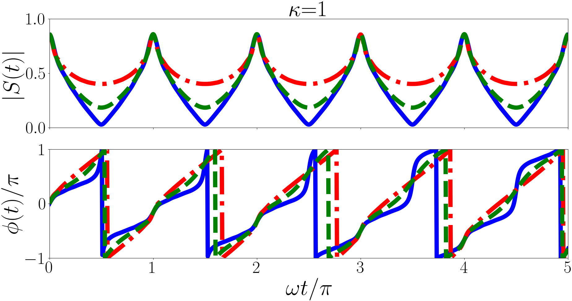
Now that we can calculate the wavefunction overlaps we can evaluate the Ramsey signal for the forwards and backwards quenches for any initial state with $l=0$ and any mass imbalance. In Figs. 1 and 2 we plot the forwards and backwards quenches respectively for a variety of $\kappa$ and initial states.

Before we discuss the properties of the Ramsey signals, in Figs. 1 and 2, it is worth exploring what we may expect in a general sense. Assuming in Eq. (22) that the sum is dominated by a few terms, the general form for $S(t)$ can be represented by $S(t)\approx Ae^{-ait}+Be^{-bit}+Ce^{-cit}$. The magnitude of the signal oscillates with angular frequencies $(a-b),(b-c),(a-c)$ with the more heavily weighted terms being more significant. However the phase of the signal is dominated by the angular frequencies of the most heavily weighted terms not the difference between angular frequencies of different terms. In our case the angular frequencies ($a,b,c,\dots$) are the differences between a post-quench eigenenergy and the initial energy, and the difference between the angular frequencies ($(a-b),(b-c),(a-c),\dots$) is the difference between different post-quench eigenenergies.

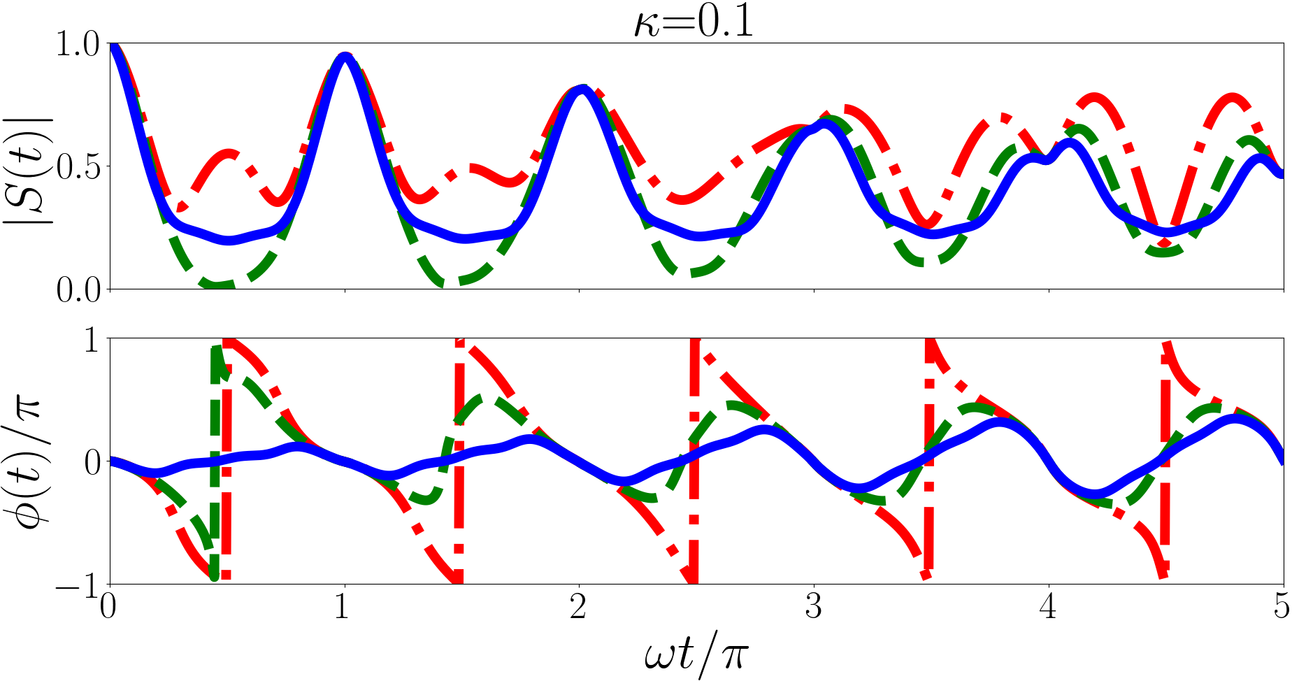
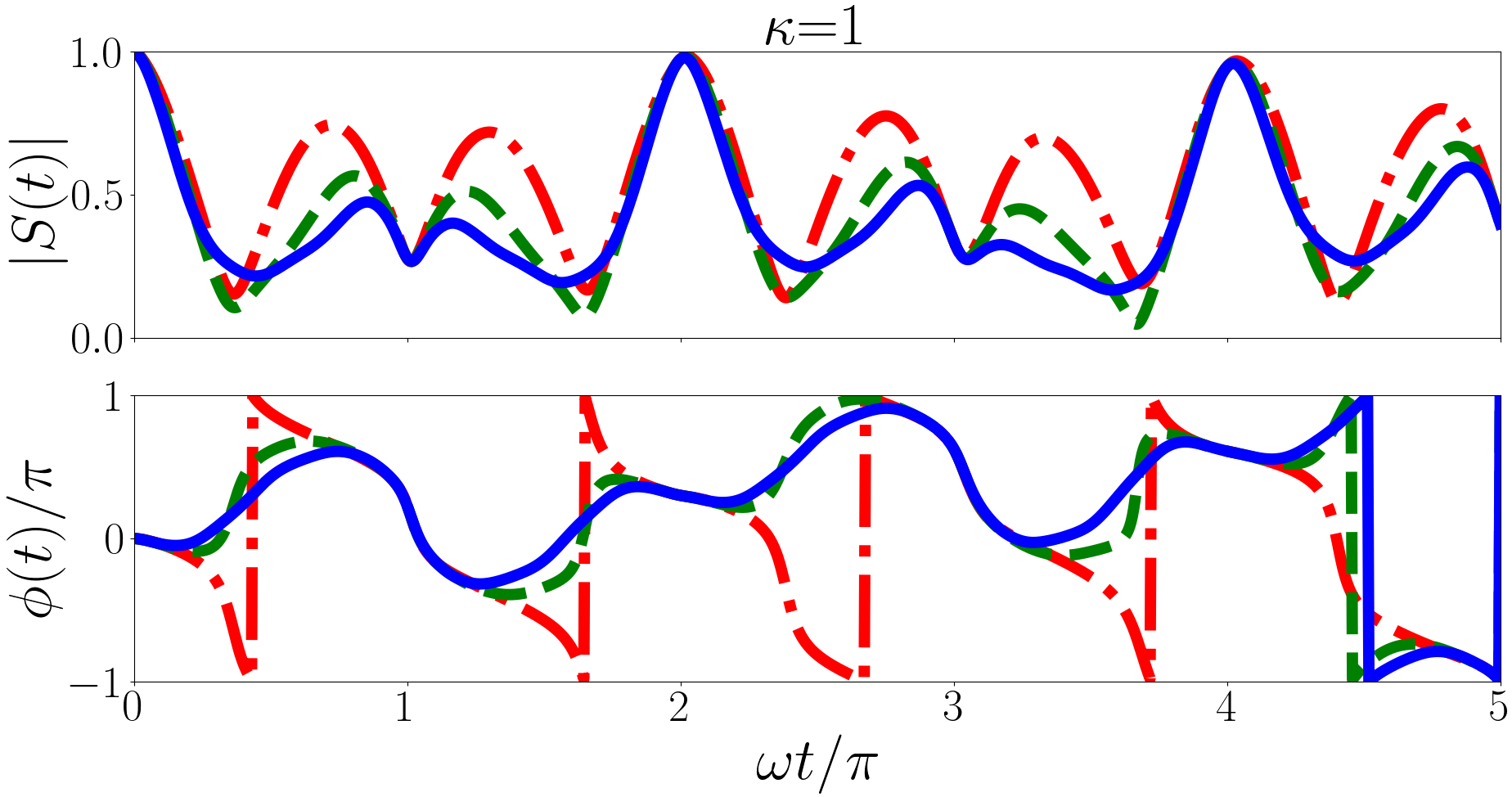
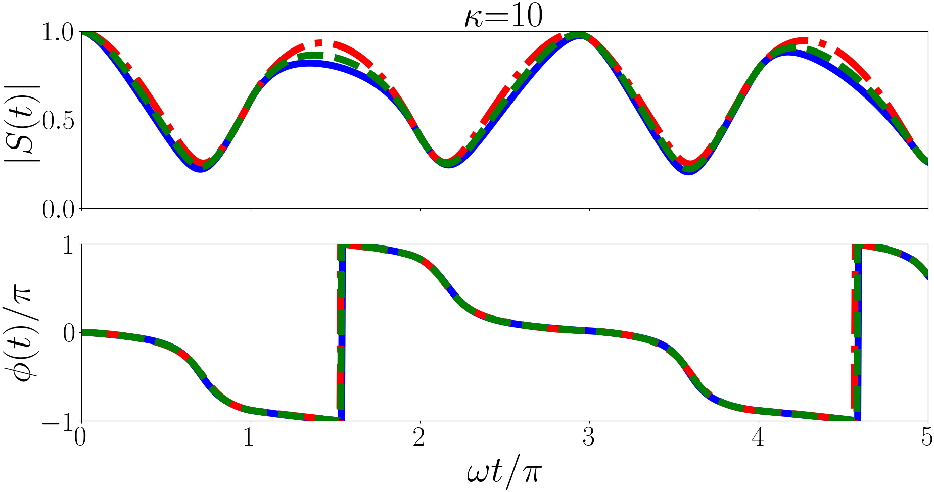
In Fig. 1 we plot the Ramsey signals of the forwards quench for a variety of initial states and mass imbalances. We find an irregularly repeating Ramsey signal, this is in contrast to similar calculations performed for the two-body problem Kerin and Martin (2020) where the signal is periodic with period $\pi/\omega$. This irregular periodicity arises from the unitary $s$-eigenspectrum. In this case angular frequencies of each term in Eq. (22) are irrational and so are the differences between them, in general. These irrational angular frequencies lead to the irregular phase and magnitude.

For the $\kappa=0.1$ (heavy impurity) forwards quench the most heavily weighted terms in Eq. (22) for the $(q_{\rm i},s_{\rm i})=(0,4)$ initial state (red line in the upper panel of Fig. 1 are the $|\bra{F_{0,4}\phi_{0,4}}\ket{F_{0,2.004}\phi_{0,2.004}}|^{2}\approx 0.539$, $|\bra{F_{0,4}\phi_{0,4}}\ket{F_{0,5.817}\phi_{0,5.817}}|^{2}\approx 0.134$ and $|\bra{F_{0,4}\phi_{0,4}}\ket{F_{1,2.004}\phi_{0,2.004}}|^{2}\approx 0.179$ terms. The corresponding angular frequencies are $\approx-2\omega$, $\approx 1.8\omega$, $\approx 0.004\omega$ respectively. Hence the phase displays features with a period of $\approx\pi/\omega$, and the magnitude has three main modes with periods $\approx 0.5\pi/\omega$, $\pi/\omega$ and $\approx 1.1\pi/\omega$.

For the $\kappa=1$ (equal mass) forwards quench the most significant terms for the $(q_{\rm i},s_{\rm i})=(0,4)$ initial state are $|\bra{F_{0,4}\phi_{0,4}}\ket{F_{0,2.166}\phi_{0,2.166}}|^{2}\approx 0.499$, $|\bra{F_{0,4}\phi_{0,4}}\ket{F_{0,5.127}\phi_{0,5.127}}|^{2}\approx 0.297$, and $|\bra{F_{0,4}\phi_{0,4}}\ket{F_{1,2.166}\phi_{1,2.166}}|^{2}\approx 0.13$. The corresponding angular frequencies are $\approx-1.8\omega$, $\approx 1.1\omega$ and $\approx 0.17\omega$ respectively. The phase is then dominated by a mode with period $\approx 1.1\pi/\omega$ and the magnitude is dominated by modes with periods $\approx 2\pi/3\omega,\pi/\omega$ and $\approx 2\pi/\omega$.

For the $\kappa=10$ (light impurity) forwards quench the most significant terms for the $(q_{\rm i},s_{\rm i})=(0,4)$ initial state are $|\bra{F_{0,4}\phi_{0,4}}\ket{F_{0,3.3169}\phi_{0,3.3169}}|^{2}\approx 0.607$, and $|\bra{F_{0,4}\phi_{0,4}}\ket{F_{0,4.707}\phi_{0,4.707}}|^{2}\approx 0.350$. The corresponding angular frequencies are $\approx-0.7\omega/\pi$ and $\approx 0.7\omega/\pi$ respectively hence the phase has an approximate periodicity of $2.8\pi/\omega$ and the magnitude has a period of $\approx 1.4\pi/\omega$.

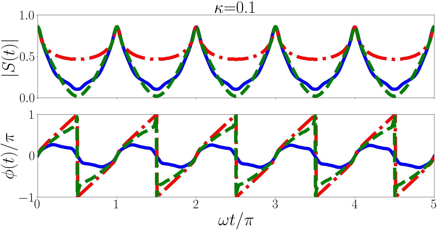
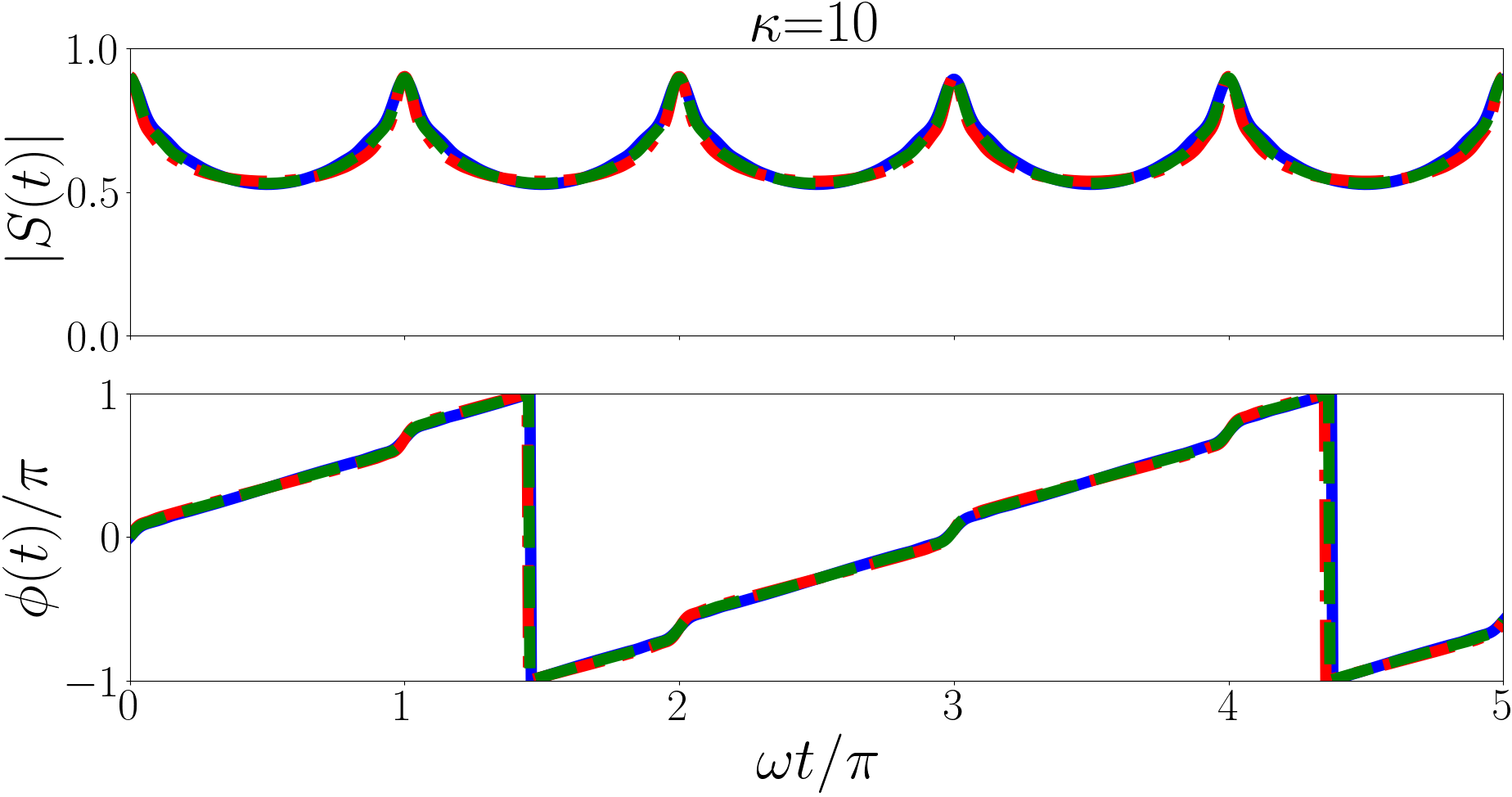
In Fig. 2 we plot the Ramsey signals of the backwards quench for a variety of initial states and mass imbalances. We find a strongly periodic magnitude. In the non-interacting regime we have $s=4,6,8,\dots$ for every value of $\kappa$. This means that every oscillatory term in the magnitude has an angular frequency that is a multiple of two, hence the period of $\pi/\omega$. However the behaviour of the phase is still dominated by the largest terms in the summation. For $\kappa=0.1$ (heavy impurity) and $(q_{\rm i}=0,s_{\rm i}=2.00449\dots)$ the largest term is $|\bra{F_{0,2.004}\phi_{0,2.004}}\ket{F_{0,4}\phi_{0,4}}|^{2}\approx 0.539$ and this defines the period of $\approx\pi/\omega$ we see in the phase. Similarly for $\kappa=1$ (equal mass) and $(q_{\rm i}=0,s_{\rm i}=2.166\dots)$ the largest term is $|\bra{F_{0,2.166}\phi_{0,2.166}}\ket{F_{0,4}\phi_{0,4}}|^{2}\approx 0.499$ defining a period of $\approx 1.1\pi/\omega$ for the phase, and for $\kappa=10$ (light impurity) and $(q_{\rm i}=0,s_{\rm i}=3.3169\dots)$ the largest term is $|\bra{F_{0,3.3169}\phi_{0,3.3169}}\ket{F_{0,4}\phi_{0,4}}|^{2}\approx 0.607$ defining a period of $\approx 2.8\pi/\omega$ for the phase.

The Ramsey signal is not the only quench observable we investigate. We can also calculate the expectation value of $\tilde{R}$, i.e. the particle separation.

The expectation value of $\tilde{R}(t)$ is given

where $\Psi_{\rm i}$ is the initial pre-quench state with energy $E_{\rm i}$ and $\Psi$ is the post-quench state. $\Psi^{\prime}_{j}$ and $\Psi^{\prime}_{j^{\prime}}$ are eigenstates of the post-quench system with eigenenergy $E_{j}$ and $E_{j^{\prime}}$ respectively, with the sum over $j$ and $j^{\prime}$ taken over all post-quench eigenstates.

The COM wavefunction is independent of the interparticle interaction and does not change when the system is quenched and does not impact the post-quench dynamics. Due to the hyperangular wavefunction’s orthogonality in $s$, two sums over $s$ and $s^{\prime}$ collapse into a single sum over $s$. Hence $\langle\tilde{R}(t)\rangle$ is given

All integrals required for calculating Eq. (28) are calculated in Sec. III.1 except for $\bra{F_{q^{\prime}s}}\tilde{R}\ket{F_{q^{\prime}s}}$. This is given Srivastava et al. (2003)

This result combined with the results of Sec. III.1 allows us to calculate $\langle\tilde{R}(t)\rangle$ for the forwards and backwards quench for any initial state with $l=0$ and any mass imbalance.

In Sec. III.1 we note that the magnitude and phase of the Ramsey signal for the forwards quench is irregular and this is because the $s$ eigenvalues are irrational at unitarity. Additionally the phase for the backwards quench is also irregular and this is due to the irrationality of $s_{\rm i}$. However the angular frequencies of the terms in Eq. (28) are always even integers because the $s$ contributions to the energies cancel leaving angular frequencies proportional to $(2q^{\prime}-2q)\omega$ and $q,q^{\prime}\in\mathbb{Z}_{\geq 0}$. This results in the angular frequency of every term in the summation being a multiple of $2\omega$ causing $\langle\tilde{R}(t)\rangle$ to have a period of $\pi/\omega$ in both the forwards and backwards quench.

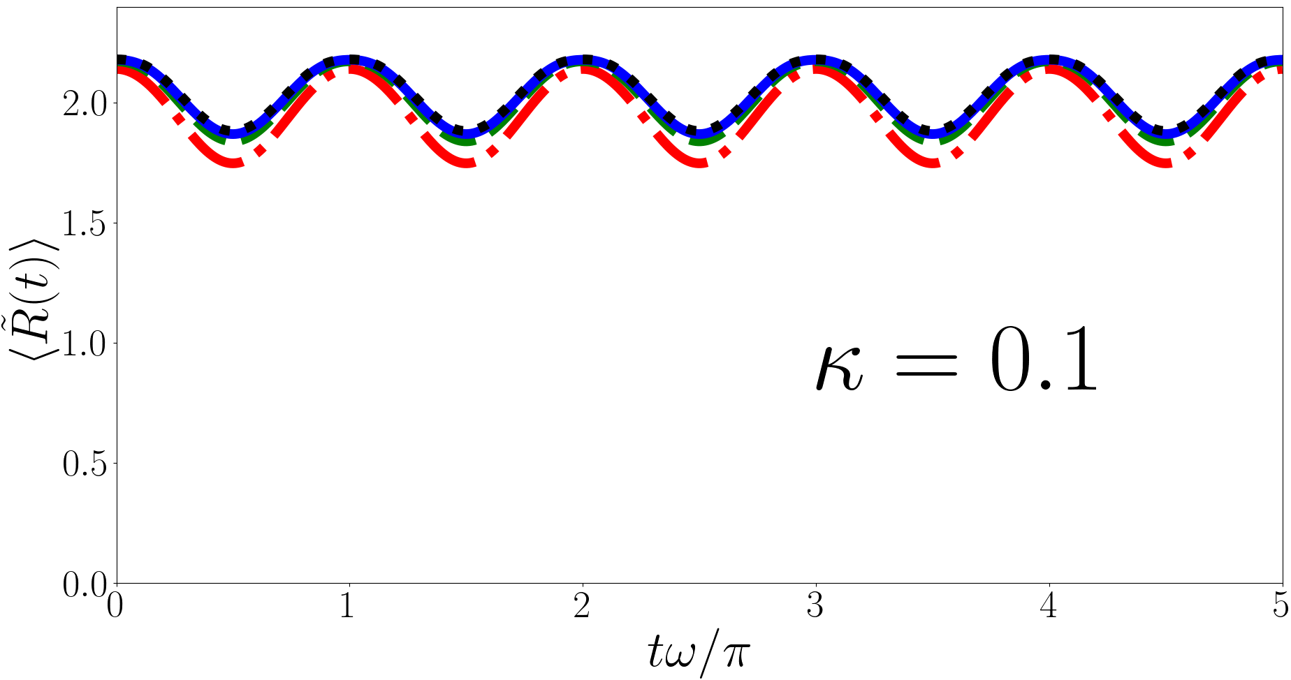
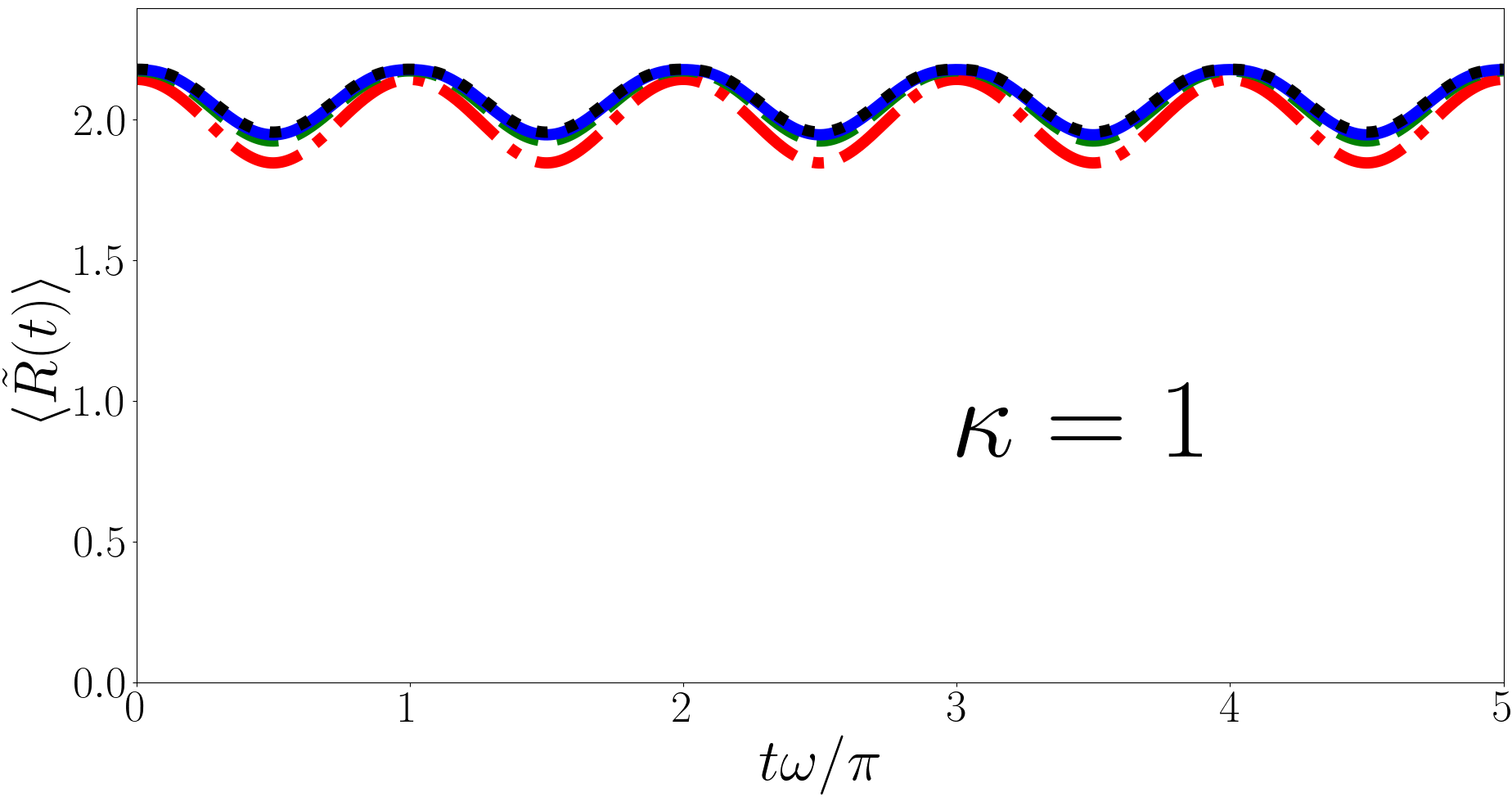
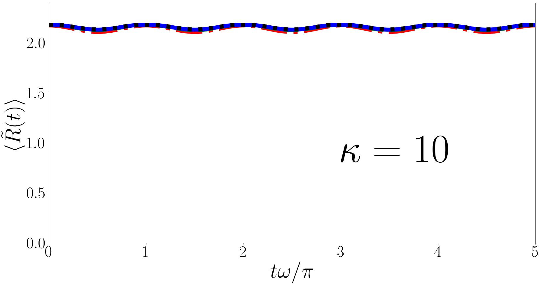
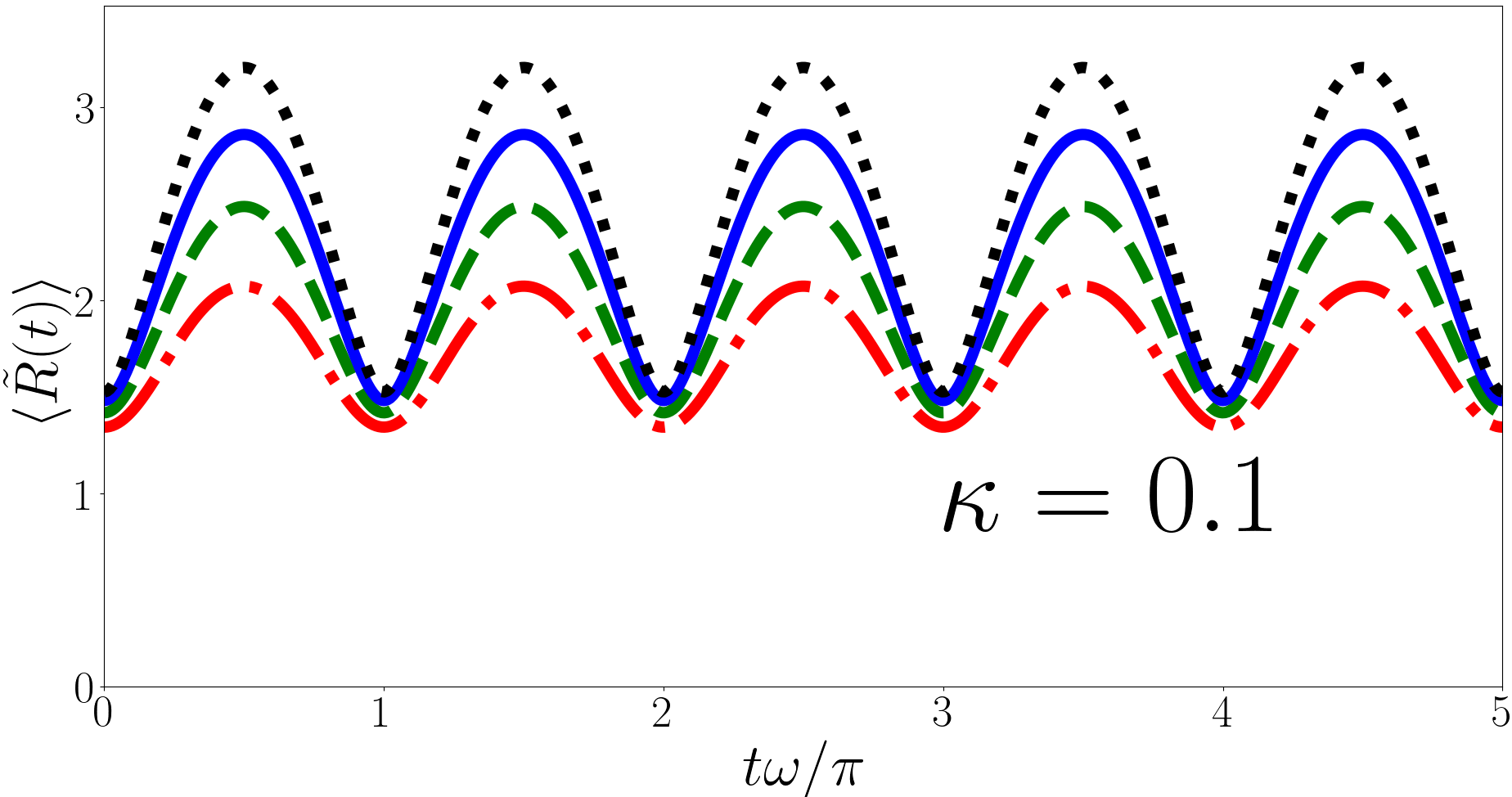
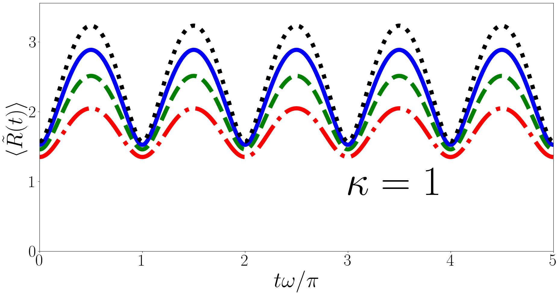
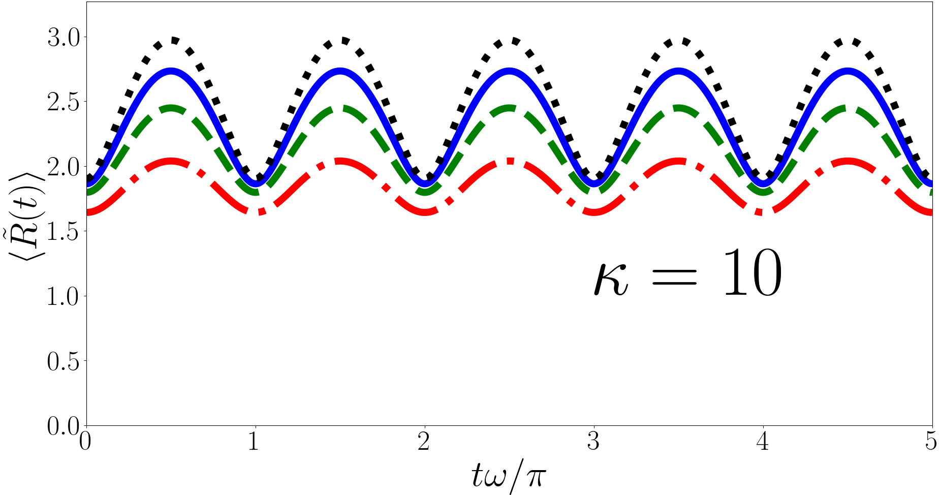
In Fig. 3 we have plotted $\langle\tilde{R}(t)\rangle$ for the forwards quench for $\kappa=0.1$, $\kappa=1$ and $\kappa=10$ (heavy impurity, equal mass, and light impurity) in the upper, middle and lower panels respectively. For each $\kappa$ we have taken the initial state to be the ground state and calculated the sum in Eq. (28) over $q$, $q^{\prime}$ and $s$ up to $N_{\rm max}=3,6,12$ and $24$, where $N_{\rm max}$ is the number of terms in each individual sum, so there are $N_{\rm max}^{3}$ terms total. In each case we find that the results for $\langle\tilde{R}(t)\rangle$ have converged at $N_{\rm max}=24$. As discussed above $\langle\tilde{R}(t)\rangle$ oscillates with a period $\pi/\omega$.

Additionally we observe that as $\kappa$ increases (impurity becomes lighter) the amplitude of the oscillation decreases. In the $\kappa\rightarrow\infty$ limit the unitary $s$-eigenspectrum approaches $s\rightarrow 4,6,8\dots$ Kerin and Martin (2022) and the initial non-interacting ground state overlaps perfectly with the unitary ground state. As such the amplitude decreases as $\kappa$ increases until eventually $\langle\tilde{R}\rangle$ reaches a constant value of $2.18\dots$ which is $\langle\tilde{R}\rangle$ for $q=0$, $s=4$. This is also $\langle\tilde{R}(t=0)\rangle$, the maximum particle separation does not change with $\kappa$ but the minimum increases to decrease the amplitude. Conversely in the $\kappa\rightarrow 0$ (heavy impurity) limit the unitary $s$-eigenspectrum approaches $s\rightarrow 2,6,10,14\dots$, analytically this presents a problem. The non-interacting ground state, $s_{\rm i}=4$, is orthogonal to the unitary $s$-eigenspectrum because it is a subset of the non-interacting eigenspectrum, except $s=2$ which is forbidden for $l=0$ because it causes the hyperangular part of the wavefunction to be zero. Numeric investigations for $\kappa$ as small as $10^{-3}$ imply that the minimum $\langle\tilde{R}(t)\rangle$ asymptotes to $\approx 1.7\dots$ as $\kappa$ becomes very small. The maximum particle separation remains at $2.18\dots a_{\mu}$ whatever the value of $\kappa$ because the initial non-interacting state does not depend on $\kappa$.

In Fig. 4 we have considered $\langle\tilde{R}(t)\rangle$ for the backwards quench for the $\kappa=0.1$, $\kappa=1$ and $\kappa=10$ cases, (heavy impurity, equal mass, and light impurity) in the upper, middle and lower panels respectively. For each $\kappa$ we have taken the initial state to be the ground state and calculated the sum in Eq. (28) over $q$, $q^{\prime}$ and $s$ up to $N_{\rm max}=3,6,12$ and $24$. Similar to $r=|\vec{r}_{1}-\vec{r}_{2}|$ in the two body case Kerin and Martin (2020) we observe in the backwards quench that the particle separation diverges away from $\omega t=n\pi$. For the three-body case we find that $\langle\tilde{R}[t=(n+1/2)\pi/\omega]\rangle$ diverges logarithmically with $N_{\rm max}$. More specifically we find that if the number of terms in the sums over $q$ and $q^{\prime}$ is fixed then as more terms are included in the sum over $s$ $\langle\tilde{R}(t)\rangle$ converges. The divergence in $\langle\tilde{R}(t)\rangle$ comes from the sums over $q$ and $q^{\prime}$ and therefore from the hyperradial wavefunction. This divergence warrants further scrutiny, to this end we investigate the evolution of the probability distribution of $R(t)$,

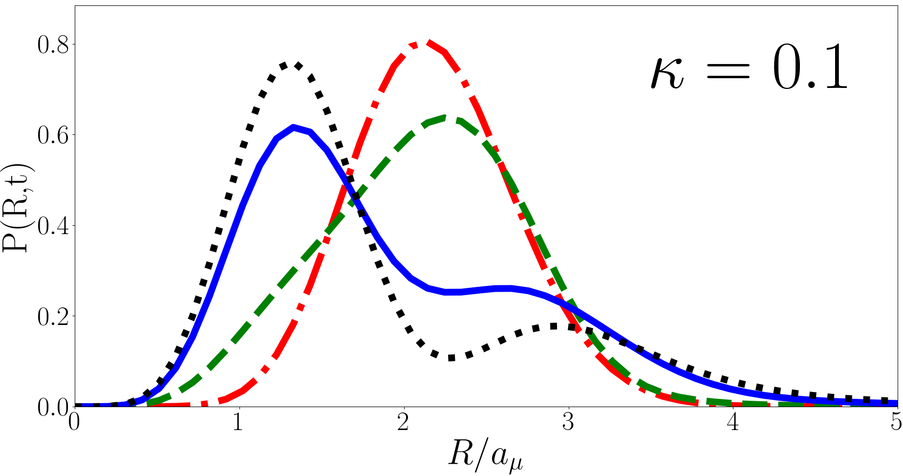
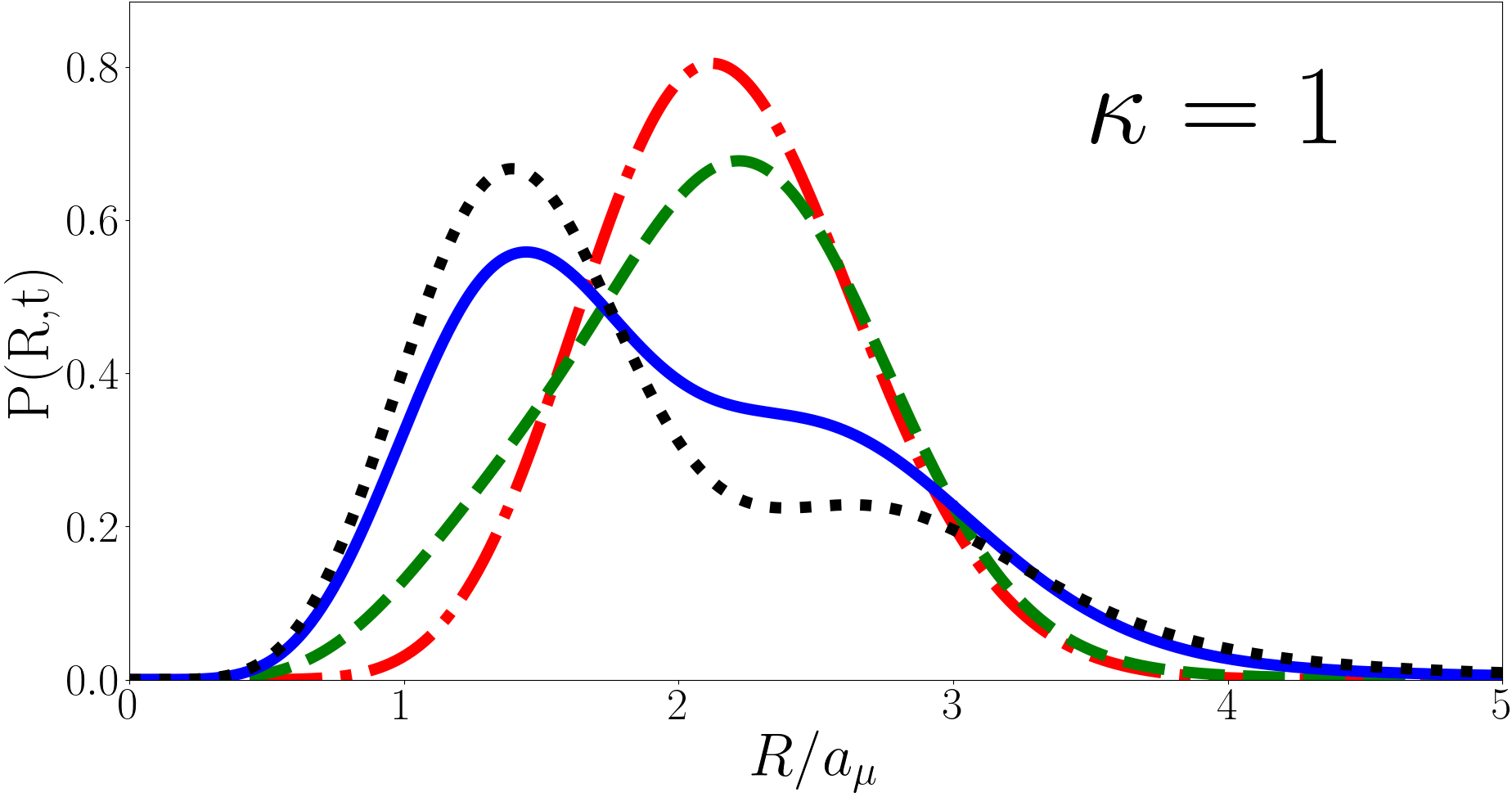
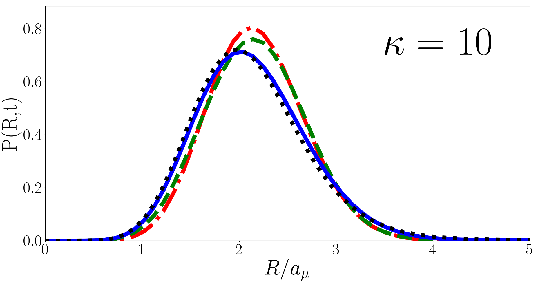
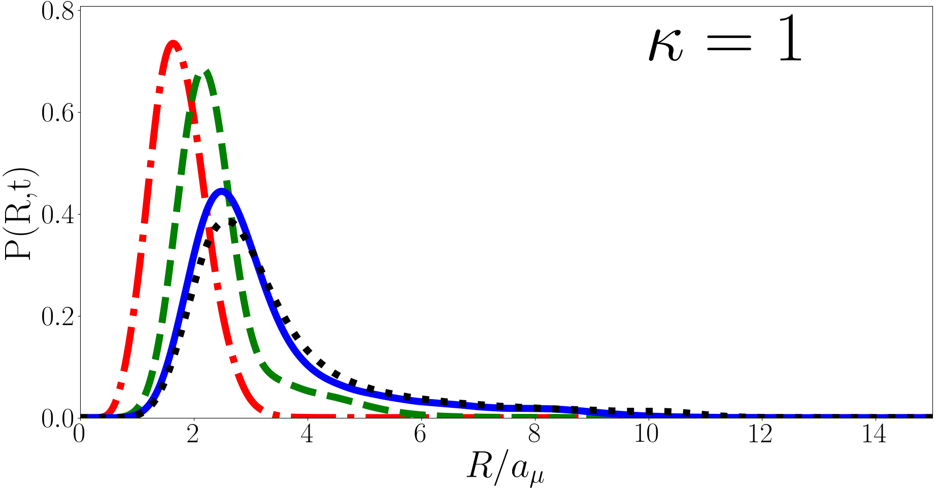
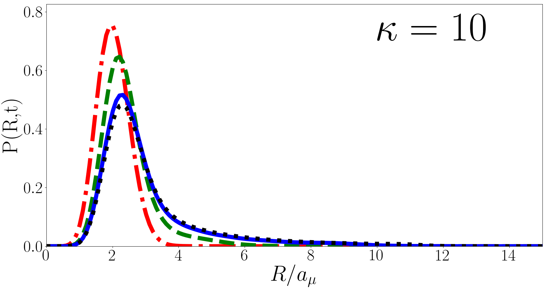
In Fig. 5 we plot $P(R,t)$ at $t=0,0.17\pi/\omega,0.34\pi/\omega$, and $\pi/\omega$ for $\kappa=0.1,1$, and $10$ (heavy impurity, equal mass, and light impurity respectively) as a function of $R$ for the forwards quench. We find that the peak of the probability distribution shifts inwards as the system evolves, reaching its innermost point at $t=\pi/2\omega$ then evolving in reverse back to its original configuration and continuing to oscillate in this way with period $t=\pi/\omega$. The magnitude of oscillation is smaller for larger $\kappa$. This oscillatory behaviour and its dependence on $\kappa$ is unsurprising given the behaviour observed in Fig. 3. However the double peak, which is present for $\kappa\lesssim 5$, is unusual. We can illuminate the double peak structure by looking at the overlaps of the pre- and post-quench wavefunctions. Looking at the $\kappa=0.1$ (heavy impurity) case the largest overlaps are $|\bra{F_{0,4}\phi_{0,4}}\ket{F_{0,2.004}\phi_{0,2.004}}|^{2}\approx 0.539$, $|\bra{F_{0,4}\phi_{0,4}}\ket{F_{0,5.817}\phi_{0,5.817}}|^{2}\approx 0.134$ and $|\bra{F_{0,4}\phi_{0,4}}\ket{F_{1,2.004}\phi_{0,2.004}}|^{2}\approx 0.179$. $\langle\tilde{R}\rangle$ of these states projected onto are $\approx 1.66$, $\approx 2.56$, and $\approx 2.07$ respectively. Compare this to the $\kappa=10$ (light impurity) case where the most significant states are $|\bra{F_{0,4}\phi_{0,4}}\ket{F_{0,3.3169}\phi_{0,3.3169}}|^{2}\approx 0.607$, and $|\bra{F_{0,4}\phi_{0,4}}\ket{F_{0,4.707}\phi_{0,4.707}}|^{2}\approx 0.350$ and $\langle\tilde{R}\rangle$ of the states projected onto are $\approx 2.01$ and $\approx 2.33$. For small $\kappa$ the initial state most heavily overlaps with a few states with a relatively large variation in $\langle\tilde{R}\rangle$ for large $\kappa$ the overlaps are with states that are more closely clustered in $\langle\tilde{R}\rangle$ hence $P(R,t=\pi/2\omega)$ is singly peaked in the latter case. Physically speaking the oscillation amplitude grows smaller for a lighter impurity particle because the less mass (and therefore momenta) it has the less it is able to affect the positions of the two fermions. For the forwards quench we find $P(R,t)$ is convergent as $N_{\rm max}\rightarrow\infty$ at all points in time, as expected given $\langle R(t)\rangle$ is convergent for the forwards quench. We now turn to the divergent case, the reverse quench.

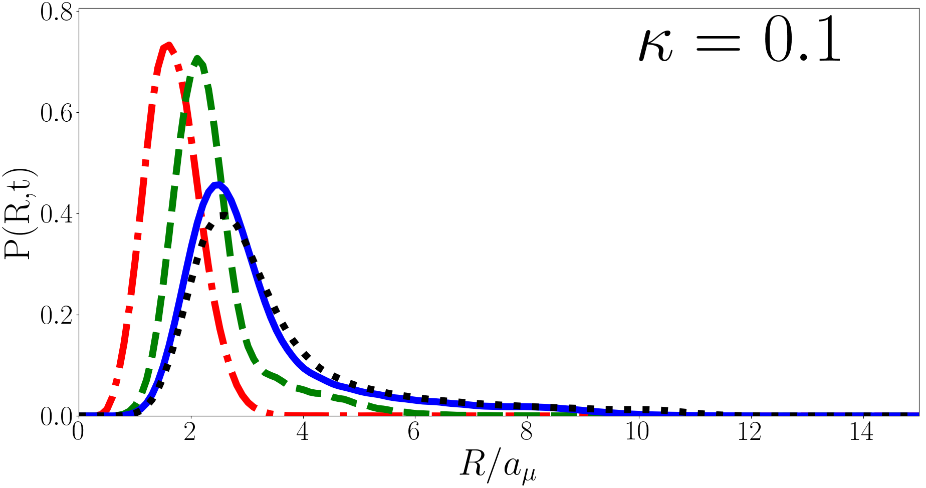
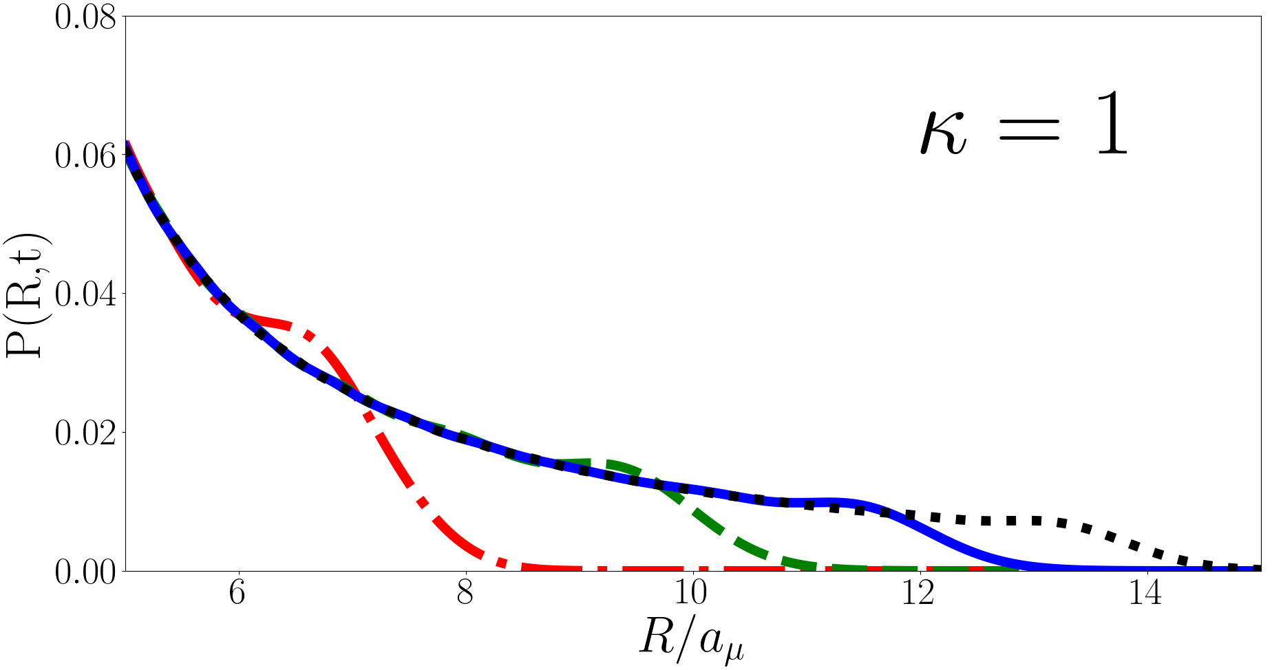
In Fig. 6 we plot $P(R,t)$ at $t=0,0.17\pi/\omega,0.34\pi/\omega$, and $\pi/\omega$ for $\kappa=0.1,1$, and $10$ (heavy impurity, equal mass, and light impurity respectively) as a function of $R$ for the backwards quench. As with the forwards quench $P(R,t)$ oscillates with period $\pi/\omega$ however the peak initially moves outwards rather than inwards. The magnitude of the oscillations grows smaller for larger $\kappa$ (lighter impurity) but the behaviour is qualitatively similar whatever the mass imbalance. For $t=n\pi/\omega$ $P(R,t)$ is approximately a Gaussian and converges with $N_{\rm max}$, however away from $t=n\pi/\omega$ the probability distribution develops a long tail. The behaviour of the tail at $t=\pi/2\omega$ for $\kappa=1$ is plotted in Fig. 7 for various $N_{\rm max}$ and the behaviour is qualitatively similar for different $\kappa$. The long tail decays approximately as $1/\tilde{R}^{2}$ before becoming exponentially suppressed, a “cut-off”. The larger $N_{\rm max}$ is the later the cut-off occurs. While $P(R,t=\pi/2\omega)$ is normalised as $N_{\rm max}\rightarrow\infty$ this increasing long tail means that integral of $RP(R,t=\pi/2\omega)$ from $R=0$ to $R\rightarrow\infty$ is divergent, hence $\langle\tilde{R}\rangle$ diverges.

In the two-body case it has been suggested that the divergence in $\langle r\rangle=\langle|\vec{r}_{1}-\vec{r}_{2}|\rangle$ is due to the $1/r$ divergence in the two-body relative wavefunctionKerin and Martin (2020). In the three-body case the hyperradial part of Eq. (8) does not have a $1/R$ divergence and has a cusp at $\tilde{R}\rightarrow 0$ for the unitary $\kappa=0.1$ (heavy impurity) and $\kappa=1$ (equal mass) ground states but not for the $\kappa=10$ (light impurity) ground state. Nonetheless the divergence in $\langle\tilde{R}(t)\rangle$ is present in all three cases. More specifically we find that for $s_{\rm i}<3$ the initial wavefunction exhibits a cusp, whilst for $s_{\rm i}\geq 3$ there is no cusp in the initial wavefunction. Regardless of which regime the initial state is in the logarithmic divergence of $\langle\tilde{R}(t)\rangle$ persists.

However, it is clear that the finite range of the interaction in a real system provides a natural cut-off in the sum in Eq. (28). A finite range of interaction defines a minimum de Broglie wavelength which in turn defines a maximum energy which defines a maximum number of terms in the sums of Eq. (28) and thus a maximum $\langle\tilde{R}(t)\rangle$. For a system of three sodium atoms (i.e. $\kappa=1$) in a 1kHz trap and an interaction cut-off of $10^{-9}$m we obtain a cut off energy of $E_{\rm rel}\approx 8.7\times 10^{6}\hbar\omega$ and thus expect a maximum $\langle\tilde{R}(t)\rangle$ of $\approx 11$. With this cut-off $\langle\tilde{R}(t)\rangle$ for the backwards quench oscillates between $\approx 1.5$ and $\approx 11$, an amplitude of $\approx 5$. This is significantly larger than in the forwards quench where $\langle\tilde{R}(t)\rangle$ oscillates between $\approx 1.8$ and $\approx 2.2$. In light of the divergence it is natural to consider the effect of using finite-range interaction models rather than zero-range as done here, and the case of two-bodies with a soft-core interaction has been solved analytically in a one-dimensional harmonic trap Kościk and Sowiński (2018). In the limit of small interaction range it is likely that the dynamics will be similar, but the effects of longer range interactions on the dynamics are unclear. If the source of the $\langle\tilde{R}(t)\rangle$ divergence is indeed the zero-range nature of the interaction then the finite-range model may not have the divergence present in the zero-range model.

However the zero-range interaction is not the only non-physical aspect of this model. We assume that the quench in $a_{\rm s}$ is instantaneous, in experiment $a_{\rm s}$ will change continuously over some finite time. The instantaneous quench we consider here may also be related to the $\langle\tilde{R}(t)\rangle$ divergence in the backwards quench, but it is difficult to calculate a non-instantaneous quench in this formalism. In the two-body formalism it is possible to quench between any two scattering lengths Kerin and Martin (2020) and thus numerically calculate a non-instantaneous quench. It would be interesting to see how this would affect the dynamics of the system and if this affects the divergence.

References

- Serwane et al. (2011) F. Serwane, G. Zürn, T. Lompe, T. Ottenstein, A. Wenz, and S. Jochim, Science 332, 336 (2011).
- Murmann et al. (2015) S. Murmann, A. Bergschneider, V. M. Klinkhamer, G. Zürn, T. Lompe, and S. Jochim, Physical Review Letters 114, 080402 (2015).
- Zürn et al. (2013) G. Zürn, A. N. Wenz, S. Murmann, A. Bergschneider, T. Lompe, and S. Jochim, Physical Review Letters 111, 175302 (2013).
- Zürn et al. (2012) G. Zürn, F. Serwane, T. Lompe, A. N. Wenz, M. G. Ries, J. E. Bohn, and S. Jochim, Physical Review Letters 108, 075303 (2012).
- Stöferle et al. (2006) T. Stöferle, H. Moritz, K. Günter, M. Köhl, and T. Esslinger, Physical Review Letters 96, 030401 (2006).
- Cui (2012) X. Cui, Few Body Systems 52, 65 (2012).
- D’Incao et al. (2018) J. P. D’Incao, J. Wang, and V. Colussi, Physical Review Letters 121, 023401 (2018).
- Jonsell et al. (2002) S. Jonsell, H. Heiselberg, and C. Pethick, Physical Review Letters 89, 250401 (2002).
- Blume and Daily (2010) D. Blume and K. M. Daily, Physical review letters 105, 170403 (2010).
- Kerin and Martin (2022) A. Kerin and A. Martin, arXiv preprint arXiv:2204.09205 (2022).
- Kestner and Duan (2007) J. Kestner and L.-M. Duan, Physical Review A 76, 033611 (2007).
- Liu et al. (2009) X.-J. Liu, H. Hu, and P. D. Drummond, Physical Review Letters 102, 160401 (2009).
- Liu et al. (2010) X.-J. Liu, H. Hu, and P. D. Drummond, Physical Review A 82, 023619 (2010).
- Rakshit et al. (2012) D. Rakshit, K. M. Daily, and D. Blume, Physical Review A 85, 033634 (2012).
- Kaplan and Sun (2011) D. B. Kaplan and S. Sun, Physical Review Letters 107, 030601 (2011).
- Mulkerin et al. (2012a) B. Mulkerin, C. Bradly, H. Quiney, and A. Martin, Physical Review A 85, 053636 (2012a).
- Mulkerin et al. (2012b) B. C. Mulkerin, C. J. Bradly, H. M. Quiney, and A. M. Martin, Physical Review A 86, 053631 (2012b).
- Nascimbène et al. (2010) S. Nascimbène, N. Navon, F. Jiang, K. Chevy, and C. Salomon, Nature 463, 1057 (2010).
- Ku et al. (2012) M. Ku, A. Sommer, L. Cheuk, and M. Zwierlein, Science 335, 563 (2012).
- Levinsen et al. (2017) J. Levinsen, P. Massignan, S. Endo, and M. M. Parish, Journal of Physics B: Atomic, Molecular and Optical Physics 50, 072001 (2017).
- Daily and Blume (2010) K. Daily and D. Blume, Physical Review A 81, 053615 (2010).
- Colussi et al. (2018) V. Colussi, J. P. Corson, and J. P. D’Incao, Physical review letters 120, 100401 (2018).
- Colussi et al. (2019) V. Colussi, B. van Zwol, J. D’Incao, and S. Kokkelmans, Physical Review A 99, 043604 (2019).
- Enss et al. (2022) T. Enss, N. C. Braatz, and G. Gori, arXiv preprint arXiv:2203.06098 (2022).
- Bougas et al. (2022) G. Bougas, S. Mistakidis, P. Giannakeas, and P. Schmelcher, arXiv preprint arXiv:2205.02015 (2022).
- Pecak et al. (2016) D. Pecak, M. Gajda, and T. Sowiński, New Journal of Physics 18, 013030 (2016).
- Volosniev (2017) A. G. Volosniev, Few-Body Systems 58, 1 (2017).
- Kehrberger et al. (2018) L. M. A. Kehrberger, V. J. Bolsinger, and P. Schmelcher, Physical Review A 97, 013606 (2018).
- Sowiński and García-March (2019) T. Sowiński and M. Á. García-March, Reports on Progress in Physics 82, 104401 (2019).
- Kerin and Martin (2020) A. D. Kerin and A. M. Martin, Physical Review A 102, 023311 (2020).
- Werner and Castin (2006a) F. Werner and Y. Castin, Physical Review Letters 97, 150401 (2006a).
- Werner (2008) F. Werner, Theses, Université Pierre et Marie Curieâ Paris VI, Paris France (2008).
- Werner and Castin (2006b) F. Werner and Y. Castin, Physical Review A 74, 053604 (2006b).
- Bethe and Peierls (1935) H. Bethe and R. Peierls, Proceedings of the Royal Society of London. Series A-Mathematical and Physical Sciences 148, 146 (1935).
- Srivastava et al. (2003) H. M. Srivastava, H. A. Mavromatis, and R. S. Alassar, Applied Mathematics Letters 16, 1131 (2003).
- Nielsen et al. (2001) E. Nielsen, D. V. Fedorov, A. S. Jensen, and E. Garrido, Physics Reports 347, 373 (2001).
- Fedorov and Jensen (1993) D. Fedorov and A. Jensen, Physical review letters 71, 4103 (1993).
- Fedorov and Jensen (2001) D. V. Fedorov and A. Jensen, Journal of Physics A: Mathematical and General 34, 6003 (2001).
- Braaten and Hammer (2006) E. Braaten and H.-W. Hammer, Physics Reports 428, 259 (2006).
- Thøgersen (2009) M. Thøgersen, arXiv preprint arXiv:0908.0852 (2009).
- Colussi (2019) V. E. Colussi, Atoms 7, 19 (2019).
- Kościk and Sowiński (2018) P. Kościk and T. Sowiński, Scientific Reports 8, 1 (2018).
- Fano (1935) U. Fano, Il Nuovo Cimento 12, 154 (1935).
- Feshbach (1958) H. Feshbach, Annals of Physics 5, 357 (1958).
- Tiesinga et al. (1993) E. Tiesinga, B. J. Verhaar, and H. T. C. Stoof, Physical Review A 47, 4114 (1993).
- Chin et al. (2010) C. Chin, R. Grimm, P. Julienne, and E. Tiesinga, Reviews of Modern Physics 82, 1225 (2010).
- Cetina et al. (2016) M. Cetina, M. Jag, R. S. Lous, I. Fritsche, J. T. Walraven, R. Grimm, J. Levinsen, M. M. Parish, R. Schmidt, M. Knap, et al., Science 354, 96 (2016).
- Guan et al. (2019) Q. Guan, V. Klinkhamer, R. Klemt, J. H. Becher, A. Bergschneider, P. M. Preiss, S. Jochim, and D. Blume, Physical Review Letters 122, 083401 (2019).
- Endo and Castin (2015) S. Endo and Y. Castin, Physical Review A 92, 053624 (2015).
- Castin et al. (2010) Y. Castin, C. Mora, and L. Pricoupenko, Physical review letters 105, 223201 (2010).