Quiver algebras as Fukaya categories
Abstract.
We embed triangulated categories defined by quivers with potential arising from ideal triangulations of marked bordered surfaces into Fukaya categories of quasi-projective 3-folds associated to meromorphic quadratic differentials. Together with previous results, this yields non-trivial computations of spaces of stability conditions on Fukaya categories of symplectic six-manifolds.
1. Introduction
A marked bordered surface comprises a compact, connected oriented surface , perhaps with non-empty boundary, together with a non-empty set of marked points, such that every boundary component of contains at least one marked point. We always assume that is not a sphere with fewer than five marked points. An ideal triangulation of gives rise, via work of Labardini-Fragoso [32], to a quiver with potential. The CY3 -triangulated category of finite-dimensional modules over the corresponding Ginzburg algebra depends only on the underlying data . This paper embeds these categories, under mild hypotheses on , into Fukaya categories of quasi-projective 3-folds. The 3-folds are the total spaces of affine conic fibrations over ; whilst these spaces have not appeared previously in the literature, they are close cousins of those studied in [8]. Together with the main results of [5], we therefore obtain computations of spaces of stability conditions on (distinguished subcategories of) Fukaya categories of symplectic six-manifolds.
We work over an algebraically closed field of characteristic zero. For much of the paper, we take to be the single variable Novikov field (with formal parameter ),
| (1.1) |
which is algebraically closed by [15, Lemma 13.1].
1.1. Surfaces and differentials
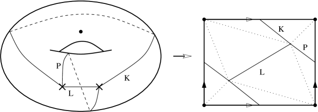
Let be a marked bordered surface. An ideal triangulation of with vertices at has an associated quiver with potential , which can be defined over any algebraically closed field . The construction is indicated schematically in the case where is non-degenerate in Figure 1 and Equation (2.2), and defined more generally in [32]. There is a triangulated CY3 category of finite type (i.e. cohomologically finite) over defined by the Ginzburg algebra construction [19]; this has a distinguished heart, equivalent to the category of finite-dimensional modules for the complete Jacobi algebra of the quiver with potential . Results of Keller-Yang and Labardini-Fragoso imply that depends up to quasi-isomorphism only on the underlying marked bordered surface . We write for any category in this equivalence class.
A meromorphic quadratic differential on a Riemann surface has an associated marked bordered surface . The surface is obtained as the real blow-up of at poles of of order ; the distinguished tangent directions of the horizontal foliation of define boundary marked points in , and poles of order define the punctures (interior marked points) . We will write for the set of poles, and , for poles of constrained or specified orders. For let denote the order of the corresponding pole.
All quadratic differentials considered in this paper have simple zeroes.
Let denote the complex orbifold parametrizing equivalence classes of pairs comprising a Riemann surface and a meromorphic quadratic differential with simple zeroes whose associated marked bordered surface is diffeomorphic to . This has an open dense subset of pairs where the differential has poles of order exactly at , or equivalently for which the flat metric defined by is complete. There is an unramified cover whose points are signed meromorphic differentials, meaning that we fix a choice of sign of the residue of the differential at each double pole; the cover extends as a ramified cover .
1.2. The threefolds
Fix a signed complete differential . Denote by the divisor on , where denotes the smallest integer greater than or equal to , and write
| (1.2) |
corresponding to the obvious decomposition . Take a rank two holomorphic vector bundle on with . We perform an elementary modification of the vector bundle at each double pole of , to obtain a rank three bundle fitting into a short exact sequence
We then remove from all poles of of order .
The determinant map restricts to a quadratic map on the bundle which is rank one at points of . The threefold
is an affine conic fibration over , with nodal fibres over the zeroes of , fibres singular at infinity over the double poles, and empty fibres over higher order poles. The topology of the fibre over a double pole depends on the choice of elementary modification. A choice of line in the fibre of at determines a distinguished elementary modification, with the property that the resulting fibre of at is isomorphic to the disjoint union of two planes . We will always consider elementary modifications with this property.
1.3. The result
We fix a linear Kähler form on . This induces a Kähler form on . A Moser-type argument, see Lemma 3.17, shows that (having fixed the parameters determining the cohomology class of the Kähler form appropriately) the symplectic manifold underlying depends up to isomorphism only on the pair . has vanishing first Chern class, and determines a distinguished homotopy class of trivialisation of the canonical bundle of .
When , the Kähler form is exact, and has a well-defined exact Fukaya category , which may be constructed over any field , see [47]. More generally, we will consider Lagrangian submanifolds with the following property: there is an almost complex structure on , taming the symplectic form and co-inciding with the given integrable structure at infinity, for which bounds no -holomorphic disk and does not meet any -holomorphic sphere. For ease of notation, we will refer to such as strictly unobstructed. When is closed, has a strictly unobstructed Fukaya category (which we again denote by) , now defined over the Novikov field . This version of the Fukaya category appears, for instance, in [2] and [49]. The strictly unobstructed hypothesis rules out bubbling of holomorphic disks, which simplifies the technical construction of , see [49, Sections 3b, 3c] for a detailed discussion under slightly weaker hypotheses.
Let be a symplectic manifold with well-defined Fukaya category . For each , there is a category , the -twisted strictly unobstructed Fukaya category, which for recovers the category considered previously. Objects of are closed oriented graded strictly unobstructed Lagrangians , which are equipped with a relative spin structure111In other words, and we fix a trivialisation of over the 2-skeleton of , where is the unique real 2-plane bundle with and ., relative to the background class . The choice of background class serves to change the signs with which holomorphic polygons contribute to the -operations , and can be seen as fixing a particular coherent orientation scheme for the Fukaya category; compare to [47, Section 11 & Remark 12.1].
Each category is a -graded -category, linear over the appropriate field . Let denote the cohomological category of the category of twisted complexes over an -category .
Now consider the threefold . For each , the fibre is reducible. Let denote one component of this fibre. We fix the background class represented by the locally finite cycle
| (1.3) |
given by (either) one of the components of the reducible fibre at each point of , or equivalently each point of . The class is non-trivial by Lemma 3.11. Different choices of cycle representative for are related by monodromy by Lemma 3.12.
Theorem 1.1.
Let be a marked bordered surface, with . Suppose either
-
(1)
is closed, , , and ; or
-
(2)
, and is not a sphere with fewer than five punctures.
There is a -linear fully faithful embedding
The untwisted Fukaya category , which differs from by certain signs, is different, and is discussed in Section 5.4.
One drawback of Theorem 1.1 is that it does not give a symplectic characterisation of the image of the embedding . There is an obvious candidate for such a characterisation, which we now explain.
Any embedded path , with end-points distinct zeroes of and otherwise disjoint from the zeroes and poles of , defines a Lagrangian 3-sphere , fibred over the arc via Donaldson’s “matching cycle” construction [47, III, Section 16g]. The matching spheres are exact if and strictly unobstructed (with the canonical complex structure on ) when is closed and . A Lagrangian sphere is relatively spin for any choice of background class , hence equipped with a grading defines a Lagrangian brane in . A non-degenerate ideal triangulation of defines a full subcategory , generated by the matching spheres associated to the edges of the cellulation dual to . Theorem 1.1 is proved by showing that for particularly well-behaved triangulations . Since the category does not depend on , it follows that also depends only on the pair , up to triangulated equivalence.
Let be the full -subcategory generated by Lagrangian matching spheres. This manifestly depends only on the pair . It seems likely that . We outline one tentative approach to proving that, which amounts to proving that generates , in Section 4.9, but elaborating the details of that sketch would be a substantial task. Going further, it seems likely that all Lagrangian spheres in are quasi-isomorphic to matching spheres (the result is proved in special cases in [2, 50]), in which case the category would be a symplectic invariant of , carrying an action of the subgroup of preserving the class . The question of whether the embedding itself split-generates is also open, though here there seems to be less evidence either way. We hope to return to these questions elsewhere.
The imposed condition gives a substantial simplication since holomorphic polygons are constrained for grading considerations that do not pertain when is globally holomorphic, cf. Remarks 3.22 and 4.15. The constraint on the number of punctures when is closed arises from a similar constraint in work of Geiss, Labardini-Fragoso and Schröer [18], who study the action of right equivalences on potentials on the quivers , cf. Theorem 2.1. We conjecture that, for a closed surface of genus , Theorem 1.1 holds under the weaker hypothesis . (Once-punctured surfaces are special: not every pair of signed ideal triangulations are related by pops and flips, and when the analogue of Theorem 2.1 is actually false, cf. [18].)
One can relax the strict unobstructedness hypothesis at the cost of invoking the deep obstruction theory of [14] in the construction of . If is closed and then may contain rational curves, so only the more complicated construction is available. This is the reason for the genus constraint in the first part of Theorem 1.1.
Remark 1.2.
The elementary modifications appearing in the specific construction of play a definite role in reproducing , which seems somewhat less natural from the viewpoint of the symplectic topology of the original bordered surface , not least because of the CY3 property. The particular choice of elementary modification that we employ was motivated by two considerations: first, to yield the Calabi-Yau property of Lemma 3.5, and second, to ensure the non-vanishing of a certain count of local holomorphic sections over discs centred on double poles in Lemma 4.10. (The latter result would fail if instead one took the threefold to have smooth, nodal, higher multiplicity or empty fibres over the double poles, and also accounts for the appearance of the twisting class .) At a more technical level, the appearance of a reducible fibre whose components are exchanged by the local monodromy of the family of threefolds obtained by allowing the residue at a double pole to wind once around the origin, cf. Lemma 3.12, fits well with the appearance of “signed” quadratic differentials in [5, Section 6.2].
1.4. Context
In many cases, the paper [5] computes the space of stability conditions on the category in terms of moduli spaces of quadratic differentials. If either is closed with and with at least two punctures, or and is not a sphere with fewer than six punctures, there is a connected component of and a subgroup of autoequivalences which preserve this component modulo those which act trivially upon it, with
where has the same coarse moduli space as but additional orbifolding along the incomplete locus, see [5] for details. This gives a non-trivial computation of the space of stability conditions on (a subcategory of) the Fukaya category of a symplectic six-manifold, and enables one to understand the Donaldson-Thomas invariants of these categories.
One can construct a complex (3,0)-form on with the following property: if the path is a saddle connection for , the associated matching sphere is special, i.e. has constant phase on . (We are not working with the Ricci-flat metric, so these are not strictly special in the traditional sense.) There are similarly -special Lagrangian submanifolds of associated to homotopically non-trivial closed geodesics for the flat metric defined by . Theorem 1.4 of [5] implies that the Donaldson-Thomas invariants of , defined with respect to the stability condition associated to , count such special Lagrangian submanifolds, the existence and numerics of which are therefore governed by the Joyce-Song and Kontsevich-Soibelman wall-crossing formulae [24, 30]. This confirms, in this special case, a long-standing expectation of Joyce and others.
It is natural to conjecture that moduli spaces of holomorphic quadratic differentials with simple zeroes arise as spaces of stability conditions (modulo autoequivalences) on the Fukaya categories of the local threefolds of [8] (see Equation 3.1). However, these categories do not appear to admit descriptions in terms of quivers, and different techniques would be required to analyse them and the corresponding spaces of stability conditions.
1.5. Higher rank
The threefolds are associated to meromorphic maps of Riemann surfaces into the versal deformation space of the -surface singularity . There are also local threefolds associated to meromorphic maps to the versal deformation spaces of other ADE singularities: in the case of a holomorphic map, the relevant threefolds are studied in [8, 55]. Already for the -surface, however, the geometry is substantially more complicated, and the relationship to stability conditions rather less clear.
The natural data required to write down a quasi-projective Calabi-Yau threefold fibred over a Riemann surface in the -case is a tuple comprising (perhaps meromorphic) sections of for . For instance, when and supposing one is working with holomorphic rather than meromorphic differentials, one takes a vector bundle with , and considers the hypersurface
| (1.4) |
where and . For generic choices of this is a smooth Calabi-Yau, the total space of a Lefschetz fibration over , with generic fibre the Milnor fibre of (symplectically, the plumbing of two copies of ).
However, the moduli space of such data – a complex structure on and a tuple of differentials – has dimension smaller than the dimension of the space of stability conditions on the corresponding category, or more mundanely smaller than the rank of of the associated threefold (compare to Remark 3.15). This is a familiar problem: whilst one expects spaces of complex structures on a symplectic Calabi-Yau to embed into the space of stability conditions on the Fukaya category, there is no reason to expect that embedding to be onto an open subset. The fortunate accident in the -case is that Teichmüller space has the same dimension as the space of quadratic differentials. At least for -fibred threefolds, it seems natural following [33] to expect the “higher Teichmüller space”, i.e. Hitchin’s contractible component [22] of the variety of flat -connections, to play a role in resolving this discrepancy.
Finally, we note that computations in [17] indicate that the CY3 -categories arising in higher rank (even when one restricts to meromorphic differentials) are appreciably more complicated; whereas the Donaldson-Thomas invariants of the categories studied in this paper are always or , cf. [5], and non-vanishing only for primitive classes, in the higher rank case one expects there are classes for which the DT-invariants (conjecturally related to counts of special Lagrangian submanifolds in the corresponding threefold) in class grow exponentially with . The symplectic topology of (1.4) is the subject of work in progress by the author.
1.6. Standing assumptions
The arguments for the two cases of Theorem 1.1 are rather similar. For definiteness, for the rest of the paper we consider the (more complicated) case when is closed, leaving the required modifications for the case with non-empty boundary to the interested reader.
In the closed case all the marked points are punctures. To avoid transversality issues arising from rational curves and their multiple covers, we also exclude the (interesting) case of threefolds fibring over the 2-sphere. Therefore the discrete topological data will henceforth be indexed by a pair with and .
Acknowledgements. Tom Bridgeland was originally to be a co-author; his influence is pervasive. I am indebted to Daniel Labardini-Fragoso for explanations of his joint work with Geiss and Schröer [18], on which we rely essentially. Thanks also to Mohammed Abouzaid, Bernhard Keller, Yankl Lekili, Andy Neitzke, Oscar Randal-Williams, Tony Scholl, Paul Seidel, Balazs Szendroi and Richard Thomas for helpful conversations; Abouzaid and Seidel provided assistance with a crucial sign computation. Finally, I am grateful to the anonymous referee for suggesting many improvements to the exposition.
2. Background
2.1. Quivers with potential
Let be a quiver, specified by sets of vertices and arrows , , and source and target maps . We write for the path algebra of over the field , and for the completion of with respect to path length. A potential on is an element of the closure of the subspace of spanned by all cyclic paths in of length . A potential is called reduced if it lies in the closure of the subspace spanned by cycles of length .
We say that two potentials and are cyclically equivalent if lies in the closure of the subspace generated by differences , where is a cycle in the path algebra. and are right-equivalent if there is an automorphism of the completed path algebra which fixes the zero-length paths and such that and are cyclically equivalent. Following [18], we say and are weakly right equivalent if and are right-equivalent, for some invertible scalar .
Consider minimal categories whose objects are indexed by the vertices of , and such that, as a graded vector space
where is the space with basis consisting of arrows in connecting vertex to vertex . There is an obvious non-degenerate pairing
Thus, if we define
an product of degree ,
is equivalently described by a linear map of degree
| (2.1) |
Let us insist that is cyclic as an category, meaning that the tensors are cyclically invariant in the graded sense. If we further insist that the structure on is strictly unital then the whole structure is determined by the elements when all the have degree 1. For background on this construction, see [43].
Let be a reduced potential on . Decomposing the potential into homogeneous pieces, and cyclically symmetrising, we obtain linear maps
Setting gives a well-defined category . Define to be the homotopy category of the category of twisted complexes over
The associated graded category of contains as a full subcategory.
The same category admits an alternative (Koszul dual) description in terms of the derived category of a dg algebra called the complete Ginzburg algebra (see for instance [30, Theorem 9] or [26, Section 5]). To define it, first double , adding a dual edge for each , and then add loops based at each vertex of . The resulting quiver has a grading given by
Let be the completion of the path algebra as a graded algebra, with respect to the ideal generated by the arrows of . There is a unique continuous differential satisfying
Thus is a dg algebra. The category can then be equivalently described as the full subcategory of the derived category of the dg algebra consisting of finite-dimensional modules. By a general result of Keller and Van den Bergh [27], this description shows that is a CY3 triangulated category.
Keller and Yang [28, Lemma 2.9] showed that if and are right-equivalent potentials, they have isomorphic complete Ginzburg algebras, and hence yield equivalent categories . Ladkani [34, Proposition 2.7], see also [18, Lemma 8.5], showed that the same conclusion holds when and are only weakly right-equivalent. Indeed, there is a natural -action on the set of minimal -structures on the category , where acts by rescaling the operation by . -structures related by the -action are -equivalent even though not gauge-equivalent in the usual sense (the required equivalence does not act by the identity on cohomology but by a multiple of the Euler vector field). The potentials and on give rise to -categories and which are related by the -action. Since -equivalences induce equivalences on categories of twisted complexes by [47, Lemma 3.20], the category depends only on the weak right equivalence class of .
The fact that is concentrated in non-positive degrees implies [28, Lemma 5.2] that is equipped with a canonical bounded t-structure, whose heart is equivalent to the category of nilpotent representations of the completed Jacobian algebra
In particular, is a finite-length heart. Since it admits a bounded t-structure, the category is split-closed, i.e. agrees with its own idempotent completion, see [35].
2.2. Quivers from triangulated surfaces
Suppose again that is a closed oriented surface of genus , now equipped with a non-empty set of marked points .
By a non-degenerate ideal triangulation of we mean a triangulation of whose vertex set is precisely , and in which every vertex has valency at least (this implies that every triangle has three distinct edges). A signed triangulation is a triangulation equipped with a function
We can associate a quiver with potential to a signed non-degenerate triangulation as follows.
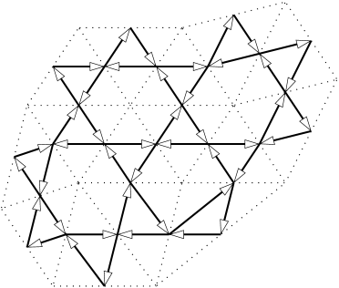
The quiver has vertices at the midpoints of the edges of , and is obtained by inscribing a small clockwise 3-cycle inside each face of , as in Figure 1. There are two obvious systems of cycles in , namely a clockwise 3-cycle in each face , and an anticlockwise cycle of length at least 3 encircling each point . Define a potential
| (2.2) |
When we will sometimes omit it from the notation.
Consider the derived category of the completed Ginzburg algebra of the quiver with potential over , and let be the full subcategory consisting of modules with finite-dimensional cohomology. As a special case of the discussion of Section 2.1, this is a CY3 triangulated category of finite type over , and comes equipped with a canonical t-structure, whose heart is equivalent to the category of finite-dimensional modules for the completed Jacobi algebra of .
Suppose two non-degenerate ideal triangulations are related by a flip, in which the diagonal of a quadilateral is replaced by its opposite diagonal. The resulting quivers with potential (in which the signing is unchanged) are related by a mutation at the vertex corresponding to the edge being flipped. It follows from general results of Keller and Yang [28] that there exist distinguished -linear triangulated equivalences .
Labardini-Fragoso [32] extended the above definitions so as to encompass a larger class of signed ideal triangulations (ones containing self-folded triangles, in which two of the three edges co-incide; in this case there may be punctures of valency one, and the mutation operation can change the signing). He moreover proved that flips also induce right-equivalences in this more general context. There is another operation on signed ideal triangulations, which involves changing the signing at a given puncture without changing the triangulation, and a corresponding “pop” equivalence which relates the associated categories. Under our hypothesis on that , any two of these more general signed ideal triangulations are related by a finite chain of flips and pops. It follows that up to -linear triangulated equivalence, the category is independent of the chosen triangulation and of the choice of signing; see [5, Sections 8 & 9] for a more detailed discussion. We denote by any triangulated category in this quasi-equivalence class.
Given the quiver , one can define a CY3 category by taking any potential on , not necessarily the potential described above. We will say that two potentials and are disjoint if no cycle occuring in is cyclically equivalent to a cycle appearing in . The following result is due to Geiss, Labardini-Fragoso and Schröer [18].
Theorem 2.1.
Let be a triangulation of which contains no self-folded triangles or loops and in which every vertex has valency at least 4. Suppose that the associated quiver contains no double arrows. Any two potentials on of the form
| (2.3) |
(for scalars and disjoint from the and ) are weakly right equivalent.
Geiss, Labardini-Fragoso and Schröer furthermore prove that every pair with and with admits some triangulation which satisfies the hypotheses, i.e. which contains no self-folded triangle or loop, in which every vertex has valency at least 4, and for which the associated quiver has no double arrow. (In the case when has non-empty boundary, the same result holds without further hypotheses on the number of punctures.) The proof of Theorem 2.1 involves a delicate, iterative construction of a suitable right-equivalence by hand, obtained as an infinite composition of equivalences which, to first approximation, increase the minimal length of any cycle appearing in the remainder term ; the actual proof is more complicated than this suggests.
For our purposes, these results yield a finite-determinacy theorem for -structures on the total endomorphism algebra of the category of Section 2.1 in the special case . Considering the description of the category as a category of twisted complexes over an -algebra given in Section 2.1, Theorem 2.1 implies in particular that different choices of scalars for the potential (2.3) yield equivalent categories , whilst -products encoded by the “remainder” term can be gauged away.
2.3. Quadratic differentials and flat metrics
Let denote a pair comprising a Riemann surface and meromorphic quadratic differential with poles of order precisely 2 at the points of a divisor comprising reduced points, and with simple zeroes. Thus, the marked bordered surface associated to is diffeomorphic to . Let denote the set of zeroes, so
At a point of there is a distinguished local co-ordinate with respect to which
This local co-ordinate is uniquely defined up to changes . At simple zeroes, respectively double poles, there is a canonical co-ordinate with respect to which
| (2.4) |
We refer to the value in the second case as the residue at the double pole.
The surface inherits a flat metric with singularities; at each , the metric has a cone angle of . The length element of the metric is defined by
in an arbitrary local parameter , so the length of a curve is given by
This is well-defined for curves passing through zeroes of , but diverges to infinity for curves through double poles. The area of the flat surface
is infinite, since a neighbourhood of each point of is isometric to a semi-infinite flat cylinder of circumference , with as in Equation 2.4.
The differential defines a horizontal foliation of , given by the lines along which . In the natural local co-ordinate, the horizontal foliation is given by lines . The local trajectory structure at a zero shows the horizontal foliation is not transversely orientable. The natural -action by rotation, , does not change the underlying flat surface, but changes which in the circle of foliations defined by is regarded as horizontal.
A saddle connection is a finite length maximal horizontal trajectory. Any such has both end-points at (not necessarily distinct) zeroes of .
2.4. WKB triangulations
Suppose the quadratic differential is complete and saddle-free, meaning that it has no finite-length maximal horizontal trajectory. It then defines a canonical isotopy class of triangulation of with vertices at , called the WKB-triangulation, see [5, Section 10]. There is a dual “Lagrangian cellulation”, with trivalent vertices the zeroes of and which has exactly one face for each point of .
In general, the WKB-triangulation may contain self-folded triangles. Given a quadratic differential whose associated WKB-triangulation contains a self-folded triangle, there is an edge in the Lagrangian cellulation which goes from a zero to itself. The quiver prescription of Labardini-Fragoso differs in this case [32]. For simplicity we will restrict attention to the non-degenerate case:
Lemma 2.2.
For every and there is a complete saddle-free differential whose associated WKB-triangulation contains no self-folded triangles. If one can assume that the triangulation satisfies the further hypotheses of Theorem 2.1. Every edge of the dual cellulation then has distinct end-points.
Proof.
According to [11, Corollary 3.9], any ideal triangulation can be transformed via a sequence of flips to a non-degenerate triangulation (one containing no self-folded triangles), whilst [18] constructs non-degenerate triangulations satisfying the hypotheses of Theorem 2.1 whenever . Any non-degenerate triangulation has an associated bipartite quadrilation , whose vertices are the vertices of together with the mid-points of all faces of , and which has three edges for each face of , which join the vertices of that face to its centre, see Figure 2. Section 4.9 of [5] shows that any quadrilation of the marked surface may be realised as the “horizontal strip decomposition” of a quadratic differential , meaning that has double poles at the vertices of , zeroes at the additional (necessarily trivalent) vertices of , and that the edges of are exactly the trajectories of which contain a zero. It follows that the non-degenerate triangulation obtained in [18] is realised as a WKB triangulation. The final statement is an immediate consequence of non-degeneracy. ∎

For brevity, we will call a triangulation as provided by Lemma 2.2 a non-degenerate WKB triangulation.
3. Threefolds
We now associate quasi-projective Calabi-Yau 3-folds to meromorphic quadratic differentials. By way of motivation, if comprises a Riemann surface of genus and a holomorphic quadratic differential on , there is a quasi-projective 3-fold which is a Lefschetz fibration over , namely
| (3.1) |
This is Calabi-Yau, and its geometry (Abel-Jacobi map, cycle theory etc) have elegant interpretations in terms of geometry on , see [8]. Our spaces are cousins of these, adapted to the case of meromorphic differentials.
3.1. Elementary modification
Let be a closed Riemann surface of genus , equipped with a reduced divisor comprising points. Fix a rank two holomorphic vector bundle
The determinant defines a fibrewise quadratic map
| (3.2) |
Consider an elementary modification of the symmetric square along , fitting into a short exact sequence of sheaves
| (3.3) |
Lemma 3.1.
is locally free of rank , and .
Proof.
The sheaf is torsion-free on a smooth curve, hence locally free. The first Chern class is given by the Whitney sum formula. ∎
Elementary modifications along are not unique, but depend on the choice of in (3.3). It will be important for us to choose the elementary modification compatibly with the quadratic map (3.2).
Lemma 3.2.
There is an elementary modification as above with the property that for each , the induced map
has fibre over any non-zero point of .
Proof.
The statement is obviously local at a given . Let be defined by an equation . Near we fix a trivialisation in which is spanned by holomorphic sections with respect to which the determinant map is given by the fibrewise quadratic
Such a local basis of sections arises naturally from a choice of local basis of sections for near , with , and . The proof of Lemma 3.1 implies there is an elementary modification which is spanned by local holomorphic sections , and the determinant map on is then given by
At , where , the fibre is isomorphic to the disjoint union of two planes , provided . ∎
Note that a choice of complex line in the fibre of at , equivalently of a parabolic structure on at , induces an elementary modification as in Lemma 3.2, where the subspace is identified with the quadratic forms on vanishing on the annihilator of .
3.2. A quasiprojective Calabi-Yau 3-fold
Let be a meromorphic quadratic differential on with simple zeroes and a pole of order exactly at each . Define the hypersurface
inside the total space of the vector bundle . We shall write
for the fibrewise projective completion of . Being fibred in quadrics, this is the zero-locus of a section of , where denotes projection.
The previous description of the determinant map shows that the natural map is a fibration by projective quadrics, with generic fibre , nodal fibres over zeroes of , and reducible fibre at each point of , i.e. the union of two planes joined along a line . The locus of reducible quadrics has codimension in the space of all quadric hypersurfaces in , so a generic one-parameter family of quadrics would have no such singular fibres. The singular fibre is not locally smoothable (i.e. not the -fibre of a smooth three-fold ); an infinitesimal smoothing is determined by a section of the tensor product of the normal bundles to the normal crossing locus in the two components of the singular fibre.
Lemma 3.3.
has two isolated singularities at infinity (i.e. in the complement of ) over each point of , which are 3-fold ordinary double points. These are the only singularities of .
Proof.
Away from , the map is a Lefschetz fibration, and smoothness of the total space is clear. Given the description of the determinant map in Lemma 3.2, a local model for the behaviour near the singular fibres over is given by a neighbourhood of the fibre in the quadric pencil
| (3.4) |
The subspace defines the vector bundle in the given trivialisation, and by hypothesis the holomorphic function vanishes away from . Without loss of generality, we can suppose . Under projection to the second factor , the 0-fibre is which is a union of two planes, whose line of intersection lies in the hyperplane at infinity . The complement of is the affine variety
Under the projection to the plane , this has generic fibre an affine conic , and these degenerate at to a singular fibre . The singularities of the total space of (3.4) are the points
in the given affine charts respectively , which since is locally non-vanishing are both 3-fold ordinary double points. ∎
Corollary 3.4.
is smooth.
Proof.
Removing the section of defining the divisor at infinity removes the line from each reducible fibre, hence removes all the nodes. ∎
The quasi-projective variety comes with a natural projection map .
-
•
The generic fibre of is a smooth affine quadric with , abstractly diffeomorphic to the cotangent bundle ;
-
•
At a zero of , is defined by the quadratic , which has an isolated nodal singularity;
-
•
At a point , recalling that by hypothesis , the fibre is given by an affine quadric , a disjoint union of two planes.
Lemma 3.5.
has holomorphically trivial canonical bundle, hence = 0. The choice of isomorphism defines a canonical homotopy class of trivialisation of the canonical bundle .
Proof.
Consider the -bundle . The determinant map
restricted to is fibrewise quadratic, hence can be viewed as an element of the space of global sections , which pushes forward to give
The projective completion has canonical class . Since
| (3.5) |
and there is an isomorphism , one sees
The quasi-projective subvariety is the complement of the section of at infinity, and the square of that section is a canonical divisor on . The last statement follows from (3.5) since induces . ∎
Lemma 3.6.
There is a nowhere zero holomorphic volume form on .
Proof.
Up to rescaling, there is a unique section of vanishing on the divisor at infinity, and since , the complement admits a canonical holomorphic volume form up to scale. ∎
Remark 3.7.
The form has poles of order 2 at infinity. For a heuristic discussion of the relevance of the pole order being to constructions of stability conditions on the Fukaya category starting from pairs comprising a complex structure and such a non-vanishing volume form, see [31, Section 7.3].
3.3. Resolution
The 3-fold ordinary double point
admits two distinct small resolutions, in which the singular point is replaced by a smooth with normal bundle . The resolutions are obtained by collapsing either one of the two rulings of the exceptional divisor resulting from blowing up the singularity; the passage from one resolution to the other is the simplest example of a 3-fold flop.
Lemma 3.8.
There is a projective small resolution .
Proof.
Let be the total transform of .
Lemma 3.9.
The divisor is smooth, and supports an effective anticanonical divisor.
Proof.
There are two possible models for the singular fibre of over a point of , depending on whether the small resolution curves lie in the same or distinct components of the fibre. Either the generic fibre degenerates to a union of two first Hirzebruch surfaces meeting along a fibre; or it degenerates to a copy of the blow-up of at two distinct points , meeting a second copy of along the curve which is the proper transform of the line between , see Figure 3. More explicitly, the local model given by the rightmost of the degenerations of Figure 3 can be obtained by taking the trivial fibration and blowing up a point lying on the diagonal of the central fibre. The two models are related by flopping one of the -curves . In either case, is a conic bundle over with Lefschetz-type singularities, hence the total space of the divisor is smooth. Since is crepant and supports an effective anticanonical divisor on , by Lemma 3.5, the last statement holds. ∎
Lemma 3.10.
for every rational curve .
Proof.
Inside , the divisor at infinity is a conic bundle over , with an integrable complex structure for which projection to is holomorphic. Since , any rational curve in is contained in a fibre of projection, hence is a rational curve in some quadric surface in . Any such curve is in the homology class of some multiple of a line in , hence deforms inside the -fibre, and meets strictly positively.
The small resolution contracts, for each point , two smooth ’s with normal bundle . For such a curve , the intersection ; indeed, , but the canonical class is trivial near a -curve. The result for a general then follows by linearity; the coefficient of a line in the homology class of must be non-negative by considering the area (with respect to a suitable Kähler form, see Section 3.5 below) of the image of after blowing down. ∎
At a double pole of , there is a canonical local complex co-ordinate on in which a quadratic differential can be expressed as
We refer to as the residue of at the double pole.
For each , the fibre is reducible. Let denote one component of this fibre.
Lemma 3.11.
The divisors are linearly independent in .
Proof.
By considering intersections with the small resolution curves, the divisors defined by taking one component of each reducible fibre are linearly independent in ; general properties of small resolutions [52] further imply that . is the complement of a smooth divisor , by Lemma 3.9. The complex surface is a ruled surface over , with fibres comprising a chain of 3 rational curves over each point of and smooth fibres elsewhere. Mayer-Vietoris gives an exact sequence with -coefficients
| (3.6) |
with the smooth five-manifold which is the circle normal bundle to . The Gysin sequence for the cohomology of this five-manifold shows the map
is a surjective map with rank one kernel spanned by the Euler class. The group has rank , and dimension counting shows that has rank and that the map between them in (3.6) has full rank. It follows that the components of the reducible fibres in are linearly independent in the image. ∎
Lemma 3.12.
Consider a loop of quadratic differentials on with the property that the residue at a given double pole has winding number about . Let denote the corresponding family of relative quadrics, with fibre over . The monodromy of on exchanges the homology classes of the two components of the reducible singular fibre .
Proof.
In the local model of Equation (3.4), consider a family of differentials with . The components of the fibre over of the affine piece are given by , which are exchanged by the monodromy corresponding to varying in .∎
Since the choice of small resolution depends on a choice of component of the reducible fibre along which to blow up, there is no obvious universal family of small resolutions over any such loop in the space of quadratic differentials. A universal family of small resolutions does exist over the space of signed complete differentials introduced in the Introduction.
3.4. Topology
We consider the algebraic topology of the threefold .
Lemma 3.13.
If is the natural projection and is a small disk encircling a pole , then is simply connected, and has reduced homology groups
Proof.
Via the right side of Figure 3, a neighbourhood of the reducible fibre at a point of is described topologically as follows. Let denote the third projection. Let be a divisor which is a smooth conic in every fibre of over , but meets the -fibre of in a union of two lines. Let denote the blow-up of at the unique intersection point of those two lines, and let denote the divisor which is the proper transform of . Then , and hence . The computation is then straightforward. ∎
The Lemma implies that contains homotopically non-trivial 2-spheres which are not contained in a fibre of projection to , which is one source of delicacy in the subsequent construction of its Fukaya category.
Lemma 3.14.
has rank ; the intersection form has kernel of rank .
Proof.
Let denote , with a small disk enclosing and no other critical point of . A Mayer-Vietoris argument and (the proof of) Lemma 3.13 implies . We now apply the Leray-Serre spectral sequence to the projection . The monodromy in of a projective fibration of quadric surfaces can be canonically identified with the monodromy in of the associated double covering of Riemann surfaces, see e.g. [41]. Let be the double cover branched at the zeroes of , and the preimage in of . We next identify the 2-dimensional homology of an affine quadric with the anti-invariant 0-dimensional homology of the corresponding pair of points. Then
The last group was computed by Riemann-Hurwitz in [5, Lemma 2.2], and has rank . Matching paths in between zeroes of define circles and 3-spheres , cf. Section 3.7 below. By considering a basis of either group associated to matching paths of a cellulation of , one sees that the intersection forms and agree, which means that the kernel of the intersection form can be computed on . The last statement then follows from [5, Section 2]. ∎
Remark 3.15.
The space of stability conditions on any triangulated category is locally homeomorphic to . The -group of the CY3 category defined by a quiver with potential is freely generated by the vertices of the quiver, and for the quivers arising from ideal triangulations of , the number of vertices is . On the other hand, for any symplectic manifold for which the Fukaya category is well-defined and , there is always a natural homomorphism
which associates to a Lagrangian submanifold its homology class (note we have not passed to split-closures). From Lemma 3.14 and Theorem 1.1 one can show that this map is an isomorphism for if one restricts to the -group of the subcategory introduced after Theorem 1.1. It is interesting to compare this to Abouzaid’s computation [1] for , with a closed surface of genus .
3.5. Symplectic forms
The divisor is relatively ample over , and its pullback is relatively nef, and relatively ample over . Fix a Hermitian metric in for which the curvature form is a semipositive -form. Denote by the section of defining the divisor at infinity. The 2-form
| (3.7) |
is weakly plurisubharmonic and vertically non-degenerate over ; for each the fibre is a finite type Stein manifold, symplectomorphic to a Stein subdomain of the cotangent bundle . In particular, the fibres of over have contact type at infinity.
Fix an area form on of total area . The class lies in the interior of the ample cone of for any , and the form
is symplectic away from the small resolution curves . Recall that is the blow-up of a (not necessarily connected) Weil divisor which passes through all the ordinary double points. Flopping the small resolution curves appropriately, we can ensure that the pullback of meets every strictly positively. Direct consideration of the blow-up, cf. the proof of [52, Theorem 2.9], implies that
| (3.8) |
is a Kähler form on , where is a 2-form Poincaré dual to , pointwise positive on each of the , and is sufficiently small.
Lemma 3.16.
Let be a -smooth embedded path. For any , there is a well-defined symplectic parallel transport map for over , which induces an exact symplectomorphism of the fibres , over the end-points.
Proof.
Since by hypothesis avoids , and the perturbing form can be chosen to be supported near the preimage of , it suffices to work with the form , which in turn defines the same symplectic connection as .
Let be a small disk. Local parallel transport maps for are clearly well-defined since the map is proper, but it is not obvious that these preserve the divisor at infinity and hence restrict to give maps on . One can appeal to a relative version of Moser’s theorem to deform the parallel transport vector fields so that they preserve the divisor at infinity, or one can estimate the horizontal vector fields on the open part directly. With respect to the vertical Kähler metric on induced by , the horizontal lift of the vector is
| (3.9) |
since
Over , the divisor is smooth, irreducible and of multiplicity . Choose local co-ordinates near a point with
and write as a multiple of the standard metric, for some locally bounded positive function . Then for a Kähler potential
and
which ensures integrability of the horizontal vector field on itself. ∎
The parallel transport maps are not compactly supported, but the image under parallel transport along of any closed exact Lagrangian submanifold of is well-defined up to compactly supported Hamiltonian isotopy inside . One can slightly generalise the story to allow parallel transport along vanishing paths which end at a zero of , i.e. critical point of the Lefschetz fibration . In particular, there are well-defined Lefschetz thimbles associated to such paths, in the usual way; see [45] for details.
3.6. Universal families
Recall from the Introduction the finite -fold cover
| (3.10) |
of signed quadratic differentials. Geometrically on , one interprets the sign at as a choice of residue , where is a small loop encircling on . The unbranched cover (3.10) extends to as a branched cover, with isotropy group over differentials with simple poles.
Both and its finite cover are complex analytic orbifolds, excluding a handful of exceptional cases where there is a non-trivial generic isotropy group; when this only occurs if and , when differentials have generic -stabiliser. One can also consider framed quadratic differentials in which one fixes a framing of the group . A framed quadratic differential determines a signed differential, see [5], and is smooth. We will view the choice of sign at a double pole which enters into a signed differential as a choice of component of the reducible fibre over (making this association canonical will not be required in the sequel). There is then a universal smooth family
| (3.11) |
of small resolutions over framed quadratic differentials.
Lemma 3.17.
For any fixed and sufficiently small, the symplectic six-manifold underlying depends up to symplectic diffeomorphism only on the underlying smooth data .
Proof.
Fix and sufficiently small. Note is Kähler on for every . The period map on equips that space with a flat Kähler structure, cf. [5, Theorem 1], and there is a Kähler form on the total space of which restricts to on each fibre. Since both varieties are smooth for every , we can now apply a relative version of Moser’s theorem (or an argument as in Lemma 3.16) to the universal family (3.11) to symplectically identify the complements for different . ∎
To simplify notation, we will write or to denote a symplectic (Kähler) form on induced as above by the ample divisor on .
3.7. Lagrangian spheres
The general fibre of is a finite type Stein manifold, symplectomorphic to a disk cotangent subbundle , equipped with the restriction of the canonical symplectic form. A well-known theorem of Hind [21] asserts that there is a unique Lagrangian 2-sphere in up to Hamiltonian isotopy. That uniqueness leads to various constructions of 3-dimensional Lagrangian submanifolds in .
Pick a path with , , and with . We require the tangent vector of to be non-trivial at each end-point.
Lemma 3.18.
Such a defines a Lagrangian sphere , well-defined up to Hamiltonian isotopy.
Proof.
Suppose is a meromorphic quadratic differential with a zero of multiplicity two at a point . The corresponding 3-fold
is given locally by a family of quadrics
which has a 3-fold ordinary double point at the origin. The sphere arises as a vanishing cycle for the associated nodal degeneration corresponding to a path of quadratic differentials from to for which two simple zeroes of coalesce to a double zero along . The sphere is well-defined up to Hamiltonian isotopy by a Moser-type argument, starting from the fact that the stratum of quadratic differentials with one double zero (and all other zeroes simple) is connected. ∎
The path defines a matching cycle , fibred over the arc via Donaldson’s construction, cf. [47, Section 16] and [4]. In general, the matching cycle construction requires a perturbation of the symplectic connexion over and thus of , which may in general change its cohomology class (pulling back a non-trivial multiple of the area class on ). To avoid this issue, we impose additional symmetry.
Lemma 3.19.
Given any open subset , there is a Hamiltonian isotopy , and , of for which fibres over for every matching path .
Proof.
There is a distinguished trivialisation of over . Pick a spin structure on viewed as a square root of the canonical bundle. We may then suppose that the original vector bundle is a direct sum of line bundles
Then there is a canonical action of by bundle automorphisms of , hence of , and the determinant map is -equivariant. Since and are isomorphic over , the same holds for the determinant map on . It follows that, for , the hypersurface
| (3.12) |
has a holomorphic -action fibrewise over (which does not extend to the total space of ). Away from , the Kähler form on and hence can be made -invariant (in fact the -action factors through ).
The action on any fibre is the canonical action induced by rotations of . Since the action is fibrewise, symplectic parallel transport maps are -equivariant, which in turn means that the vanishing cycles for arbitrary matching paths contained in are -invariant Lagrangian spheres in . However, there is a unique such sphere (any one is an orbit of the action, so distinct ones would be disjoint). Therefore, for the invariant symplectic form, the matching cycle can be constructed without perturbing the symplectic connection. The Hamiltonian isotopy of the Lemma arises from interpolating a given symplectic form with one which is -invariant over . ∎
The previous construction of a Hamiltonian representative for fibred over depends on choices; fortunately, we will not need to carry this out in families. A choice of orientation for the vanishing cycle in the fibre and of the matching path in defines an orientation of the Lagrangian .
3.8. Lagrangian cylinders
Consider a loop encircling a point . Each fibre for contains a Lagrangian 2-sphere, unique up to Hamiltonian isotopy. In particular, if one parallel transports a given 2-sphere around , the resulting monodromy image is Hamiltonian isotopic to , and co-incident with if the symplectic form is -invariant over as in the previous section. This constructs a Lagrangian submanifold fibred over .
Lemma 3.20.
Proof.
We claim the monodromy around is Hamiltonian isotopic to the identity. The smooth projective 3-fold has singular fibre a union of two rational surfaces meeting along a smooth curve , cf. Lemma 3.8. This is a Morse-Bott Lefschetz degeneration of the generic smooth fibre , so the monodromy is a fibred Dehn twist in the vanishing cycle [39]. In this case, the isotropic fibres of the vanishing cycle are circles in , so the fibred Dehn twist is Hamiltonian isotopic to the identity. ∎
It will be helpful to be more explicit. We keep the previous notation.
Lemma 3.21.
Let be defined by
| (3.13) |
inside the affine variety
There is a symplectic structure on , compatible with the standard complex structure, for which is Lagrangian, and a symplectic embedding of an open subset of the preimage of into taking to .
Proof.
After flattening the Hermitian metric on the vector bundle to look like a product near , and deforming through smooth sections to be constant over a small neighbourhood of , one obtains the following symplectic (but not holomorphic) local model for a neighbourhood of a reducible fibre of . Consider
and the hyperplane section . The subspace living over some small ball embeds into , with the local fibration given by projection to the -plane, and a symplectic model for near a double pole of is the affine complement of ,
| (3.14) |
A unitary change of co-ordinates and conformal rescaling gives the hypersurface
which we equip with the restriction of the standard flat symplectic structure, scaled in the -direction so contains the unit circle. We deform the standard symplectic form by deforming to a form which coincides with the form in a small open neighbourhood of the unit circle. Since this co-incides with the usual form on , a sufficiently small such perturbation will still tame the standard integrable complex structure. There is an antiholomorphic involution
which preserves and reverses the sign of the deformed symplectic form on the submanifold . The fixed locus therefore defines a Lagrangian submanifold
as given in the Lemma. This is an -bundle over the unit -circle; since it is globally Lagrangian, the 2-sphere fibres are preserved by parallel transport by [47, Lemma 16.3], which implies that for a parametrization of the unit -circle. ∎
3.9. WKB collections of spheres
Fix a complete saddle-free quadratic differential which defines a non-degenerate WKB triangulation in the sense of Lemma 2.2. Lemma 3.18 associates to every edge of the dual cellulation a Lagrangian sphere, which gives a collection of Lagrangian spheres . We will call such a collection a WKB collection of Lagrangian spheres.
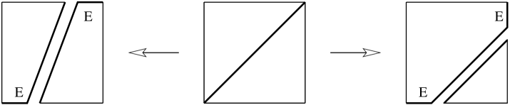
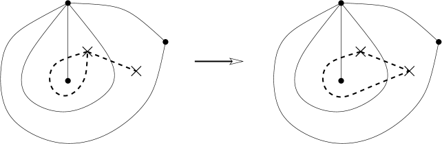
We remark that if the differential yielded a WKB triangulation which contained a self-folded triangle, the dual cellulation would contain an edge with goes from a zero to itself, and the matching sphere construction would yield an immersed Lagrangian sphere in . The quiver prescription of Labardini-Fragoso then involves replacing this immersed sphere with an embedded replacement, as in Figure 4. In any case, the situation covered by Lemma 2.2 will suffice in this paper.
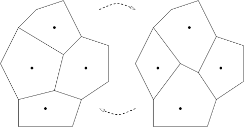
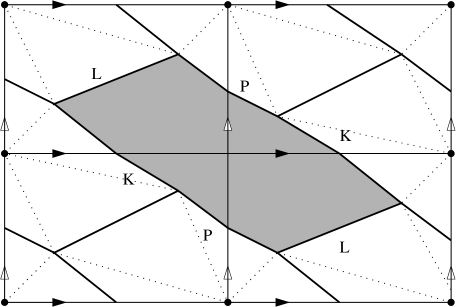
Saddle-free differentials form chambers which are separated by walls on which, in the simplest instance, there is a unique saddle connection; the corresponding triangulations differ by a flip, and the Lagrangian cellulations and WKB collections differ as in Figure 5, assuming the WKB triangulations are non-degenerate on both sides of the wall.
Note that the Lagrangians , for two distinct edges may meet at two points, cf. Figure 6. In this case, the union of the two matching paths is necessarily a homotopically non-trivial loop, by the uniqueness of geodesic representatives for homotopy classes in complete flat surfaces, see [54].
Remark 3.22.
A holomorphic quadratic differential on has zeroes. There is no trivalent cellulation of with vertices the zeroes of , for reasons of Euler characteristic (trivalence implies the number of faces would be zero). Thus, there is no direct analogue of the Lagrangian cellulation for the 3-fold of Equation (3.1).
3.10. Gradings
Let be a symplectic manifold with , so that has trivial bicanonical bundle , where is defined with respect to any compatible almost complex structure. The space of possible homotopy classes of trivialisation of is given by . Pick a quadratic volume form giving the trivialisation. defines a map from the Lagrangian Grassmannian to the circle
For any there is an induced map and a grading of is given by a phase function with . If , are graded Lagrangians, any isolated transverse intersection point of and acquires an absolute Maslov index .
Example 3.23.
Suppose is the graph of an exact one-form in , and is Morse with an isolated critical point at . Equip with the constant trivial phase function. There is a distinguished choice of grading on compatible with the canonical isotopy from to via graphs of , and with respect to this grading, is given by the Morse index of as a critical point of .
The Lagrangian submanifolds admit gradings with respect to the holomorphic volume form of Lemma 3.6, since they are simply-connected.
Since equips the surface with a flat metric with singularities, a curve has a well-defined phase at each point with . Recall that is a geodesic for the -metric precisely if this phase is constant on each connected component of , and any primitive saddle connection for is a geodesic.
Lemma 3.24.
There is a volume form homotopic to with the property that the phase function of the matching sphere , computed with respect to , is equal to the -phase of the curve . In particular, saddle connections define Lagrangian 3-spheres of constant phase.
Proof.
Away from a neighbourhood we have a holomorphic -action on fixing the divisor at infinity, hence the associated holomorphic volume form is -invariant in this subset. It follows that the phase function on a matching sphere is -invariant, where rotates the -fibres, hence defines a function on the underlying matching path . We claim that this function co-incides with the phase of in the -metric.
The result is local, so after passing to a cover of we can reduce to the case where is an arc in the base of a Lefschetz fibration with fibres given by affine quadrics. An explicit formula for the phase can then be obtained from the Poincaré residue theorem, compare to [56, Section 6] or [29, Section 5e]. In particular, for the local model
equation (6.3) of [56] asserts that the phase function associated to at any tangent vector to the Lefschetz thimble defined by a path , and projecting to , has phase , i.e. that pushes forward to the one-form . Thus defines a quadratic differential on the -plane with a simple zero. ∎
The previous Lemma can be used to fix the phase of uniquely.
4. Floer theory
4.1. Almost complex structures
The manifold is not convex or of contact type at infinity, because the divisor is not ample. Lemma 3.10 nonetheless gives good control on holomorphic curve theory in .
Definition 4.1.
Let denote the space of almost complex structures on which
-
(1)
tame the symplectic form ;
-
(2)
make projection holomorphic;
-
(3)
co-incide outside a compact set with the restriction of the integrable complex structure from the crepant resolution .
Lemma 4.2.
For there is no non-constant -holomorphic map , and if is a matching sphere, then bounds no -holomorphic disk.
Proof.
Since projection is holomorphic and , the first statement follows. The same argument implies that any -holomorphic disk with boundary on is contained in a fibre of the projection , but the intersection of with any fibre it meets is exact. ∎
A pseudoholomorphic disk denotes the solution to a perturbed Cauchy-Riemann equation
| (4.1) |
defined on a disk with boundary punctures and Lagrangian boundary conditions , where is a 1-form and the Hamiltonian vector field of a Hamiltonian function which vanishes to order at least 2 on the divisor . The -part of the 1-form is taken with respect to a family of almost complex structures induced by a mapping of the domain of into . Note that the map has the property that is some fixed integrable structure near . In local co-ordinates Equation 4.1 has the form
Since near and is constant near infinity, outside a relatively compact subset whose interior contains all the , Equation 4.1 reduces to the usual unperturbed holomorphic curve equation.
Lemma 4.3.
Let be compact Lagrangian submanifolds, and suppose is a sequence of pseudoholomorphic disks with uniformly bounded energy and with boundary on . Then the are contained in some compact subset of .
Proof.
Suppose the conclusion of the Lemma fails. By Gromov compactness in the smooth variety , some subsequence of the converges to a curve in which has non-trivial intersection with the divisor . Since the Cauchy-Riemann equation is unperturbed near infinity, the image of must meet locally positively, except for components contained inside the divisor. More precisely, positivity of intersections applied to the principal component of the stable curve limit means that this limit curve must contain at least one bubble component which is a rational curve in with strictly negative intersection with . No such curves exist by Lemma 3.10. ∎
4.2. Fukaya category generalities
The strictly unobstructed Fukaya categories occuring in this paper belong to a technically manageable regime. The relevant transversality theory is encompassed by material in [47, 49], to which we defer for essentially all details of the construction.
Let be a symplectic manifold which admits a class of taming almost complex structures which satisfy the first conclusion of Lemma 4.2. We only consider strictly unobstructed Lagrangian submanifolds, and suppose furthermore that the conclusion of Lemma 4.3 is valid. (A quasi-projective variety admitting a compactification as in Lemma 3.10 is the most relevant source of examples.) For ach there is a -graded -category , linear over , called the strictly unobstructed (-twisted) Fukaya category. Objects of are Lagrangian branes , namely:
-
•
is a closed oriented Lagrangian submanifold;
-
•
is an almost complex structure for which bounds no -holomorphic disk and meets no -holomorphic sphere;
-
•
carries a relative spin structure, relative to the class ;
-
•
is graded, see Section 3.10.
Morphisms in are given by the Floer cochain complex , which is freely generated by intersection points of and if they intersect transversely. More properly, index theory and the choice of gradings on , associate to any isolated transverse intersection point an abstract one-dimensional -vector space , see [47, Section 11h], and the Floer complex
There are higher order chain-level operations which comprise a collection of maps
| (4.2) |
of degree , for , with being the aforementioned differential and the holomorphic triangle product. The have matrix coefficients which are defined by counting holomorphic disks with -boundary punctures, whose arcs map to the Lagrangian submanifolds in cyclic order and which converge in strip-like end co-ordinates at the punctures to intersection points. The moduli spaces of disks are naturally oriented relative to the orientation lines occuring in (4.2) (in a manner which depends on the choice of ), so the count of pseudo-holomorphic disks is a signed count. The count of a disk is weighted by the symplectic area , with the Novikov parameter.
The construction of the operations is rather involved, and we defer to [49, Section 3] for details; in particular, the coefficients depend on additional perturbation data (choices of Hamiltonian functions, domain-dependent almost complex structures, strip-like ends etc; these choices in part overcome the difficulty that a Lagrangian is never transverse to itself). The coefficients are not individually well-defined (the are not chain maps), but the entire structure is invariant up to a suitable notion of quasi-isomorphism. Hamiltonian isotopic Lagrangian submanifolds, equipped with brane data compatible with the isotopy, define quasi-isomorphic objects of .
We denote by the category of twisted complexes over , and by its idempotent completion. The corresponding cohomological categories are denoted and .
We record one particular fact for later.
Lemma 4.4.
Let be supported by a locally finite cycle disjoint from a collection of spin Lagrangian submanifolds . Suppose the are pairwise transverse, and fix intersection points with cyclic indices. If a rigid holomorphic disk contributes to the coefficient with value , then it contributes to the same coefficient in with coefficient , where is the algebraic intersection number of the disk with the cycle .
Proof.
See [14, Vol. II, Proposition 8.1.16]. Since , each of the spin Lagrangians is also relatively spin relative to . Note that two Hamiltonian isotopic representatives for in each lying in , which define quasi-isomorphic objects of , may not be Hamiltonian isotopic in . The trace on of the isotopy with the cycle defines a -cycle in , Poincaré dual to a class in which twists its relative spin structure compatibly with the change in intersection number with of some given element in . ∎
If one encounters Lagrangians in some convenient geometric position (clean Morse-Bott intersections, matching cycles in a Lefschetz fibration) it is often useful to compute without perturbing them. Given a finite set of Lagrangians which meet pairwise transversely, one can define the corresponding Fukaya category subject to this constraint, but the stucture coefficients are obtained from (virtual) counts of more general objects called pearly trees, see [48, Section 7] and [51, Section 4].
First, one defines for a fixed Morse function (Morse-Smale for an underlying Riemannian metric). An abstract pearly tree is a planar tree with one infinite incoming and several infinite outgoing edges, and finite-length internal edges, vertices of valence at least 3, the connected components of the complement being labelled by Lagrangians . A holomorphic pearly tree comprises a collection of pseudoholomorphic disks and gradient flow-lines, satisfying obvious incidence and compatibility conditions; gradient flowlines arise when computing a higher product for which some inputs , see Figure 7.
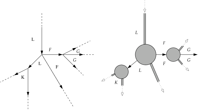
There are two important situations in which one can avoid pearls for purposes of computing a coefficient of (4.2).
-
(1)
If adjacent boundary conditions (with cyclic indices) are always pairwise transverse, in particular never co-incide, there are no pearly contributions to this particular coefficient of . This relies on an important theorem due to Sheridan [51, Proposition 4.6]: moduli spaces of pearls can be made regular by generic choices of consistent perturbation data, and in the regular case pearls with internal edges form a stratum of real codimension . Therefore for isolated regular pearls, there are no internal (finite length Morse) edges of the underlying planar tree.
-
(2)
If there is exactly one adjacent pair of co-incident Lagrangians , and the corresponding input or output is the class of top degree, then one can count pseudoholomorphic polygons which are smooth at the given corner but have an incidence condition, passing through a fixed generic point Poincaré dual to . Compare to [48, Section 7].
The choice of as background class is relevant in Lemma 4.11, but much of the discussion in the next sections applies to the categories uniformly. We will sometimes omit the background class from our notation when it plays no role.
4.3. Grading the WKB algebra
Now return to the 3-fold . Any Lagrangian matching sphere is strictly unobstructed and admits a unique spin structure. Since bounds no holomorphic disks, the cohomology , equipped with its classical -structure.
Given a finite collection of Lagrangian spheres , and a choice of , there is an associated total morphism -algebra
| (4.3) |
Theorem 1.1 involves computing the -algebra , where the indices are indexed by edges of a non-degenerate triangulation and correspond to a WKB-collection of Lagrangian spheres, and identifying it with the corresponding Ginzburg potential algebra (i.e. with the total endomorphism algebra of the category considered in Section 2.1).
Lemma 3.19 implies that each can be taken to fibre over the path , and hence it suffices to compute the Floer theory amongst such a collection of fibred matching spheres. By projecting to , pseudoholomorphic disks are then constrained by the Riemann mapping theorem. Collections of matching spheres don’t lie in general position (there are triple intersections at vertices of the Lagrangian cellulation), so in principle one must define via pearls, but the remarks at the end of Section 4.2 imply that in the case at hand the consequences are fairly benign.
Consider the Lagrangian submanifolds which are matching spheres for the edges of the Lagrangian cellulation (dual to a non-degenerate WKB triangulation). Any two distinct Lagrangians are either disjoint or meet at either one or two isolated points, lying over trivalent vertices of the cellulation (the nodal points of a fibre of lying over a zero of ).
Lemma 4.5.
The admit gradings for which
-
•
the algebra is concentrated in degrees ;
-
•
the isolated intersection points have absolute Maslov index clockwise and anticlockwise, cf. Figure 8.
Proof.
The groups carry their natural grading, and by Poincaré duality for any , so it suffices to determine the grading of an isolated intersection point lying over a zero of . The Lagrangian matching paths of a WKB-type Lagrangian cellulation are realised by geodesics for the -metric on , so the Lagrangians are locally given by transversely intersecting special Lagrangian thimbles.
More explicitly, working locally near a simple zero of the quadratic differential , we consider the three straight arcs of the associated vertical foliation, which form the terminals of a trivalent vertex. (Comparing to Figure 5, the leaves of the horizontal foliation at a zero fall into the double poles at the centres of the three cells adjacent to the zero, and the edges of the Lagrangian cellulation are given, locally near the zero, by leaves of the vertical foliation.) Each of the arcs defines by parallel transport a Lagrangian disk in the 3-fold , and Lemma 3.24 implies these all have identical phase. There are Darboux co-ordinates in which these three Lagrangians are given by linear subspaces and . (Note the quadratic volume form is invariant under rotation by , just as the quadratic volume form on , locally given by with , is locally invariant under rotation by .)
is the graph of the differential of a function over with an isolated minimum, so a Morse critical point of index . Therefore, for the grading on compatible with the obvious rotation isotopy back to , the absolute index would be zero by Example 3.23. The phase function differs from the phase function compatible with that isotopy by the constant function , hence the index of the intersection point is . (An alternative for the last step is to use non-vanishing of the triangle product, Lemma 4.9 below, to show that since the absolute indices are symmetric under rotation of Figure 8 by , they must all equal .) ∎
The local Morse-theoretic description of an isolated intersection of WKB spheres given above also yields preferred isomorphisms between the orientation lines and the ground field, coming from preferred trivialisations for the determinant line of a -operator on a half-plane with linear Lagrangian boundary conditions which rotate by . Via these trivialisations, Lemma 4.5 shows that the WKB algebra is isomorphic, as a graded vector space, to the total morphism algebra of the category introduced in Section 2.1.
4.4. First constraints on polygons
Let be matching spheres which are edges of a non-degenerate WKB cellulation. Appealing to [47, Lemma 2.1], we can take the -structure on the algebra from (4.3) to be strictly unital.
Lemma 4.6.
Let . If the product
is non-zero, then either and all inputs have degree , or , exactly one input has degree and all others have degree .
Proof.
Lemma 4.5 implies that the degree subalgebra of the WKB algebra is spanned by the units of the constituent WKB spheres. It follows that since the -structure is strictly unital, none of the inputs to a non-trivial operation with has degree . Hence every input has degree , whilst has degree . Since is concentrated in degrees , it follows that no input can have degree , and at most one input can have degree . Moreover, there is an input of degree if and only if the output has degree , which is possible only if and co-incide. ∎
Lemma 4.7.
The second case of Lemma 4.6 does not occur.
Proof.
Working with pearls, we take a Morse model for self Floer cochains; without loss of generality, for each WKB sphere we can take a perfect Morse function so the Floer cochain group has rank 2. If there is a degree two input to the product in Lemma 4.6, the output is in the rank one space , which means that the holomorphic disk should pass through the stable manifold for the gradient flow of the maximum of the Morse function on . Therefore this marked point is unconstrained, and hence no non-constant disk can be rigid. It follows from the proof of Lemma 4.9 below that constant polygons contribute non-trivially to but not to for . ∎
According to [13, Theorem 1.1], over the Fukaya category can always be taken both cyclic and strictly unital, and Lemma 4.7 would also follow formally from that fact, compare to Section 2.1. A helpful consequence of the previous result is that one can compute the Fukaya category using pseudoholomorphic disks rather than pearly trees. Note that these results do not imply that all the in (4.2) are pairwise distinct for the corresponding operation to be non-trivial, see Figure 9 for an example.
The boundary of any holomorphic polygon contributing to defines a (not necessarily embedded) parametrized closed path in the graph on the surface formed by the edges of the Lagrangian cellulation. Inputs of degree correspond to turning clockwise in the graph defined by the cellulation edges, and inputs of degree correspond to turning anticlockwise, along the boundary of the disk; it is simplest to see this by lifting the disk to the universal cover, given by pulling back the fibration to the universal cover of , where the Lagrangian cellulation edges give rise to a trivalent planar graph. Lemma 4.6 implies that there is at most one anticlockwise turn.
Example 4.8.
Suppose and meet transversely at a single point. The unique closed path of length gives rise to the product
| (4.4) |
which is non-trivial by Poincaré duality.
4.5. Constant triangles
Let be three graded Lagrangian submanifolds, intersecting pairwise transversely at a point . There is a constant holomorphic triangle with boundary conditions (anticlockwise ordered) . Let be the linearized operator at , i.e. the -operator on the trivial vector bundle with fibre over a disk with three boundary punctures, with boundary values in , , . The index formula for such operators [47, Proposition 11.13] implies that
| (4.5) |
We now return to the situation (and notation) arising in the proof of Lemma 4.5. We label the linear Lagrangians and by , and , corresponding to the slopes in the complex plane of the arcs over which they fibre in the model Lefschetz fibration
For the zero phase functions of Lemma 4.5, the indices appearing in (4.5) are
so the constant triangle has index and can in principle contribute non-trivially to the product in the algebra .
Lemma 4.9.
The constant holomorphic triangle at a trivalent zero contributes exactly to a non-trivial multiplication
Proof.
The local model splits into a direct sum of 3 copies of the geometry given by 3 real lines in passing through the origin.
The regularity of the constant triangle is then standard, provided the Lagrangians are taken in the appropriate order. For a constant triangle in contributing to a product
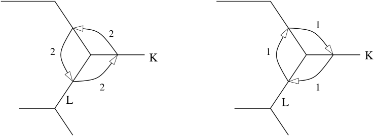
the indices are as given in Figure 10 (consider perturbing the three lines to create a non-trivial triangle in , which is either holomorphic or antiholomorphic depending on the cyclic order of the boundary conditions). ∎
Constant triangles and Poincaré duality do not always completely determine the algebra structure in ; there may be additional products if some of the cells of the Lagrangian cellulation are themselves triangles.
4.6. Holomorphic disks on totally real cylinders
Constant holomorphic triangles provide the cubic terms in the superpotential associated to a triangulated surface arising from the “inscribed triangles” of Labardini-Fragoso’s quiver prescription for a potential [32], see (2.2) and Figure 1. The higher order terms of the potential arise from higher order -products in . En route to computing these, it will be helpful to study a simpler local model involving the Lagrangian cylinder of Section 3.8.
Recall the totally real model for the Lagrangian cylinder given in (3.13). We will consider holomorphic sections with this boundary condition.
Lemma 4.10.
In the notation of Lemma 3.21, there are exactly two rigid holomorphic sections of with boundary condition on , and all other moduli spaces of sections are empty.
Proof.
Consider a section of . Since , each co-ordinate projection defines a holomorphic map . In the co-ordinate this is a map from the unit disk to which takes the boundary circle to the real line; any such is constant, so in fact the non-trivial geometry takes place in the -bundle over the disk with co-ordinates . In each of these factors, the total space of the fibrewise Lagrangian of Equation 3.13 over the boundary circle defines a Möbius band, for instance
Consider a holomorphic section of in this factor. This defines a map on the disk with the property that for . [45, Lemma 2.16] shows that the only holomorphic maps satisfying on are
Therefore if is a holomorphic section of , then , but then is meromorphic with a pole, unless . It follows that the only holomorphic sections of with boundary condition are the constant sections
Since the sections are constant, they are both regular. ∎
We equip with the unique spin structure which is bounding in the circle factor. The moduli space of holomorphic sections of with boundary on inherits a canonical orientation. (More precisely, we are interested in the space of sections with a single boundary marked point, which has a natural evaluation map to .) Note that this spin structure is in particular a relative spin structure relative to the class of (1.3), since . The choice of background class enters the computation of at the following point.
Lemma 4.11.
The two rigid sections of Lemma 4.10 contribute to the moduli space of sections with opposite signs, with respect to the trivial background class , and with the same sign, relative to the background class .
Proof.
We return to the local model of Lemma 3.21, and the affine variety . There is a holomorphic involution of the model given by , . This acts fibrewise, preserves the Lagrangian , and exchanges the two holomorphic sections. The involution preserves the orientation of , which implies that the sections count with the same respectively opposite signs (for the trivial background class) depending on whether or not the involution does or does not preserve the stable trivialisation of the Lagrangian boundary condition along the sections determined by the spin structure on , cf. [14, Proof of Theorem 8.1.1]. We claim that the involution does not preserve this stable framing.
Fix a model , with the bounding spin structure. Let denote co-ordinates on the -factor. There is a natural parametrisation taking to
The involution acts fibrewise on the -factor of by reversing the sign of and reflecting the circle in the -plane along an axis of angle . Altogether, this means we act by the generator of and hence of . Put differently, the boundary values of the holomorphic sections, viewed as -submanifolds of , have an obvious “constant” framing (constant in a twisted parametrisation) from the tangent spaces to the -plane. These “constant” framings are exchanged by the involution, but are not simultaneously compatible with a choice of spin structure on . Indeed, is really the mapping torus of a rotation by on , and the two holomorphic sections have boundary values coming from the two rotation fixed points. Homotoping the monodromy to the identity rotates the tangent spaces at the fixed points by in opposite directions, hence can bring only one of the two “constant” framings to the framing induced by the fixed spin structure. The upshot is that the two sections contribute with opposite signs to the moduli space oriented with respect to the trivial background class.
Note that is supported by a locally finite cycle disjoint from the Lagrangian . The two holomorphic sections of Lemma 4.10 each hit one of the two components of the reducible fibre over the local point of , hence exactly one of them intersects , so turning on the background class changes the sign of exactly one of the disks by Lemma 4.4. ∎
Remark 4.12.
After twisting by , the boundary values of the sections of Lemma 4.10 sweep the 1-cycle
which is not the restriction of any central element of . Therefore a Lagrangian cylinder has obstructed -twisted Floer cohomology, and does not define an object of , even if one enlarges the category to allow unobstructed branes in the sense of [14] rather than just weakly exact Lagrangian submanifolds.
4.7. Nonconstant polygons
Fix a finite collection of matching spheres arranged cyclically, bounding an open subset of containing a unique double pole of . The Lagrangians meet at a sequence of intersection points for (with by definition). Appealing to Lemma 4.5, we may suppose that has Maslov index . Let denote the dual Maslov index 2 intersection point which is a generator of .
Lemma 4.13.
If the are pairwise distinct, the coefficient of in the product
is well-defined; it is independent of the auxiliary choices made in constructing the Fukaya category.
Proof.
Recall that the construction of the Fukaya category relies on additional perturbation data of Hamiltonian deformations, domain-dependent almost complex structures or Morse-Smale pairs made universally over moduli spaces of stable disks or pearly trees. As in [47, Section 10e], two different choices of that auxiliary data , , for defining the -operations can be related by a continuation -functor between the resulting Fukaya categories . Given a configuration of WKB Lagrangians, (the action on morphism groups) is necessarily the identity, whilst also vanishes on (defining self-Floer cochains using perfect Morse functions). The -functor equations then imply that
| (4.6) | ||||
The higher products amongst the all vanish for , since any contributing holomorphic disk would not have boundary defining a closed curve in the WKB-graph. That immediately implies the -product is invariant under . ∎
Note that the hypothesis that the are pairwise distinct can be weakened to the hypothesis that no cyclic subchain arises as the ordered boundary of any non-trivial element of . Since holomorphic disks lift uniquely to unramified covers, it would also be sufficient to realise either of these hypotheses after pullback to a covering space, as in Figure 9.
Suppose one has a Lefschetz fibration and a finite collection of cyclically ordered weakly exact matching spheres which enclose a disk containing no critical points of . Suppose that the Lagrangians are pairwise distinct, and have the obvious affine -intersection graph. Let denote the intersection points, for with cyclic indices. The following is well-known, and reflects the existence of a relation between the classes .
Lemma 4.14.
If denotes the unit,
| (4.7) |
Proof.
Remark 4.15.
Suppose is a holomorphic quadratic differential, and consider a cycle of matching spheres in the 3-fold of (3.1) enclosing a disk with no critical points of , hence in the configuration of the previous Lemma. The non-vanishing of this higher product implies that , which precludes for every . It follows that is not described by a quiver with potential of WKB-type. Compare to Remark 3.22.
The higher product of (4.7) counts disks with punctures, which extend smoothly across the output puncture but are constrained at the corresponding marked point on the boundary of the disk to pass through a generic point , the minimum of the Morse function used to define . In particular, consider the moduli space of Maslov zero holomorphic polygons with punctures at the given intersection points, and one boundary marked point on the boundary interval between the first and last inputs. The -relations then imply that for generic , is a closed manifold of dimension . There is an evaluation map
| (4.8) |
which is transverse for generic choices of perturbation data, and Lemma 4.14 implies that
| (4.9) |
Lemma 4.16.
For background class , the contribution to the multiplication
from holomorphic disks which project to a single WKB cell with multiplicity one is non-trivial.
Proof.
We are essentially in the situation of Lemma 4.13, bearing in mind the remark after that Lemma. Note that our standing hypotheses imply that , so the number of faces of the Lagrangian cellulation associated to a non-degenerate WKB triangulation is at least 2. In particular, given any face of the cellulation, there is at least one boundary edge on that face which occurs exactly once in the boundary, separating two distinct embedded open faces on the surface . (This need not be true when , see Figure 9.)
Following a well-known strategy going back at least to [45], we then apply a degeneration and gluing argument to the situation depicted on the left of Figure 11, which is a schematic for a polygon of matching spheres encircling a double pole in .

There is a Lagrangian boundary condition fibred over the dashed circle, and Lemma 4.11 asserts that the algebraic count of isolated holomorphic sections over this inner disk is non-vanishing. There is a degeneration of the restriction of the fibration to this WKB cell, indicated on the right of Figure 11, to a pair of fibrations over disks with boundary marked points, namely the local model and the trivial fibration over a polygon encircling no singular fibres. In this degeneration, we push the double pole towards an edge which occurs only once on the boundary on the given polygon, so the degeneration on the surface is locally schematically well depicted by Figure 11. The gluing theorem [45, Proposition 2.14] implies that
| (4.10) |
where denotes the -dimensional component of a space of holomorphic sections over the relevant domain, is the boundary marked point on the fibrations after degeneration, and the fibre product is taken over evaluation into the Lagrangian 2-sphere . The evaluation maps are transverse for generic , see e.g. [36, Proposition 3.4.2]. On the right of Equation 4.10, we have computed already that is trivial except for ; on the other hand, Lemma 4.14 and (4.9) imply that the evaluation map sweeps with multiplicity 1. The fibre-product is therefore non-empty; the moduli space on the left of Equation 4.10 is cobordant to two (transversely cut out) isolated points.
Since the two holomorphic sections contribute to with the same sign by Lemma 4.11, given our choice of background class , the holomorphic polygons contribute to with the same sign.∎
If the conic fibres of over points in had a different topological type (smooth, Lefschetz singularities, higher multiplicity, empty etc), or if we took , it seems the analogue of Lemma 4.16 would not hold.
4.8. Summary
Fix a non-degenerate triangulation of which satisfies the conditions of Theorem 2.1. Denote by the associated Ginzburg category from Section 2.1, for the trivial signing . Via Lemma 2.2, pick a meromorphic quadratic differential whose associated WKB triangulation is . Let denote the corresponding WKB Lagrangian spheres, graded as in Lemmas 4.9 and 4.16, and denote by the total morphism algebra in the category .
Theorem 4.17.
Suppose . The -algebra is quasi-isomorphic to .
Proof.
We begin by recalling the discussion from the end of Section 4.3. The -algebra is the total morphism algebra of an -category over whose objects are the Lagrangians , which correspond one-to-one with the vertices of the quiver . From Lemma 4.5 we know that each has Floer cohomology isomorphic as a graded algebra to , and the morphisms between the different are based by the arrows in the quiver , graded as in the construction of the category in Section 2.1. Thus, as graded vector spaces, are isomorphic.
Floer theory equips with an -structure which, by homological perturbation, we can take to be minimal and strictly unital. The structure coefficients of this -structure count holomorphic polygons with boundary conditions the , weighted by their symplectic areas. Lemmas 4.6 and 4.7, together with Poincaré duality as in Example 4.8, imply that in the notation of Equation 2.1 the only non-trivial multiplications in with are exactly those recorded by the corresponding cyclic degree maps , i.e. the -structure is in fact cyclic. It follows that the -structure on may be encoded by the terms of a reduced potential on .
Lemma 4.9 implies that there is a non-trivial multiplication in , and hence non-trivial cubic term in the potential , for each isolated intersection point of a triple of Lagrangians ; indeed, the corresponding Floer product counts a constant disc (of area zero) with co-efficient . Such isolated triple intersections exactly correspond to the clockwise 3-cycles for the faces of the triangulation , and show that the potential , where by definition is disjoint from . More prosaically, disjointness asserts that none of the oriented 3-cycles corresponding to the oriented triangular faces of centred on vertices of occur in (each triangular face of defines three such 3-cycles, pairwise cyclically equivalent).
Lemma 4.16 implies that there are further non-trivial multiplications in for each -dimensional face of the WKB Lagrangian cellulation on defined by . The corresponding coefficients in the potential are exactly the (anticlockwise-oriented) cycles occuring in the quiver (cf. Figure 1). In the notation of Lemma 4.13, Lemma 4.16 implies that the Floer product is a non-zero multiple of , where the multiple depends on the symplectic area of the polygons occuring in Lemma 4.16 and the orientation (relative to the orientation lines associated to intersection points) of that moduli space: we have established (via Lemma 4.11) that the two holomorphic sections which contribute to the given product count with the same sign, hence cannot cancel, but have not pinned down that sign. At this stage, we may therefore write the potential as
| (4.11) |
where we sum over the faces respectively vertices of , where records the area and orientation of the holomorphic discs of Lemma 4.16, and where is disjoint from the various cycles and . Since (with the isomorphism arising from the Leray-Serre spectral sequence of the projection map), the choice of symplectic form not only determines but is essentially equivalent to a choice of (non-zero) scalar coefficients above.
At this point, we have determined the -structure constants which arise either from constant holomorphic polygons or from polygons which project to a single face of the WKB cellulation of with multiplicity one. In general there will be additional polygons, for instance those which project to a single cell with higher multiplicity (corresponding to powers of the cycles ) or to the union of two adjacent cells (corresponding to a concatenation ), which give rise to the terms in . Rather than determining these by hand, we appeal to finite determinacy, via the work of Geiss, Labardini-Fragoso and Schröer. Equation 4.11 shows that the potential governing the -structure on is exactly of the form given in Equation 2.3. By Theorem 2.1, we infer that the potential is weakly right-equivalent to , which shows that are -quasi-isomorphic as required. ∎
We should point out that analogous finite determinacy arguments have been used to pin down -structures in symplectic topology elsewhere, going back at least to Seidel’s [48].
Since the quiver category is independent, up to derived equivalence, on the particular WKB triangulation , one can infer the same result for the subcategories of generated by the Lagrangians coming from different cellulations (strictly, provided those cellulations come from triangulations satisfying the hypotheses of Theorem 2.1). Since is idempotent complete, Theorem 4.17 then implies that
Since is tautologically a subcategory of the Fukaya category , on passing to twisted complexes and then cohomology we see that , which completes the proof of (the first case of) Theorem 1.1 as stated in the Introduction.
4.9. Generation
Fix a non-degenerate triangulation . This subsection outlines one approach to proving that generates the subcategory generated by all matching spheres. This sketch falls far short of a proof, but it seems worth including in part because one sees the Harder-Narasimhan filtration of a matching sphere with respect to the stability condition determined by emerge as a natural ingredient in the argument.
There are two pieces of background for the sketch. Let and denote two matching spheres which meet transversely once, at a vertex of the cellulation. Consider the Lagrange surgery of and at , which is equivalently given by taking the Dehn twist of about . (There are two local surgeries, corresponding to the positive and negative Dehn twists; here we are taking , a morphism from to .) Seidel’s theorem [45] yields a distinguished triangle in
| (4.12) |
This gives a long exact sequence of Floer cohomology groups in
for any third Lagrangian submanifold , and shows the Lagrange surgery is generated by the two constituent Lagrangians and .
The second piece of background concerns Floer theory for immersed Lagrangians [3]. Consider a closed saddle trajectory for of phase , going from a zero to itself. If we assume that the residue of at each double pole does not belong to , then forms one boundary component of a ring domain, the other boundary of which is a union of straight arcs also of phase (the hypothesis on the residues rules out the degenerate case in which the other boundary component collapses onto a double pole). The closed saddle defines an immersed Lagrangian 3-sphere . Despite being immersed, this has well-defined Floer cohomology (indeed is still strictly unobstructed, i.e. bounds no holomorphic disks, so this is straightforward), and
where the second summand arises from the node of .
The suggested route to generation of by has three ingredients.
Step 1. Let be as above, and suppose for simplicity that both boundaries of the ring domain containing are composed of a single saddle (this is true for generic , compare to the discussion of hat-proportional saddles in [5, Section 5]).

Let be two -geodesics inside the ring domain bound by , as in Figure 12, defining embedded matching spheres , in with
where denote the zeroes on the boundary of the ring domain and belongs to . It seems natural to conjecture that the immersed sphere is quasi-isomorphic to the cone
| (4.13) |
This is a version of (4.12), in a setting where the surgery is unobstructed but immersed (in particular cannot be interpreted in terms of a Dehn twist). One roundabout approach to a proof of (4.13) would appeal to known results on homological mirror symmetry for the 3-dimensional affine -singularity, which provides a local model for two spherical objects having a two-dimensional space of extensions, cf. the discussion of the representation theory of the quiver (J1) in [5, Section 11].
Step 2. The existence theorem for geodesics in flat surfaces implies that a given matching path is homotopic to a concatenation of -geodesics , where each is embedded in its interior (hence is either a geodesic matching path or a closed geodesic from a zero to itself). Given the correspondence between geodesics and stable objects [5, Theorem 1.4], this decomposition should reflect the Harder-Narasimham filtration of in the stability condition associated to , and (especially in light of [56]) there are obvious potential connections to mean curvature flow. In particular, one expects that , where denotes the extension-closed subcategory generated by the given objects. An inductive argument might reduce that claim to the special cases of the surgery exact triangle discussed above.
Step 3. At this point, one would know that any Lagrangian matching sphere is generated by the subset of matching spheres coming from -geodesics. An embedded -geodesic of phase occurs as one of the WKB-Lagrangians for the cellulation associated to , for sufficiently small , compare to [5, Figure 32]. If the triangulation associated to this rotated differential is non-degenerate, it is immediate from Theorem 1.1 and the fact that that is generated by the category associated to the triangulation defined by itself.
However, if has a triangulation with self-folded triangles, this is more delicate. To conclude that generates , at least by this method, one would need further to introduce the algebras for arbitrary, not necessarily non-degenerate triangulations , and to prove that in this wider setting. Note in particular that any such argument would seem to hinge on an extension of the results of [18] to this more general setting. Assuming that such an extension had been carried out, however, one could then conclude the desired generation: would be generated by geodesics, geodesics arise as WKB-Lagrangians for some triangulation, and all the subcategories of associated to triangulations would be quasi-equivalent.
5. Miscellany
5.1. Higher order poles
Suppose we have a marked bordered surface with , arising from a quadratic differential on a Riemann surface with a non-empty set of poles of order . We construct the 3-fold as indicated in the Introduction.
The preceding arguments need only minimal changes to yield the second case of Theorem 1.1. The locally free sheaf now has first Chern class , in the notation of (1.2). The proof of Lemma 3.5 then implies that the projective completion has canonical class , which again means that after removing the open 3-fold is a smooth Calabi-Yau222Since the coefficients in the divisor are all , the holomorphic volume form again has poles of order at least 2 at infinity.. It is moreover affine, and one can work with a symplectic structure which is exact and contact type at infinity, which obviates the need to control rational curves via intersection theory at infinity.
Lemma 3.14 changes. We now view the differential as a section of the bundle , where the divisor , which means has simple zeroes at odd order poles, and hence the local system picks up monodromy at odd order poles. The identification of with the anti-invariant homology of a spectral double cover goes through only if that cover is branched at both zeroes and odd order poles. The upshot is that is now free of rank
Lemma 3.11 carries over unchanged. The construction of symplectic forms, matching spheres, and the grading of the WKB algebra, were all essentially local arguments on , as were the computations of the contribution of constant holomorphic triangles and non-constant polygons covering WKB cells with multiplicity one. At this stage, one sees that the -structure on the WKB algebra is given by a potential of the shape as before. Finally, the crucial result Theorem 2.1 of Geiss, Labardini-Fragoso and Schröer also holds in the non-empty boundary case (with no further constraints on the number of punctures), which enables one to conclude the proof as before.
Example 5.1.
Consider to be an annulus with respectively marked points on the two boundary components. This corresponds to differentials on with poles of order and and simple zeroes. The quiver is a non-cyclic orientation of the affine -Dynkin diagram, with trivial potential. The Lagrangian spheres of a WKB collection form a cycle of matching spheres encircling the origin; the vanishing of the potential reflects the fact that the threefold fibres over , and there are no non-constant holomorphic polygons (by the maximum principle applied in ). Note that the poles of the holomorphic volume form and resulting grading of the endomorphism algebra of the WKB collection depend on the decomposition . Compare to [5, Section 12.3].
5.2. Simple poles
Whilst one can construct the triangulated category associated to by starting with a non-degenerate ideal triangulation defined by a point of the open stratum , the space of stability conditions on is (an orbifolded version of) the larger space in which the differentials may acquire simple poles by having zeroes collide with double poles. The universal family of threefolds (which exists locally) does not extend to as a locally trivial fibre bundle. In any extension of the universal family there must be a non-trivial degeneration of when acquires a simple pole, to account for the non-triviality of the monodromy action on described in Lemma 3.12, which exchanges components of the reducible fibre.
Return to the local model
for the neighbourhood of the reducible fibre inside , where has a double pole at and . Suppose instead that we have a differential with , so the quadratic differential has a simple pole at the corresponding point of . The corresponding 3-fold
has a multiple fibre , and is singular along a smooth conic curve . The transversal singularity is a surface ordinary double point.
It is tempting to associate to a quadratic differential with a simple pole at a smooth 3-fold
with fibre , with multiplicity 2, over . For suitable symplectic forms, there is a Lagrangian , fibred by a Morse-Bott function over an arc from a zero to (the vanishing cycle of the zero converges at to the Bott minimum). The two Lagrangian spheres depicted on the right side of Figure 4, which should persist in the category defined by since this does not change in passing from to , would now be realised by this , equipped with either the trivial or the non-trivial spin structure or equivalently -valued local system. It would be interesting to find a model (of this or another form) for the “locally trivial family of categories” over a point of the incomplete locus.
5.3. No poles
Let be a Riemann surface of genus . Consider again the 3-fold from (3.1) associated to a holomorphic quadratic differential on with distinct zeroes. This has a fibrewise compactification which is a Lefschetz fibration over with generic fibre . According to [53, Corollary 4.9], there is an equivalence of -graded split-closed categories
| (5.1) |
between the nilpotent summand of the Fukaya category of the even-dimensional quadric, i.e. that corresponding to the zero eigenvalue of quantum product with the first Chern class, and the Fukaya category of a pair of points (both categories are semisimple). The paper [53] works over , but the argument underlying the equivalence of (5.1) (which uses the computation of a certain Gromov-Witten invariant counting sections of a Lefschetz fibration with fibre and some elementary deformation theory) goes through over any algebraically closed characteristic zero field. Starting from this, one can show in the spirit of [53, Section 5] that, over the Novikov field , the -graded category underlying admits a formal deformation which is split-closed derived equivalent to the -graded Fukaya category of the spectral cover , i.e. the double cover of branched at the zeroes of .
That equivalence takes the matching sphere considered in this paper to the obvious circle lying over in the double covering . An essential simple closed curve defines a Lagrangian and a disjoint union of two circles in . The ring structures on the Floer cohomologies of these objects is different (only one has a non-trivial degree zero idempotent), which suggests that the deformation of categories from to induced by the compactification of the fibres is non-trivial.
5.4. The untwisted category
For each there is a total morphism algebra associated to a collection of Lagrangian matching spheres indexed by edges of a non-degenerate triangulation . The quasi-isomorphism type of this algebra will depend on the choice of , even though its idempotent pieces do not. Theorem 1.1 concerns the case and the twisted Fukaya category , and it is natural to consider the untwisted category corresponding to taking .
Lemma 4.11 determined the signs with which the two rigid disks with boundary on contribute to their moduli space. These discs cancelled in the category . Therefore, the category is obtained by replacing the potential of (2.2) by its first term , killing the higher -products; alternatively, it arises if one constructs the threefold by removing the conic fibres over all poles of , and not just those of order . This category is drastically different to , see the example considered in Section 5.5.
Moreover, in contrast to Remark 4.12, the Lagrangian cylinder does define an object of the untwisted category if one allows unobstructed branes. The category cannot be generated by matching spheres: the Lagrangian cylinder can be deformed through non-Hamiltonian deformations (shrinking the loop ) to be disjoint from any given matching path in , but (in the untwisted category) still with non-trivial Floer cohomology.
5.5. An example
Consider a differential on with poles of order and ; this case was considered in [5, Section 12]. The relevant quiver has two vertices and no arrows, and the category is generated by two Lagrangian spheres with . All objects are isomorphic to direct sums of shifts of the . These objects are depicted on the left of Figure 13, where the black dot denotes the double pole and the higher order pole lies at .

The vanishing of Floer cohomology relies on the choice of the non-trivial background class, which ensures the two rigid disks which project onto the obvious region bound by these arcs count with the same sign: the differential
| (5.2) |
maps the degree one generator to a non-trivial multiple of the degree two generator.
On the other hand, there are infinitely many pairwise non-Hamiltonian isotopic Lagrangian spheres in , distinguished in the split-closed twisted Fukaya category by the rank of Floer cohomology with the non-compact Lefschetz thimble dotted in the right of Figure 13 (with background class the differential in (5.2) vanishes, and spherical objects can then arise from non-trivial twisted complexes based on the ). Turning on the background class collapses all of these distinct objects onto shifts of and (direct sums are excluded by considering the rank of self Floer cohomology). Therefore isomorphism in the category is very far from implying Hamiltonian isotopy.
5.6. Open directions
It is natural to wonder if [5] and Theorem 1.1 have applications to the classical symplectic topology of , or to representation theory. The results established so far fall slightly short of what seems to be required, although there are several obvious avenues for further study.
There are natural representations (the first defined by parallel transport)
| (5.3) |
where the middle term refers to mapping classes preserving and where on the right we quotient by the square of the shift functor. It follows from results of [5] that if the space of stability conditions studied there is simply-connected, then the first arrow is injective: but simple-connectivity of is currently unknown (see however [40] for progress in this direction).
When one can kill the fundamental group of by subcritical handle attachments at infinity, to obtain symplectic six-manifolds which are simply-connected but admit symplectomorphisms of positive Floer-theoretic entropy, and which have subgroups of autoequivalences of the Fukaya category which surject onto mapping class groups. This may be of some interest, since whilst such examples are known, they are not yet terribly numerous.
In another direction, the second map of (5.3) does surject onto the quotient of the subgroup of autoequivalences which preserve by those which act trivially (“negligible” autoequivalences in the terminology of [5]). There are many situations in which autoequivalences of derived Fukaya categories have no geometric origin, i.e. do not arise from symplectomorphisms, see e.g. [2].
Finally, the existence of a smooth compactification divisor for gives rise to a spectral sequence computing symplectic cohomology , see [46]. That in turn leads to conjectural bounds on the ranks of the Hochschild cohomology groups of the Ginzburg algebra which might be of independent interest. It would be instructive, in this vein, to relate the wrapped Fukaya category of to the derived category of all (not necessarily finite-dimensional) modules over the complete Ginzburg algebra.
References
- [1] M. Abouzaid. On the Fukaya categories of higher genus surfaces. Adv. Math. 217:1192–1235, (2008).
- [2] M. Abouzaid and I. Smith. Exact Lagrangians in plumbings. Geom. Funct. Anal. 22:785–831, (2012).
- [3] M. Akaho. Intersection theory for Lagrangian immersions. Math. Res. Lett. 12:543–550, (2005).
- [4] D. Auroux, V. Munoz and F. Presas. Lagrangian submanifolds and Lefschetz pencils. J. Sympl. Geom. 3:171-219, (2005).
- [5] T. Bridgeland and I. Smith. Quadratic differentials as stability conditions. Preprint, available at arXiv:1302.7030.
- [6] C.-H. Cho and S. Lee. Potentials of homotopy cyclic -algebras. Homol. Homot. Appl. 14:203-220, (2012).
- [7] H. Clemens. Double Solids Adv. Math. 47:107-230, (1983).
- [8] D.-E. Diaconescu, R. Dijkgraaf, R. Donagi, C. Hofman and T. Pantev. Geometric transitions and integrable systems. Nuclear Phys. B. 752: 329-390, (2006).
- [9] A. Fathi, F. Laudenbach and V. Poenaru. Travaux de Thurston sur les surfaces. Asterisque 66-67. Soc. Math. de France, (1991).
- [10] A. Floer. Morse theory for Lagrangian intersections. J. Diff. Geom. 28:513-547, (1988).
- [11] S. Fomin, M. Shapiro, D. Thurston. Cluster algebras and triangulated surfaces, I. Acta Math. 201:83-146, (2008).
- [12] R. Friedman. Algebraic surfaces and holomorphic vector bundles. Springer, 1998.
- [13] K. Fukaya. Cyclic symmetry and adic convergence in Lagrangian Floer theory. Kyoto J. Math. 50:521–590, (2010).
- [14] K. Fukaya, Y.-G. Oh, K. Ohta and K. Ono. Lagrangian intersection Floer theory – Anomaly and obstruction, I & II. AMS Studies in Advanced Mathematics Vol. 46, International Press, (2009).
- [15] K. Fukaya, Y.-G. Oh, K. Ohta and K. Ono. Lagrangian Floer theory on compact toric manifolds, I. Duke Math. J. 151:23 174, (2010).
- [16] D. Gaiotto, G. Moore and A. Neitzke. Wall-crossing, Hitchin systems and the WKB approximation. Adv. Math. 234:239–403, (2013).
- [17] D. Galakhov, P. Longhi, T. Mainiero, G. Moore and A. Neitzke. Wild wall crossing and BPS giants. Preprint, arXiv:1305.5454.
- [18] C. Geiss, D. Labardini-Fragoso and J. Schröer. The representation type of Jacobian algebras. Preprint, arXiv:1308.0478, Version 2.
- [19] V. Ginzburg. Calabi-Yau algebras. Preprint, arXiv:math/0612139.
- [20] H. Grauert and T. Peternell. Hyperbolicity of the complement of plane curves. Manuscripta Math. 50:429-441, (1985).
- [21] R. Hind. Lagrangian spheres in . Geom. Funct. Anal., 14:303–318, (2004).
- [22] N. Hitchin. Lie groups and Teichmüller space. Topology 31:449–473, (1992).
- [23] D. Joyce. Kuranishi homology and Kuranishi cohomology. Book manuscript, 2007, arXiv:0707.3572.
- [24] D. Joyce and Y. Song. A theory of generalized Donaldson-Thomas invariants. Mem. Amer. Math. Soc. 217, 2012.
- [25] T. V. Kadeishvili. The algebraic structure in the homology of an -algebra. Soobshch. Akad. Nauk. Gruzin. 108:249-252, (1983).
- [26] B. Keller. Calabi-Yau triangulated categories. In “Trends in representation theory and related topics”, EMS, (2008).
- [27] B. Keller. Deformed Calabi-Yau completions. (With an Appendix by M. Van den Bergh.) J. Reine Angew. Math. 654:125–180, (2011).
- [28] B. Keller and D. Yang. Derived equivalences from mutations of quiver with potential. Adv. Math. 226:2118–2168, (2011).
- [29] M. Khovanov and P. Seidel. Quivers, Floer cohomology and braid group actions. J. Amer. Math. Soc. 15:203–271, (2002).
- [30] M. Kontsevich and Y. Soibelman. Stability structures, motivic Donaldson-Thomas invariants and cluster transformations. Preprint, available at arXiv:0811.2435.
- [31] M. Kontsevich and Y. Soibelman. Wall-crossing structures in Donaldson-Thomas invariants, integrable systems and mirror symmetry. Preprint, available at arXiv:1303.3253.
- [32] D. Labardini-Fragoso. Quivers with potentials associated to triangulated surfaces. Proc. Lond. Math. Soc. 98:797–839, (2009).
- [33] F. Labourie. Flat projective structures on surfaces and cubic holomorphic differentials. Pure Appl. Math. Q. 3:1057–1099, (2007).
- [34] S. Ladkani. 2-CY-tilted algebras that are not Jacobian. Preprint, arXiv:1403.6814.
- [35] J. Le and X.-W. Chen. Karoubianness of a triangulated category. J. Alg. 310:452–457, (2007).
- [36] D. McDuff and D. Salamon. -holomorphic curves and symplectic topology. Colloquium Publications vol. 52, Amer. Math. Soc. (2004).
- [37] Y.-G. Oh. Floer cohomology of Lagrangian intersections and pseudo-holomorphic disks, I. Comm. Pure Appl. Math. 46:949-993, (1993).
- [38] Y.-G. Oh. Seidel’s long exact sequence on Calabi-Yau manifolds. Kyoto J. Math. 51:687-765, (2011).
- [39] T. Perutz. Lagrangian matching invariants for fibred 4-manifolds, I. Geom. Topol. 11:759–828, (2007).
- [40] Yu Qiu. On the spherical twists on 3-Calabi-Yau categories from marked surfaces. Preprint, arXiv:1407.0806.
- [41] M. Reid. Complete intersections of two or more quadrics. University of Cambridge PhD Thesis, (1972). Available at homepages.warwick.ac.uk/ masda/3folds/qu.pdf.
- [42] J. Robbin and D. Salamon. The Maslov index for paths. Topology 32:827-844, (1993).
- [43] E. Segal. The deformation theory of a point and the derived categories of local Calabi-Yaus. J. Algebra 320:3232–3268, (2008).
- [44] P. Seidel. Graded Lagrangian submanifolds. Bull. Soc. Math. France 128:103-146, (2000).
- [45] P. Seidel. A long exact triangle for symplectic Floer cohomology. Topology 42:1003-1063, 2003.
- [46] P. Seidel. A biased view of symplectic cohomology. In Current Developments in Mathematics 2006, 211–253. International Press, (2008).
- [47] P. Seidel. Fukaya categories and Picard-Lefschetz theory. European Math. Soc., 2008.
- [48] P. Seidel. Homological mirror symmetry for the genus 2 curve. J. Alg. Geom. 20:727–769, (2011).
- [49] P. Seidel. Abstract analogues of flux as symplectic invariants. Preprint, arXiv:1108.0394.
- [50] P. Seidel. Lagrangian homology spheres in -Milnor fibres via -equivariant -modules. Geom. Topol. 16:2343 2389, (2012).
- [51] N. Sheridan. On the homological mirror symmetry conjecture for pairs of pants. J. Diff. Geom. 89:271–367, (2011).
- [52] I. Smith, R. Thomas and S.T. Yau. Symplectic conifold transitions. J. Diff. Geom. 62:209-242, (2002).
- [53] I. Smith. Floer cohomology and pencils of quadrics. Invent. Math. 189:149–250, (2012).
- [54] K. Strebel. Quadratic differentials. Springer.
- [55] B. Szendroi. Sheaves on fibered threefolds and quiver sheaves. Comm. Math. Phys. 278:627–641, (2008).
- [56] R. Thomas and S.T. Yau. Special Lagrangians, stable bundles and mean curvature flow. Comm. Anal. Geom. 10:1075-1113, (2002).