Radiation Efficiency Aware High-Mobility Massive MIMO with Antenna Selection

Over the past few years, the research on high-mobility wireless communication has received a lot of attentions [1]. The multiple Doppler shifts caused by relative motion between transceivers superimpose at the receiver, resulting in fast time fluctuations of the channel and bringing severe inter-carrier interference (ICI). The approach to estimate and compensate the Doppler shifts from spatial domain has been widely studied. For sparse high-mobility communication scenarios with a few dominating propagation paths, small-scale uniform circular antenna array (UCA) and uniform linear antenna array (ULA) can be adopted to separate the multiple Doppler shifts and eliminate ICI via array beamforming [3].

More recently, the large-scale antenna array or massive multi-input multi-output (MIMO) has attracted increasing interests in dealing with richly scattered high-mobility scenarios due to its high spatial resolution [4, 5, 6]. For high-mobility downlink, the work in [7] separated the Doppler shifts by beamforming network with a large-scale antenna array and proposed a joint oscillator frequency offset and Doppler shift estimation scheme. For uplink transmissions, it has been demonstrated that the harmful effect of Doppler shift can be also mitigated by massive MIMO technique [8, 9]. For example, the authors in [8] proposed a transmit multi-branch beamforming scheme where the angle domain Doppler shifts compensation is exploited to suppress the uplink channel variation. The corresponding exact power spectrum density (PSD) of uplink equivalent channel is derived in [9], and an antenna weighting technique is further proposed to reduce the channel time variation. However, the antenna weighting scheme in [9] only consider the target of Doppler spread reduction and may lead to a severe loss of energy radiation efficiency. This motivates our current work.

In this paper, we consider angle-domain Doppler shifts compensation scheme to reduce the channel time variation for the high-mobility uplink from a high-speed terminal (HST) to a base station (BS). We formulate Doppler spread minimization problem by antenna weighting under the constraint of maintaining radiation efficiency. We then exploit the sequential parametric convex approximation (SPCA) algorithm to solve the above non-convex problem. On the other side, in view of the fact that the fully connected massive MIMO may suffer from prohibited high cost and complexity [10], we further exploit the idea of antenna selection for high-mobility wireless communications. Simulation results are provided to verify the proposed studies.

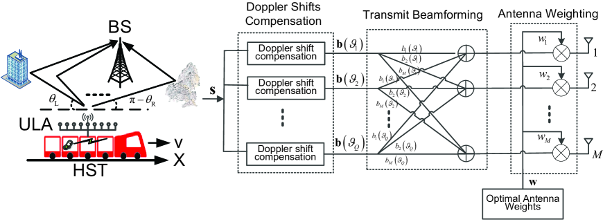
As illustrated in Fig. 1, we consider the high-mobility uplink transmission from a HST to BS, where an $M$-element ULA is equipped at HST. Denote the normalized antenna space of ULA as $d$, which is the ratio between the antenna space and the radio wavelength. Let the direction of ULA coincide with that of HST motion. We consider the flat fading channel for simplicity. Nevertheless, the proposed scheme can be directly applied to frequency selective channels. Specifically, the channel from HST to BS is composed of a bunch of propagation paths. We assume the angle of departure (AOD) of these paths is constrained within a region of $(\theta_{L},\theta_{R})$.

Denote ${{\bf s}}=[{s}(0),{s}(1),...,{s}(N-1)]^{T}$ as the length-$N$ transmitted time domain symbols in one orthogonal frequency division multiplexing (OFDM) block. We consider the antenna weighting technique [9] is adopted, where the $m\rm{th}$ antenna is weighted by a complex weight $w_{m}$. The multi-branch transmit matched filtering (MF) beamforming is performed towards a set of $Q$ selected directions ${{\vartheta}_{q}}\in({{\theta}_{L}},{{\theta}_{R}}),q=1,2,...,Q$. The $q$th MF beamformer is ${\bf b}({\vartheta_{q}})=\zeta\cdot{\rm{\bf a}(}{\vartheta_{q}}){e^{j\pi\phi_{q}}}$, where ${\bf a}(\vartheta_{q})=[1,{\rm e}^{j2\pi d\cos\vartheta_{q}},\cdots,{\rm e}^{j2\pi d(M-1)\cos\vartheta_{q}}]^{T}$ denotes the array response vector corresponding to direction $\vartheta_{q}$, $\zeta$ is the normalization coefficient to keep the total transmit power per symbol to 1 and $\phi_{q}$ denotes the introduced random phase.

Let ${\bf\Phi}(\epsilon)=\textrm{diag}(1,{\rm e}^{j\omega_{d}T_{s}\epsilon},\cdots,{\rm e}^{j\omega_{d}T_{s}(N-1)\epsilon})$ represent the $N\times N$ diagonal phase rotation matrix introduced by frequency shift of $f_{d}\epsilon$, with $\omega_{d}=2\pi f_{d}$ and $T_{s}$ being sampling interval. After transmit beamforming and Doppler shift compensation, the transmitted $M\times N$ signal matrix at transmit antenna array can be expressed as $\textrm{diag}({\bf w}){\bf b}^{*}({\vartheta_{q}}){\bf s}^{T}{\bf\Phi}(-\cos\vartheta_{q})$. ${\bf w}=[w_{1},w_{2},\cdots,w_{M}]^{T}$ denotes the weighting vector. Then, according to [9], the received signal at BS can be expressed in the form of

where $\alpha(\theta)$ represents the complex gain of the path associated with AOD $\theta$. Then, the equivalent uplink channel can be expressed as

where $G(\cos\theta,\cos\vartheta_{q})=\frac{1}{M}{\bf a}^{H}(\vartheta_{q})\textrm{diag}({\bf w}){\bf a}(\theta)$.

Assume that the directions are selected according to ‘Equi-cos’ criterion in [9] such that $\cos{\vartheta_{q}},q=1,2,...,Q$ are evenly distributed between $(\cos\theta_{R},\cos\theta_{L})$. According to [9], the channel PSD at BS can be expressed as $P(\omega)=\frac{1}{{{\omega_{d}}}}|{\mathcal{G}}(\tilde{\omega}){|^{2}}{W}(\tilde{\omega})$, where $\omega_{d}=2\pi f_{d}$ and $\tilde{\omega}={\frac{\omega}{{{\omega_{d}}}}}$ denotes the normalized Doppler frequency with respect to maximum Doppler shift. Denote ${\boldsymbol{\varsigma}}(\tilde{\omega})=[1,{\rm e}^{-j2\pi d\tilde{\omega}},\cdots,{\rm e}^{-j2\pi d(M-1)\tilde{\omega}}]^{T}$. Here, $|{\mathcal{G}}(\tilde{\omega}){|^{2}}$ and $W(\omega)$ are respectively named as beam function and window function, where $|{\mathcal{G}}(\tilde{\omega}){|^{2}}=|\frac{1}{M}{\boldsymbol{\varsigma}}^{T}(\tilde{\omega}){\bf w}{|^{2}}$ and

Afterwards, the Doppler spread with antenna weighting can be calculated as

where ${{\bf C}_{0}}=\int_{-\mu({\theta_{L}},{\theta_{R}})}^{\mu({\theta_{L}},{\theta_{R}})}{{W}(\tilde{\omega}){\boldsymbol{\varsigma}}^{*}(\tilde{\omega}){\boldsymbol{\varsigma}}^{T}(\tilde{\omega})d\tilde{\omega}}$, ${{\bf C}_{2}}=\int_{-\mu({\theta_{L}},{\theta_{R}})}^{\mu({\theta_{L}},{\theta_{R}})}{{{\tilde{\omega}}^{2}}}{W}(\tilde{\omega}){\boldsymbol{\varsigma}}^{*}(\tilde{\omega}){\boldsymbol{\varsigma}}^{T}(\tilde{\omega})d\tilde{\omega}$ and $\mu({\theta_{L}},{\theta_{R}})=\mathrm{cos}\theta_{L}-\mathrm{cos}\theta_{R}$.

Then, the normalized Doppler spread can be defined as

which represents the magnitude of Doppler spread suppression benefiting from the angle-domain Doppler shifts compensation scheme.

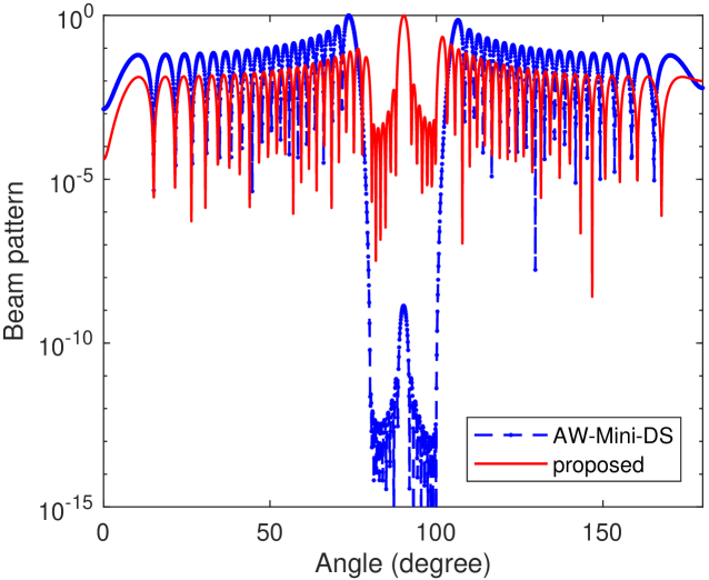
In the scheme in [9] (labelled as ‘AW-Mini-DS’), the antenna weighting is designed to only minimize the Doppler spread, which may lead to severe loss of transmission efficiency. Let us consider the following example. The AoDs are constrained within ($\theta_{L},\theta_{R}$) with $\theta_{L}=85^{\circ},\theta_{R}=95^{\circ}$. The ULA consists of $M=64$ antennas, the maximum Doppler shift is set as $f_{d}=5000$Hz, and the antenna spacing is taken as $d=0.45$. We depict the radiation pattern of the antenna array with the weighting technique in AW-Mini-DS in Fig. 2 by the solid line. It is evident that, in this case, although AW-Mini-DS can achieve the lowest Doppler spread, i.e., the smallest channel fluctuations, its radiation mainlobe is extremely lower than the sidelobes. This intuitively indicates that the vast majority of radiation power in AW-Mini-DS has leak out from the expected AoD region $(85^{\circ},95^{\circ})$.

More mathematically, it can be observed from [9] that, the total transmit signal power from antenna array can be expressed as ${{\bf w}^{H}}{\bf w}$, while ${{\bf w}^{H}}{\bf C}_{0}{\bf w}$ represents the magnitude of received signal power. Hence, we can define the energy radiation efficiency as $\frac{{{{\bf w}^{H}}{{\bf C}_{0}}{\bf w}}}{{{{\bf w}^{H}}{\bf w}}}$. The maximal energy radiation efficiency can be immediately obtained as $\lambda_{\max}({\bf C}_{0})$, which is the maximal eigenvalue of ${\bf C}_{0}$. Then, we further define the normalized energy radiation efficiency as

which is the ratio of the radiation efficiency to the maximum possible radiation efficiency and represents the level of maintained relative radiation efficiency. The normalized radiation efficiency equals $2\times 10^{-10}$ in AW-Mini-DS for the above example in Fig. 2, which means almost all of the radiation power has leaked out.

Based on the above observations, we propose a new antenna weighting scheme which targets at minimizing Doppler spread as well as maintaining the radiation efficiency. Given a minimal required normalized radiation efficiency $\varepsilon$, the optimization problem can be formulated as:

We can transfer the optimization problem (6) into

The detailed proof is omitted here due to the space limitation. Note that (7c) is a non-convex constraint. We then resort to the the SPCA method [11] to solve the above non-convex problem iteratively. Specifically, given the optimal solution in the $l\rm{th}$ iteration $\hat{\bf w}_{l}$, we know ${{\tilde{\bf w}}^{H}}{{\bf C}_{0}}{\tilde{\bf w}}$ is lower bounded by its first Taylor expansion $f(\tilde{\bf w},{\hat{\bf w}}_{l})$, where

Hence, the feasible set of $f(\tilde{\bf w},{\hat{\bf w}}_{l})\geq 1$ serves as a subset of the original constraint ${{\tilde{\bf w}}^{H}}{{\bf C}_{0}}{\tilde{\bf w}}\geq 1$. Then, the optimal solution in the $(l+1)\rm{th}$ iteration can be obtained by solving the following convex problem:

Note that the initial feasible solution $\hat{\bf w}_{0}$ can be found by the Iterative Feasibility Search Algorith (IFSA) algorithm [12]. In Fig. 2, we further include the radiation pattern of the proposed scheme with $\varepsilon=0.5$ for comparison. As expected, it is observed that the sidelobe level of the proposed scheme is much lower than that of AW-Mini-DS and the mainlobe level of the proposed scheme is much higher than that of AW-Mini-DS. This intuitively implies that the proposed method should provide much better radiation efficiency than AW-Mini-DS. More exactly, the normalized radiation efficiencies of the AW-Mini-DS and the proposed scheme in this example are $2\times 10^{-10}$ and $0.5$, respectively. In comparison, the corresponding normalized Doppler spreads are approximately given by $0.010$ and $0.012$, respectively. This verifies that the proposed scheme indeed could maintain radiation efficiency with slight sacrifice of Doppler spread suppression capability.

The massive MIMO system may suffer from high cost and complexity due to a large number of RF chains, making antenna selection urgently needed to reduce system complexity. In this section, we further exploit the idea of antenna selection for radiation efficiency aware Doppler spread suppression.

We consider that the $M$-element ULA of HST has at most $N$ RF chains ($N\leq M$). This is equivalent to impose an $l_{0}$-norm constraint on the weighting vector, that is $\|{\bf w}\|_{0}\leq N$. Here, $l_{0}$-norm $|\cdot|_{0}$ returns the number of non-zero elements of given argument. Especially, when $N\ll M$, the constraint of $\|{\bf w}\|_{0}\leq N$ implies that ${\bf w}$ is a sparse vector. Then, the antenna selection problem for radiation efficiency aware Doppler spread suppression can be formulated as:

Here, ${\bf C}_{0}(\tilde{\bf w})$ is a submatrix of ${\bf C}_{0}$ by deleting the column and row vectors corresponding to zero entries of trial weighting vector $\tilde{\bf w}$.

Bearing in mind that ${\bf C}_{0}(\tilde{\bf w})$ is parameterized by $\tilde{\bf w}$, directly solving the above problem (10) should be a nontrivial task. Next, we propose a two-step sub-optimal solution to the problem. The first step is to optimize the antenna selection for Doppler spread minimization without consideration of radiation efficiency. Once the antenna selection is determined, the radiation efficiency aware Doppler spread suppression scheme proposed in Section III can be immediately employed in the second step. Thus, in the following we will focus in the first step, which can be formulated as:

To circumvent the intractable non-convex problem (IV), we formulate the following function $S(\sigma)$:

The above problem (IV) tries to find the sparsest $\tilde{\bf w}$, given a maximal allowable Doppler spread $\sigma$. Moreover, the function $S(\sigma)$ is a decreasing function of the allowable Doppler spread $\sigma$. It can be observed that, the problem of (IV) is equivalent to solve the equation $S(\sigma)=N$. This can be solved efficiently via bisection method from an interval $[\sigma_{\min},\sigma_{\max}]$ with $S(\sigma_{\min})\geq N$ and $S(\sigma_{\max})\leq N$. Here, $\sigma_{\min}$ and $\sigma_{\max}$ can be set as the minimal Doppler spreads via AW-Mini-DS scheme with a fully connected $M$-element and $N$-element ULA, respectively.

Next, given a fixed $\sigma$, in order to solve the problem (IV), a good approach is to approximate the objective function by the well-known $l_{1}$-norm [10], that is

The above problem (IV) can be further transformed into

Similar to (7), the non-convex problem (14) can be iteratively solved by with the aid of SPCA method. In summary, the proposed antenna selection scheme in the first step can be described in table I.

In this section, we present simulation results to verify the proposed studies. We consider a ULA with a total of $M=64$ antennas and normalized antenna spacing of 0.45.

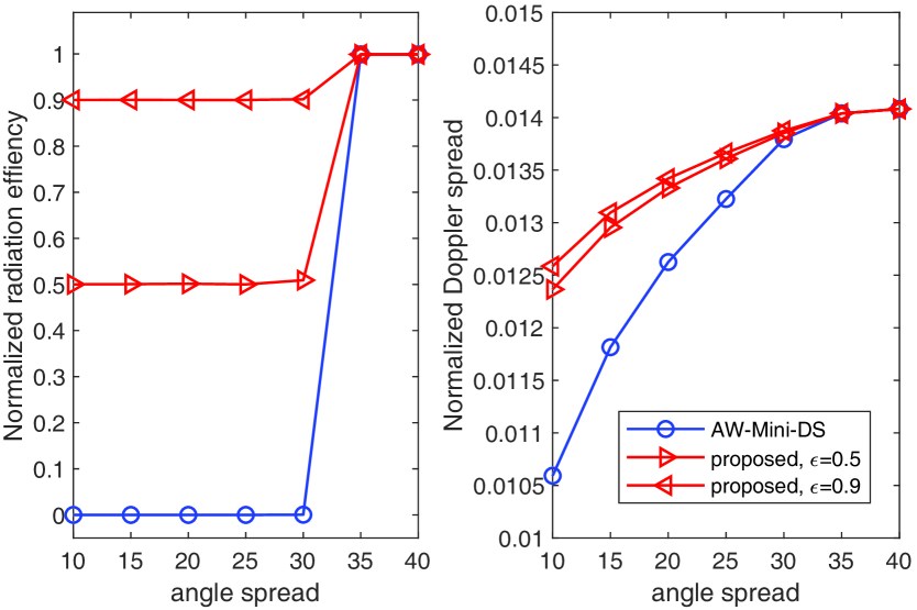
In the first example, we consider the case of fully connected ULA. We compare the performance between AW-Mini-DS and the proposed scheme in terms of both normalized radiation efficiency and Doppler spread as the angle spread $\theta_{R}-\theta_{L}$ increases in Fig. 3. The center AOD is fixed as $(\theta_{L}+\theta_{R})/2=90^{\circ}$. We can make the following observations: As the angle spread decreases, AW-Mini-DS can always provide the lowest Doppler spread (the best Doppler spread suppression). Unfortunately, the radiation efficiency of AW-Mini-DS quickly drops almost to zero once the angle spread becomes below $30^{\circ}$. In comparison, the results verify the effectiveness of the proposed radiation efficiency aware scheme. It is seen that, the proposed scheme could maintain the radiation efficiency according to the constraint $\varepsilon$ at the expense of slight Doppler spread suppression capability. Take the angle spread of $10^{\circ}$ as an example. As compared to AW-Mini-DS, the proposed scheme raises the Doppler spread by a factor of round $20\%$, but in the meanwhile improves the radiation efficiency from almost zero to 0.9. Hence, the proposed scheme has provided more balanced performance as compared to AW-Mini-DS.

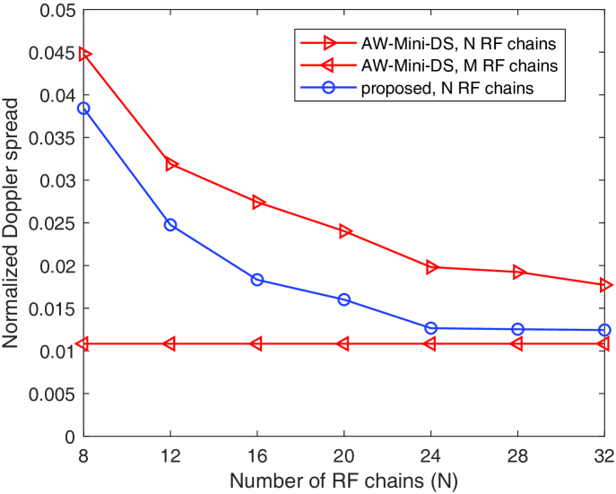
Next, we consider the case of partly connected ULA, where $M$-element ULA has at most $N$ RF chains. We display the evolution of normalized Doppler spread of the proposed antenna selection scheme as the number of RF chains increases in Fig. 4. We assume $\theta_{L}=30^{\circ}$ and $\theta_{R}=60^{\circ}$. For comparison, we also include the results of AW-Mini-DS in this figure. We consider that AW-Mini-DS employs the fully connected ULA with $N$ and $M$ RF chains, respectively. As expected, the AW-Mini-DS scheme with $N$ and $M$ RF chains serve as the upper and lower bound of the proposed scheme, respectively. With the same number of RF chains, the proposed scheme can greatly reduce the Doppler spread as compared to AW-Mini-DS. Moreover, as the number of RF chains increases, the proposed scheme could closely approach the lower bound, which demonstrates the effectiveness of the proposed antenna selection scheme.

In this paper, we considered the angle-domain Doppler shifts compensation scheme with maintaining radiation efficiency for high-mobility uplink communication. The idea of antenna selection is further exploited to reduce the number of required RF chains. Numerical results were provided to corroborate the proposed studies.

References

- [1] J. Wu, and P. Fan, “A survey on high mobility wireless communications: Challenges, opportunities and solutions,” IEEE Access, vol. 4, pp. 450-476, 2016.
- [2] T. Hwang, C. Yang, G. Wu, S. Li, and G. Y. Li, “OFDM and its wireless applications: A survey,” IEEE Trans. Veh. Technol., vol. 58, no. 4, pp. 1673-1694, May 2009.
- [3] Y. Zhang, Q. Yin, P. Mu, and L. Bai, “Multiple Doppler shifts compensation and ICI elimination by beamforming in high-mobility OFDM systems,” in Proc. Int. ICST Conf. Commun. and Netw. in China, Aug. 2011, pp. 170-175.
- [4] T. Marzetta, “Noncooperative cellular wireless with unlimited numbers of base station antennas,” IEEE Trans. Wirel. Commun., vol. 9, no. 11, pp. 3590-3600, Nov. 2010.
- [5] E. Larsson, O. Edfors, F. Tufvesson, and T. Marzetta, “Massive MIMO for next generation wireless systems,” IEEE Commun. Mag., vol. 52, no. 2, pp. 186-195, Feb. 2014.
- [6] W. Zhang, F. Gao, S. Jin, and H. Lin, “Frequency synchronization for uplink massive MIMO systems,” IEEE Trans. Wirel. Commun., vol. 17, no. 1, pp. 235-249, Jan. 2018.
- [7] W. Guo, W. Zhang, P. Mu and F. Gao, “High-Mobility OFDM Downlink Transmission With Large-Scale Antenna Array,” in IEEE Transactionson Vehicular Technology., vol. 66, no. 9, pp. 8600-8604, Sept. 2017.
- [8] W. Guo, W. Zhang, P. Mu, F. Gao, and B. Yao, “Angle-domain Doppler pre-compensation for high-mobility OFDM uplink with massive ULA,” in Proc. IEEE GLOBECOM, Dec. 2017, pp. 1-6.
- [9] Y. Ge, W. Zhang, F. Gao, S. Zhang, and X Ma, “Antenna Weighting for Reducing Channel Time Variation in High-Mobility Massive MIMO,” 2018. [Online]. Available: https://arxiv.org/abs/1809. 00137.
- [10] S. E. Nai, W. Ser, Z. L. Yu, and H. Chen, “Beampattern synthesis for linear and planar arrays with antenna selection by convex optimization, ” IEEE Trans. Ant. Propag., vol. 58, no. 12, pp. 3923-3930, Dec. 2010.
- [11] A. Beck, A. Ben-Tal, and L. Tetruashvili, “A sequential parametric convexapproximation method with applications to nonconvex truss topology design problems,” J. Global Optim., vol. 47, no. 1, pp. 29-51, May 2010.
- [12] Y. Cheng and M. Pesavento, “Joint optimization of source power allocation and distributed relay beamforming in multiuser peer-to-peer relay networks,” IEEE Trans. Signal Process., vol. 60, no. 6, pp. 2962-2973, Jun. 2012.