RANCOR: Non-Linear Image Registration with Total Variation Regularization

We propose a novel non-linear RegistrAtioN via COnvex Relaxation (RANCOR) algorithm that allows for the combination of any pointwise error metric (such as the sum of absolute intensity differences (SAD) for intra-modality registration, and mutual information (MI) [5, 6] or modality independent neighbourhood descriptors (MIND) [7] for inter-modality registration) while regularizing the deformation field by its total variation. This algorithm is implemented on GPGPU to ensure high performance.

Recent surveys provide a good overview of existing NLR registration methods [8, 9] and we would like to emphasize the study performed by Klein et al. [10], where 14 NLR registration algorithms were compared across four open brain image databases. We will compare our proposed method against the four highest ranked methods identified in [10]:

The first stage in our approach is the construction of the image pyramid. Let $I_{1}^{1}(x)$ …$I_{1}^{L}(x)$ be the $L$-level pyramid representation of $I_{1}(x)$ from the coarsest resolution $I_{1}^{1}(x)$ to the finest resolution $I_{1}^{L}(x)=I_{1}(x)$, and $I_{2}^{1}(x)$ …$I_{2}^{L}(x)$ the $L$-level coarse-to-fine pyramid representation of $I_{2}(x)$. The optimization process is started from the coarsest level, $\ell=1$, which extracts the deformation field $u^{1}(x)$ between $I_{1}^{1}(x)$ and $I_{2}^{1}(x)$ such that:

The vector field $u^{1}(x)$ gives the optimal deformation field at the coarsest scale. It is warped to the next finer-resolved level, $\ell=2$, to compute the optimal finer-level defomration field $u^{2}(x)$. The process is repeated, obtaining the deformation field $u^{3}(x)$ …$u^{L}(x)$ at each level sequentially.

Second, at each resolution level $\ell$, $\ell=2\ldots L$, we compute an incremental deformation field $t^{\ell}(x)$ based on the two image functions $I_{2}^{\ell}(x)$ and $I_{1}^{\ell}(x+u^{\ell-1})$, where $I_{1}^{\ell}(x+u^{\ell-1})$ is warped by the deformation field $u^{\ell-1}(x)$ computed at the previous resolution level $\ell-1$, i.e.

Clearly, the optimization problem (4) can be viewed as the special case of (5), i.e. for $\ell=1$, we define $u^{0}(x)=0$ and $u^{1}(x)=(u^{0}+t^{1})(x)$. Therefore, the proposed coarse-to-fine optimization framework sequentially explores the minimization of (5) at each image resolution level, from the coarsest $\ell=1$ to the finest $\ell=L$.

Now we consider the optimization problem (5) for each image resolution level $\ell$. Given the highly non-linear function $P(I_{1}^{\ell}(x+u^{\ell-1}),I_{2}^{\ell}(x);t^{\ell})$ in (5), we introduce a sequential linearization and convexification procedure for this challenging non-linear optimization problem (5). This results in a series of incremental warping steps in which each step approximates an update of the deformation field $t^{\ell}(x)=(t_{1}^{\ell}(x),t_{2}^{\ell}(x),t_{3}^{\ell}(x))^{\mbox{\tiny{T}}}$, until the updated deformation is sufficiently small, i.e., it iterates through the following sequence of convex minimization steps until convergence is attained:

• •

  Initialize $(h^{\ell})^{0}(x)=0$ and let $k=1$;

• •

  At the $k^{\text{th}}$ iteration, define the deformation field as

  $$\tilde{u}^{\ell-1}(x)\,:=\,\Big{(}u^{\ell-1}+\sum_{i=0}^{k-1}(h^{\ell})^{i}\Big{)}(x)$$

  and compute the update deformation $(h^{\ell})^{k}$ to $\tilde{u}^{\ell-1}(x)$ by minimizing the following convex energy function:

  $$\min_{(h^{\ell})^{k}}\;\int_{\Omega}\left\lvert\tilde{P}^{k}_{0}+\nabla\tilde{P}^{k}\cdot(h^{\ell})^{k}\right\rvert dx\,+\,R(u^{\ell-1}+(h^{\ell})^{k})\,,$$

  (6)

  where

  $$\tilde{P}^{k}((h^{\ell})^{k})\,=\,P(I_{1}^{\ell}(x+\tilde{u}^{\ell-1}),I_{2}^{\ell}(x);(h^{\ell})^{k})$$

  and $\tilde{P}_{0}^{k}(x)=P(I_{1}^{\ell}(x+\tilde{u}^{\ell-1}),I_{2}^{\ell}(x);0)$.

• •

  Let $k=k+1$ and repeat the second step till the new update $(h^{\ell})^{k}$ is small enough. Then, we have the total incremental deformation field $t^{\ell(x)}$ at the image resolution level $\ell$ as:

  $$t^{\ell}(x)\,=\,\sum_{i=0}^{k}(h^{\ell})^{i}(x)\,.$$

These steps can be viewed as a non-smooth GN method for the non-linear optimization problem (5), in contrast to the classical GN method proposed in [17]. Moreover, the $L_{1}$-norm and the convex regularization term $\mathcal{R}(\cdot)$, (6) results in a convex optimization problem. The non-smooth $L_{1}$-norm from (6) provides more robustness in practice than the conventional smooth $L_{2}$-norm used in the classical GN method.

Solving the convex minimization problem (6) is the most essential step in the proposed algorithmic framework The introduced primal-dual variational analysis not only provides an equivalent dual formulation to the optimization problem (6) but also derives an efficient solution algorithm. First, we simplify the expression of the convex problem (6) as:

where $\tilde{u}(x)$ represents the deformation field. Through variational analysis, we can derive an equivalent dual model to (7):

The proof is given in Appendix A.

As shown in Appendix A, each component of the deformation field $[h_{1}(x),h_{2}(x),h_{3}(x)]^{\mbox{\tiny{T}}}$ works as the optimal multiplier functions to their respective constraints, (9). Therfore, the energy function of the primal-dual model (24) is exactly the Lagrangian function to the dual model (8):

where $E(w,q)$ and the linear functions $F_{i}(x)$, $i=1,2,3$, are defined in (8) and (9) respectively. We can now derive an efficient duality-based Lagrangian augmented algorithm based on the modern convex optimization theories (see [18, 19, 20] for details), using the augmented Lagrangian function:

where $c>0$ is a positive constant and the additional quadratic penalty function is applied to ensure the functions (9) vanish. Our proposed duality-based optimization algorithm is:

• •

  Set the initial values of $w^{0}$, $q^{0}$ and $h^{0}$, and let $k=0$.

• •

  Fix $q^{k}$ and $h^{k}$, optimize $w^{k+1}$ by

  $\displaystyle w^{k+1}\,:=\,\arg\max_{\left\lvert w(x)\right\rvert\leq 1}\;L_{c}(h^{k},w,q^{k})\,$

  (11)

  generating the convex minimization problem:

  $\displaystyle\min_{\left\lvert w(x)\right\rvert\leq 1}\int wP_{0}dx+\frac{c}{2}\sum_{i=1}^{3}\int(w\partial_{i}P-T_{i}^{k})^{2}dx\,;$

  (12)

  where $T_{i}^{k}(x)$ ($i=1,2,3$) is computed from the fixed variables $q^{k}$ and $h^{k}$. $w^{k+1}$ is computed by threshholding:

  $\displaystyle w^{k+1}\,=\,\mathrm{Threshhold}_{\left\lvert w(x)\right\rvert\leq 1}(w^{k+1/2}(x))\,,$

  (13)

  where

  $$w^{k+1/2}\,=\,\frac{c\sum_{i=1}^{3}(\partial_{i}P\,\cdot T_{i}^{k})-P_{0}}{c\sum_{i=1}^{3}(\partial_{i}P)^{2}}\,.$$

• •

  Fixing $w^{k+1}$ and $h^{k}$, optimize $q^{k+1}$ by

  $\displaystyle q^{k+1}\,:=\,\arg\min_{q}\;L_{c}(h^{k},w^{k+1},q)\,;$

  (14)

  which amounts to three convex minimization problems:

  	$\displaystyle\min_{q_{i}}\,\int q_{i}\cdot\nabla\tilde{u}_{i}dx+\frac{c}{2}\int(\operatorname{div}q_{i}-U_{i}^{k})^{2}dx+R^{\ast}(q)\,;$
  	$\displaystyle i=1,2,3\,;$		(15)

  where $U_{i}^{k}$ is computed from the fixed variables $w^{k+1}$ and $h^{k}$. Hence, $q_{i}^{k+1}$, $i=1,2,3$, can be approximated by a gradient-projection step corresponding to (22).

• •

  Once $w^{k+1}$ and $q^{k+1}$ are obtained, update $h^{k+1}$ by

  	$\displaystyle h_{i}^{k+1}\,=\,h^{k}-c\Big{(}w^{k+1}\cdot\partial_{i}P+\operatorname{div}q_{i}^{k+1}\Big{)}\,;$
  	$\displaystyle i=1,2,3\,;$		(16)

• •

  Increment $k$ and iterate until converged, i.e.

  $\displaystyle c\int\left\lvert w^{k+1}\cdot\partial_{i}P+\operatorname{div}q_{i}^{k+1}\right\rvert dx\leq\delta\,,$

  (17)

  where $\delta$ is a chosen small positive parameter ($5\times 10^{-4}$).

The image data constisted of an open multi-center T1w MRI dataset with corresponding manual segmentations, the Internet Brain Segmentation Repository (IBSR) database, totalling 18 labeled image volumes at 1.5T available on www.mindboggle.info in a pre-processed form with labeling protocols and transforms into MNI space.

The experiments were performed in a pair-wise manner. For each image in the database, seventeen registrations were performed using the chosen image as the reference image and one of the remaining as the floating image. Thus, our experiment consisted of 306 registration problems in total.

Prior to registration, all images were skull stripped by constructing brain masks from manual labels using morphological operations [10] and then affinely registered using the FMRIB Software Library’s (FSL) FLIRT package [21] into the space of the MNI152_T1_1mm_brain. These affine transformations were made available on www.mindboggle.info and used to initialize the NLR algorithms. This guarantees that the same initialization is used for the algorithms in [10] and allows for quantitative comparisons. As a pre-processing step, both affinely registered images were robustly normalized to zero mean and standard deviation units to ensure a constant regularization weight $\alpha$ could be used.

The proposed NLR method was implemented in MATLAB (Natick, MA) using the Compute Unified Device Architecture (CUDA) (NVIDIA, Santa Clara, CA) for GPGPU computing. Each level in the coarse-to-fine framework constists of multiple warps invoking the proposed GPGPU accelerated regularization algorithm. Parameter tuning of the regularization weight $\alpha$ was done on two randomly picked dataset pairs similar to the tuning in [10]. All other parameters, such as the number of levels ($N_{Levels}$), the number of warps ($N_{Warps}$) and the maximum number of iterations ($It_{MAX}$) were determined heuristically on a single image volume not used in this study. Table 1 contains all set parameter values.

To compare our registration method against other NLR registration algorithms, we used the target overlap (TO) as a regional metric:

where $F$ is the floating image, $R$ the reference image, and $L$ a labeled region, as indicated in [10]. This parallels our motivation of using NLR registration to port segmentation labels to incoming datasets, and takes advantage of the manual segmentations providing in the IBSR database.

Results were considered significant if the probability of making a type I error was less than 1% ($p<0.01$). For this purpose, we employed a series of two-tailed, pairwise Student’s t-test.

The experiments were conducted on a Ubuntu 12.04 (64-bit) desktop machine with 144 GB memory and an NVIDIA Tesla C2060 (6 GB memory) graphics card. The maximum run times for the MATLAB code including pre-processing, optimization, and GPGPU enhanced regularization are given in Table 2.

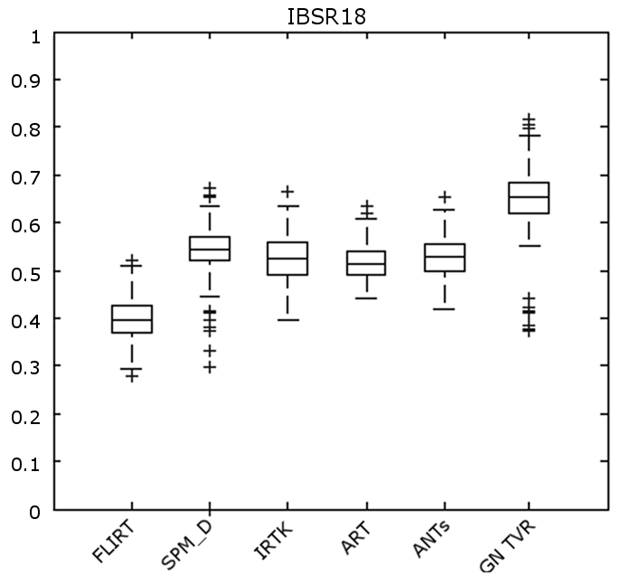
Figure 1 shows boxplots of the TO accuracy for each of the registration methods. The results were averaged across all regions. Numerical results are provided in Table 3.

The current RANCOR framework can be seen as a basic method to be extended over time, under the same open science credo, that allowed us to readily and quantitatively compare well-known open methods using public databases. As the current framework cannot currently guarantee diffeomorphic deformations, the next step is to enforce such constraints on the resulting deformation fields. Furthermore, to enable inter-modality NLR, we will implement and test commonly used advanced similarity metrics, such as normalized mutual-information, normalized cross-correlation, or more recently developed methods, such as the $L2-norm$ of the MIND descriptor [7]. Since command-line tools, such as the compared open NLR methods are needed for large-scale data analysis, RANCOR will be definitely included into such a package and, as a matter of course, be made available to the community.

Additionally, we plan to extend our evaluation to include the RANCOR algorithm under an $L2$-norm regularization as a substitute for total variation as used in Sun et al[22]. Such evaluation would allow for rigorous comparisons to be made by isolating the regularization mechanism.

References

- [1] M. Modat, G. R. Ridgway, Z. A. Taylor, M. Lehmann, J. Barnes, D. J. Hawkes, N. C. Fox, and S. Ourselin, “Fast free-form deformation using graphics processing units,” Computer methods and programs in biomedicine, vol. 98, no. 3, pp. 278–284, 2010.
- [2] M. Rajchl, J. Yuan, E. Ukwatta, and T. Peters, “Fast interactive multi-region cardiac segmentation with linearly ordered labels,” in Biomedical Imaging (ISBI), 2012 9th IEEE International Symposium on. IEEE Conference Publications, 2012, pp. Page–s.
- [3] W. Qiu, J. Yuan, E. Ukwatta, Y. Sun, M. Rajchl, and A. Fenster, “Fast globally optimal segmentation of 3d prostate mri with axial symmetry prior,” in Medical Image Computing and Computer-Assisted Intervention–MICCAI 2013. Springer Berlin Heidelberg, 2013, pp. 198–205.
- [4] M. Rajchl, J. Yuan, J. White, E. Ukwatta, J. Stirrat, C. Nambakhsh, F. Li, and T. Peters, “Interactive hierarchical max-flow segmentation of scar tissue from late-enhancement cardiac mr images,” IEEE Transactions on Medical Imaging, vol. 33, no. 1, pp. 159–172, 2014.
- [5] W. M. Wells III, P. Viola, H. Atsumi, S. Nakajima, and R. Kikinis, “Multi-modal volume registration by maximization of mutual information,” Medical image analysis, vol. 1, no. 1, pp. 35–51, 1996.
- [6] P. Rogelj, S. Kovačič, and J. C. Gee, “Point similarity measures for non-rigid registration of multi-modal data,” Computer vision and image understanding, vol. 92, no. 1, pp. 112–140, 2003.
- [7] M. P. Heinrich, M. Jenkinson, M. Bhushan, T. Matin, F. V. Gleeson, S. M. Brady, and J. A. Schnabel, “Mind: Modality independent neighbourhood descriptor for multi-modal deformable registration,” Medical Image Analysis, vol. 16, no. 7, pp. 1423–1435, 2012.
- [8] W. Crum, T. Hartkens, and D. Hill, “Non-rigid image registration: theory and practice,” 2004.
- [9] A. Gholipour, N. Kehtarnavaz, R. Briggs, M. Devous, and K. Gopinath, “Brain functional localization: a survey of image registration techniques,” Medical Imaging, IEEE Transactions on, vol. 26, no. 4, pp. 427–451, 2007.
- [10] A. Klein, J. Andersson, B. A. Ardekani, J. Ashburner, B. Avants, M.-C. Chiang, G. E. Christensen, D. L. Collins, J. Gee, P. Hellier et al., “Evaluation of 14 nonlinear deformation algorithms applied to human brain mri registration,” Neuroimage, vol. 46, no. 3, pp. 786–802, 2009.
- [11] B. B. Avants, C. L. Epstein, M. Grossman, and J. C. Gee, “Symmetric diffeomorphic image registration with cross-correlation: evaluating automated labeling of elderly and neurodegenerative brain,” Medical image analysis, vol. 12, no. 1, pp. 26–41, 2008.
- [12] K. Farahani, B. Menze, M. Reyes, E. Gerstner, J. Kirby, and J. Kalpathy-Cramer. (2013, Sep.) Multimodal brain tumor segmentation (brats 2013). [Online]. Available: http://martinos.org/qtim/miccai2013/index.html
- [13] K. Murphy, B. Van Ginneken, J. M. Reinhardt, S. Kabus, K. Ding, X. Deng, K. Cao, K. Du, G. E. Christensen, V. Garcia et al., “Evaluation of registration methods on thoracic ct: the empire10 challenge,” Medical Imaging, IEEE Transactions on, vol. 30, no. 11, pp. 1901–1920, 2011.
- [14] D. Rueckert, L. I. Sonoda, C. Hayes, D. L. Hill, M. O. Leach, and D. J. Hawkes, “Nonrigid registration using free-form deformations: application to breast mr images,” Medical Imaging, IEEE Transactions on, vol. 18, no. 8, pp. 712–721, 1999.
- [15] B. A. Ardekani, S. Guckemus, A. Bachman, M. J. Hoptman, M. Wojtaszek, and J. Nierenberg, “Quantitative comparison of algorithms for inter-subject registration of 3d volumetric brain mri scans,” Journal of neuroscience methods, vol. 142, no. 1, pp. 67–76, 2005.
- [16] J. Ashburner, “A fast diffeomorphic image registration algorithm,” Neuroimage, vol. 38, no. 1, pp. 95–113, 2007.
- [17] M. Baust, D. Zikic, N. Navab, and G. Munich, “Diffusion-based regularisation strategies for variational level set segmentation.” in BMVC, 2010, pp. 1–11.
- [18] D. P. Bertsekas, “Nonlinear programming,” 1999.
- [19] J. Yuan, E. Bae, and X.-C. Tai, “A study on continuous max-flow and min-cut approaches,” in Computer Vision and Pattern Recognition (CVPR), 2010 IEEE Conference on. IEEE, 2010, pp. 2217–2224.
- [20] J. Yuan, E. Bae, X.-C. Tai, and Y. Boykov, “A continuous max-flow approach to potts model,” in Computer Vision–ECCV 2010. Springer, 2010, pp. 379–392.
- [21] M. Jenkinson, P. Bannister, M. Brady, and S. Smith, “Improved optimization for the robust and accurate linear registration and motion correction of brain images,” Neuroimage, vol. 17, no. 2, pp. 825–841, 2002.
- [22] Y. Sun, J. Yuan, M. Rajchl, W. Qiu, C. Romagnoli, and A. Fenster, “Efficient convex optimization approach to 3d non-rigid mr-trus registration,” in Medical Image Computing and Computer-Assisted Intervention–MICCAI 2013. Springer, 2013, pp. 195–202.