This paper was converted on www.awesomepapers.org from LaTeX by an anonymous user.
Want to know more? Visit the Converter page.

Random Graph Matching in Geometric Models: the Case of Complete Graphs

Haoyu Wang, Yihong Wu, Jiaming Xu, and Israel Yolou H. Wang is with the Department of Mathematics, Yale University, New Haven, USA, haoyu.wang@yale.edu. Y. Wu is with the Department of Statistics and Data Science, Yale University, New Haven, USA, yihong.wu@yale.edu. J. Xu is with The Fuqua School of Business, Duke University, Durham NC, USA, jx77@duke.edu. I. Yolou is with the Departments of Mathematics and Computer Science, Yale University, New Haven, USA, israel.yolou@yale.edu.
Abstract

This paper studies the problem of matching two complete graphs with edge weights correlated through latent geometries, extending a recent line of research on random graph matching with independent edge weights to geometric models. Specifically, given a random permutation π\pi^{*} on [n][n] and nn iid pairs of correlated Gaussian vectors {Xπ(i),Yi}\{X_{\pi^{*}(i)},Y_{i}\} in d{\mathbb{R}}^{d} with noise parameter σ\sigma, the edge weights are given by Aij=κ(Xi,Xj)A_{ij}=\kappa(X_{i},X_{j}) and Bij=κ(Yi,Yj)B_{ij}=\kappa(Y_{i},Y_{j}) for some link function κ\kappa. The goal is to recover the hidden vertex correspondence π\pi^{*} based on the observation of AA and BB. We focus on the dot-product model with κ(x,y)=x,y\kappa(x,y)=\langle x,y\rangle and Euclidean distance model with κ(x,y)=xy2\kappa(x,y)=\|x-y\|^{2}, in the low-dimensional regime of d=o(logn)d=o(\log n) wherein the underlying geometric structures are most evident. We derive an approximate maximum likelihood estimator, which provably achieves, with high probability, perfect recovery of π\pi^{*} when σ=o(n2/d)\sigma=o(n^{-2/d}) and almost perfect recovery with a vanishing fraction of errors when σ=o(n1/d)\sigma=o(n^{-1/d}). Furthermore, these conditions are shown to be information-theoretically optimal even when the latent coordinates {Xi}\{X_{i}\} and {Yi}\{Y_{i}\} are observed, complementing the recent results of [DCK19] and [KNW22] in geometric models of the planted bipartite matching problem. As a side discovery, we show that the celebrated spectral algorithm of [Ume88] emerges as a further approximation to the maximum likelihood in the geometric model.

1 Introduction

Graph matching (or network alignment) refers to finding the best vertex correspondence between two graphs that maximizes the total number of common edges. While this problem, as an instance of quadratic assignment problem, is computationally intractable in the worst case, significant headways, both information-theoretic and algorithmic, have been achieved in the average-case analysis under meaningful statistical models [CK16, CK17, DMWX21, BCL+19, FMWX19a, FMWX19b, HM20, WXY21, GM20, GML22, MRT21b, MRT21a]. One of the most popular models is the correlated Erdős-Rényi graph model [PG11], where both observed graphs are Erdős-Rényi graphs with edges correlated through a latent vertex matching; more generally, in the correlated Wigner model, the observations are two weighted graph with correlated edge weights (e.g. Gaussians [DMWX21, DCK19, FMWX19a, Gan21a]). Despite their simplicity, these models inspired a number of new algorithms that achieve strong performance both theoretically and practically [DMWX21, FMWX19a, FMWX19b, GM20, GML22, MRT21b, MRT21a]. Nevertheless, one of the major limitations of models with independent edges is that they fail to capture graphs with spatial structure [AG14], such as those arising in computer vision datasets (e.g. mesh graphs obtained by triangulating 3D shapes [LRB+16]). In contrast to Erdős-Rényi-style model with iid edges, geometric graph models, such as random dot-product graphs and random geometric graphs, take into account the latent geometry by embedding each node in a Euclidean space and determines edge connection between two nodes by the proximity of their geographical location. While the coordinates are typically assumed to be independent (e.g. Gaussians or uniform over spheres or hypercubes), the edges or edge weights are now dependent. The main objective for the present paper is to study graph matching in correlated geometric graph models, where the network correlation is due to that of the latent coordinates.

1.1 Model

Given two point clouds {X1,,Xn}\{X_{1},\ldots,X_{n}\} and {Y1,,Yn}\{Y_{1},\ldots,Y_{n}\} in d{\mathbb{R}}^{d}, we construct two weighted graphs on the vertex set [n][n] with weighted adjacency matrices AA and BB as follows. For each i,ji,j, let AijindW(|Xi,Xj)A_{ij}\overset{\rm ind}{\sim}W(\cdot|X_{i},X_{j}) and BijindW(|Yi,Yj)B_{ij}\overset{\rm ind}{\sim}W(\cdot|Y_{i},Y_{j}), for some probability transition kernel WW. The coordinates are correlated through a latent matching as follows: Consider a Gaussian model

Yi=Xπ(i)+σZi,i=1,,n,Y_{i}=X_{\pi^{*}(i)}+\sigma Z_{i},\quad i=1,\ldots,n,

where Xi,ZiX_{i},Z_{i}’s are iid 𝒩(0,Id){\mathcal{N}}(0,I_{d}) vectors and π\pi^{*} is uniform on SnS_{n}, the set of all permutations on [n][n]. In matrix form, we have

Y=ΠX+σZ,Y=\Pi^{*}X+\sigma Z, (1)

where X,Y,Zn×dX,Y,Z\in\mathbb{R}^{n\times d} are matrices whose rows are XiX_{i}’s, YiY_{i}’s and ZiZ_{i}’s respectively, Π𝔖n\Pi^{*}\in\mathfrak{S}_{n} denotes the permutation matrix corresponding to π\pi^{*}, and 𝔖n\mathfrak{S}_{n} is the collection of all permutation matrices. Given the observation AA and BB, the goal is to recover the latent correspondence π\pi^{*}.

Of particular interest are the following special cases:

  • Dot-product model: The observations are complete graphs with pairwise inner products as edge weights, namely, Aij=Xi,XjA_{ij}=\langle X_{i},X_{j}\rangle and Bij=Yi,YjB_{ij}=\langle Y_{i},Y_{j}\rangle. As such, the weighted adjacency matrices are A=XXA=XX^{\top} and B=YYB=YY^{\top}, both Wishart matrices. It is clear that from AA and BB one can reconstruct XX and YY respectively, each up to a global orthogonal transformation on the rows. In this light, the model is also equivalent to the so-called Procrustes Matching problem [MDK+16, DL17, GJB19], where YY in (1) undergoes a further random orthogonal transformation – see Appendix A for a detailed discussion.

  • Distance model: The edge weights are pairwise squared distances Aij=XiXj2A_{ij}=\|X_{i}-X_{j}\|^{2} and Bij=XiXj2B_{ij}=\|X_{i}-X_{j}\|^{2}. This setting corresponds to the classical problem of multi-dimensional scaling (MDS), where the goal is to reconstruct the coordinates (up to global shift and orthogonal transformation) from the distance data (cf. [BG05]).

  • Random Dot Product Graph (RDPG): In this model, the observed data are two graphs with adjacency matrices AA and BB, where AijindBern(κ(Xi,Xj))A_{ij}\overset{\rm ind}{\sim}{\rm Bern}\left(\kappa(\left\langle X_{i},X_{j}\right\rangle)\right) and BijindBern(κ(Xi,Xj))B_{ij}\overset{\rm ind}{\sim}{\rm Bern}\left(\kappa(\left\langle X_{i},X_{j}\right\rangle)\right) conditioned on XX and YY, and κ:[0,1]\kappa:{\mathbb{R}}\to[0,1] is some link function, e.g. κ(t)=et2/2\kappa(t)=e^{-t^{2}/2}. In this way, we observe two instances of RDPG that are correlated through the underlying points and the latent matching. See [AFT+17] for a recent survey on RDPG.

  • Random Geometric Graph (RGG): Similar to RDPG, AijindBern(κ(XiXj))A_{ij}\overset{\rm ind}{\sim}{\rm Bern}(\kappa(\|X_{i}-X_{j}\|)) conditioned on X1,,XnX_{1},\ldots,X_{n} for some link function κ:+[0,1]\kappa:{\mathbb{R}}_{+}\to[0,1] applied to the pairwise distances. The second RGG instance BB is constructed in the same way using Y1,,YnY_{1},\ldots,Y_{n}. A simple example is κ(t)=𝟏{tr}\kappa(t)={\mathbf{1}_{\left\{{t\leq r}\right\}}} for some threshold r>0r>0, where each pair of points within distance rr is connected [Gil61]; see the monograph [Pen03] for a comprehensive discussion on RGG.

Linear assignmentmodel\begin{subarray}{c}\textrm{Linear assignment}\\ \textrm{model}\end{subarray}Dot productmodel\begin{subarray}{c}\textrm{Dot product}\\ \textrm{model}\end{subarray} Distance model\begin{subarray}{c}\textrm{~{}~{}Distance~{}~{}}\\ \textrm{model}\end{subarray}Random dot productgraph (RDPG)\begin{subarray}{c}\textrm{Random dot product}\\ \textrm{graph (RDPG)}\end{subarray}Random geometricgraph (RGG)\begin{subarray}{c}\textrm{Random geometric}\\ \textrm{graph (RGG)}\end{subarray}
Figure 1: Geometric matching models. Here arrows denote statistical ordering.

Let us mention that the model where the two point clouds are directly observed has been recently studied by [DCK19, DCK20] in the context of feature matching and independently by [KNW22] as a geometric model for the planted matching problem, extending the previous work in [CKK+10, MMX21, DWXY21] with iid weights to a geometric (low-rank) setting. In this model, XX and YY in (2) are observed and the maximum likelihood estimator (MLE) of π\pi^{*} amounts to solving

maxΠ𝔖nY,ΠX.\max_{\Pi\in\mathfrak{S}_{n}}\langle Y,\Pi X\rangle. (2)

which is a linear assignment (max-weight matching) problem on the weighted complete bipartite graph with weight matrix YXYX^{\top}. In the sequel we shall refer to this setting as the linear assignment model, which we also study in this paper for the sake of proving impossibility results for the more difficult graph matching problem, as the coordinates are latent and only pairwise information are available.

Fig. 1 elucidates the logical connections between the aforementioned models. Among these, linear assignment model is the most informative, followed by the dot product model and the distance model, whose further stochastically degraded versions are RDPG and RGG, respectively. As a first step towards understanding graph matching on geometric models, in this paper we study the case of weighted complete graphs in the dot product and distance models.

1.2 Main results

By analyzing the MLE (2) in the stronger linear assignment model (1), [KNW22] identified a critical scaling of dimension dd at logn\log n:

  • In the low-dimensional regime of dlognd\ll\log n, accurate reconstruction requires the noise level σ\sigma to be vanishingly small. More precisely, with high probability, the MLE (2) recovers the latent π\pi^{*} perfectly (resp. with a vanishing fraction of errors) provided that σ=o(n2/d)\sigma=o(n^{-2/d}) (resp. σ=o(n1/d)\sigma=o(n^{-1/d})).

  • In the high-dimensional regime of dlognd\gg\log n, it is possible for σ2\sigma^{2} to be as large as d(4+o(1))logn\frac{d}{(4+o(1))\log n}. Since the dependency between the edges weakens as the latent dimension increases,111For the Wishart matrix, it is known [JL15, BG18] that the total variation between the joint law of the off-diagonals and their iid Gaussian counterpart converges to zero provided that d=ω(n3)d=\omega(n^{3}). Analogous results have also been obtained in [BDER16] showing that high-dimensional RGG is approximately Erdős-Rényi. this is consistent with the known results in the correlated Erdős-Rényi and Wigner model. For example, to match two GOE matrices with correlation coefficient ρ\rho, the sharp reconstruction threshold is at ρ2=(4+o(1))lognn\rho^{2}=\frac{(4+o(1))\log n}{n} [Gan21b, WXY21].

In this paper we mostly focus on the low-dimensional setting as this is the regime where geometric graph ensembles are structurally distinct from Erdős-Rényi graphs. Our main findings are two-fold:

  1. 1.

    The same reconstruction thresholds remain achievable even when the coordinates are latent and only inner-product or distance data are accessible.

  2. 2.

    Furthermore, these thresholds cannot be improved even when the coordinates are observed.

To make these results precise, we start with the dot-product model with A=XXA=XX^{\top} and B=YYB=YY^{\top}, and Y=ΠX+σZY=\Pi^{*}X+\sigma Z according to (1). In this case the MLE turns out to be much more complicated than (2) for the linear assignment model. As shown in Appendix B, the MLE takes the form

Π^ML=argmaxΠ𝔖nO(d)dQexp(B1/2,ΠA1/2Qσ2),\widehat{\Pi}_{\mathrm{ML}}=\arg\max_{\Pi\in\mathfrak{S}_{n}}\int_{O(d)}{\rm d}Q\exp\left(\frac{\langle B^{1/2},\Pi A^{1/2}Q\rangle}{\sigma^{2}}\right), (3)

where the integral is with respect to the Haar measure on the orthogonal group O(d)O(d), A1/2UΛ1/2n×dA^{1/2}\triangleq U\Lambda^{1/2}\in{\mathbb{R}}^{n\times d} based on the SVD A=UΛUA=U\Lambda U^{\top}, and similarly for B1/2B^{1/2}. It is unclear whether the above Haar integral has a closed-form solution,222The integral in (3) can be reduced to computing dQexp(Λ,Q)\int{\rm d}Q\exp(\langle\Lambda,Q\rangle) for a diagonal Λ\Lambda, which, in principle, can be evaluated by Taylor expansion and applying formulas for the joint moments of QQ in [Mat13, Theorem 2.2]. let alone how to optimize it over all permutations. Next, we turn to its approximation.

As we will show later, in the low-dimensional case of d=o(logn)d=o(\log n), meaningful reconstruction of the latent matching is information-theoretically impossible unless σ\sigma vanishes with nn at a certain speed. In the regime of small σ\sigma, Laplace’s method suggests that the predominant contribution to the integral in (3) comes from the maximum B1/2,ΠA1/2Q\langle B^{1/2},\Pi A^{1/2}Q\rangle over QO(d)Q\in O(d). Using the dual form of the nuclear norm X=maxQO(d)X,Q\|X\|_{*}=\max_{Q\in O(d)}\langle X,Q\rangle, where X\|X\|_{*} denotes the sum of all singular values of XX, we arrive at the following approximate MLE:

Π^AML=argmaxΠ𝔖n(A1/2)ΠB1/2.\widehat{\Pi}_{\mathrm{AML}}=\arg\max_{\Pi\in\mathfrak{S}_{n}}\|(A^{1/2})^{\top}\Pi^{\top}B^{1/2}\|_{*}. (4)

We stress that the above approximation to the MLE (3) is justified for the low-dimensional regime where σ\sigma is small. In the high-dimensional (high-noise) case, the approximate MLE actually takes on the form of a quadratic assignment problem (QAP), which is the MLE for the well-studied iid model [CK16]; in the special case of the dot-product model, it amounts to replacing the nuclear norm in (4) by the Frobenius norm. We postpone this discussion to Section 4.

To measure the accuracy of a given estimator π^\widehat{\pi}, we define

𝗈𝗏𝖾𝗋𝗅𝖺𝗉(π^,π)1n|{i[n]:π^(i)=π(i)}|\mathsf{overlap}(\widehat{\pi},\pi)\triangleq\frac{1}{n}|\left\{i\in[n]:\widehat{\pi}(i)=\pi(i)\right\}|

as the fraction of nodes whose matching is correctly recovered. The following result identifies the threshold at which the approximate MLE achieves perfect or almost perfect recovery.

Theorem 1 (Recovery guarantee of AML in the dot-product model).

Assume the dot-product model with d=o(logn)d=o(\log n). Let π^AML\widehat{\pi}_{\mathrm{AML}} be the approximate MLE defined in (4).

  1. (i)

    If σn2/d\sigma\ll n^{-2/d}, the estimator π^AML\widehat{\pi}_{\mathrm{AML}} achieves perfect recovery with high probability:

    {𝗈𝗏𝖾𝗋𝗅𝖺𝗉(π^AML,π)=1}=1o(1).\mathbb{P}\left\{\mathsf{overlap}(\widehat{\pi}_{\mathrm{AML}},\pi^{*})=1\right\}=1-o(1). (5)
  2. (ii)

    If σn1/d\sigma\ll n^{-1/d}, the estimator π^AML\widehat{\pi}_{\mathrm{AML}} achieves almost perfect recovery with high probability:

    {𝗈𝗏𝖾𝗋𝗅𝖺𝗉(π^AML,π)1o(1)}=1o(1).\mathbb{P}\left\{\mathsf{overlap}(\widehat{\pi}_{\mathrm{AML}},\pi^{*})\geq 1-o(1)\right\}=1-o(1). (6)

A few remarks are in order:

  • In fact we will show the following nonasymptotic estimate that implies (6): For all sufficiently small ε\varepsilon, if σd>16n22/ε\sigma^{-d}>16n2^{2/\varepsilon}, then 𝗈𝗏𝖾𝗋𝗅𝖺𝗉(π^AML,π)1ε\mathsf{overlap}(\widehat{\pi}_{\mathrm{AML}},\pi^{*})\geq 1-\varepsilon with probability tending to one.

  • The estimator (4) has previously appeared in the literature of Procrustes matching [GJB19], albeit not as an approximation to the MLE in a generative model. See Appendix A for a detailed discussion.

  • Unlike linear assignment, it is unclear how to solve the optimization in (4) over permutations efficiently. Nevertheless, for constant dd we show that it is possible to find an approximate solution in time that is polynomial in nn that achieves the same statistical guarantee as in Theorem 1. Indeed, note that (3) is equivalent to the double maximization

    Π^AML=argmaxΠ𝔖nmaxQO(d)B1/2,ΠA1/2Q.\widehat{\Pi}_{\mathrm{AML}}=\arg\max_{\Pi\in\mathfrak{S}_{n}}\max_{Q\in O(d)}\langle B^{1/2},\Pi A^{1/2}Q\rangle. (7)

    Approximating the inner maximum over a suitable discretization of O(d)O(d), each maximization over Π\Pi for fixed QQ is a linear assignment problem, which can be solved in O(n3)O(n^{3}) time. In Section 3, we provide a heuristic that shows (7) can be further approximated by the classical spectral algorithm of Umeyama [Ume88] which is much faster in practice and achieves good empirical performance. For dd that grows with nn, it is an open question to find a polynomial-time algorithm that attains the (optimal, as we show next) threshold in Theorem 1.

Next, we proceed to the more difficult distance model, where Aij=XiXj2A_{ij}=\|X_{i}-X_{j}\|^{2} and Bij=YiYj2B_{ij}=\|Y_{i}-Y_{j}\|^{2}. Deriving the exact MLE in this model appears to be challenging; instead, we apply the estimator (4) to an appropriately centered version of the data matrices. Let 𝟏n\mathbf{1}\in{\mathbb{R}}^{n} denotes the all-one vector and define 𝐅=1n𝟏𝟏\mathbf{F}=\frac{1}{n}\mathbf{1}\mathbf{1}^{\top}. Then A=2XX+a𝟏+𝟏aA=-2XX^{\top}+a\mathbf{1}^{\top}+\mathbf{1}a^{\top} and B=2YY+b𝟏+𝟏bB=-2YY^{\top}+b\mathbf{1}^{\top}+\mathbf{1}b^{\top}, where a=(Xi2)a=(\|X_{i}\|^{2}) and b=(Yi2)b=(\|Y_{i}\|^{2}). Strictly speaking, the vectors aa and bb are correlated with the ground truth π\pi^{*}, since bb can be viewed as a noisy version of Πa\Pi^{*}a; however, we expect them to inform very little about π\pi^{*} because such scalar-valued observations are highly sensitive to noise (analogous to degree matching in correlated Erdős-Rényi graphs [DMWX21, Section 1.3]). As such, we ignore aa and bb by projecting AA and BB to the orthogonal complement of the vector 𝟏\mathbf{1}. Specifically, we compute, as commonly done in the MDS literature (see e.g. [SRZF03, OMK10]),

A~=12(I𝐅)A(I𝐅),B~=12(I𝐅)B(I𝐅).\widetilde{A}=-\frac{1}{2}(I-\mathbf{F})A(I-\mathbf{F}),\quad\widetilde{B}=-\frac{1}{2}(I-\mathbf{F})B(I-\mathbf{F}). (8)

It is easy to verify that A~=X~X~\widetilde{A}=\widetilde{X}\widetilde{X}^{\top} and B~=Y~Y~\widetilde{B}=\widetilde{Y}\widetilde{Y}^{\top}, where X~=(I𝐅)X\widetilde{X}=(I-\mathbf{F})X and Y~=(I𝐅)Y\widetilde{Y}=(I-\mathbf{F})Y consist of centered coordinates X~i=XiX¯\widetilde{X}_{i}=X_{i}-\bar{X} and Y~i=YiY¯\widetilde{Y}_{i}=Y_{i}-\bar{Y} respectively, with X¯=1ni=1nXi\bar{X}=\frac{1}{n}\sum_{i=1}^{n}X_{i} and Y¯=1ni=1nYi\bar{Y}=\frac{1}{n}\sum_{i=1}^{n}Y_{i}. Overall, we have reduced the distance model to a dot product model where the latent coordinates are now centered.

One can show that the MLE of Π\Pi^{*} given the reduced data (A~,B~)(\widetilde{A},\widetilde{B}) is of the same Haar-integral form (3). Using again the small-σ\sigma approximation, we arrive at the following estimator by applying (4) to the centered data A~\widetilde{A} and B~\widetilde{B}:

Π~AML=argmaxΠ𝔖n(A~1/2)ΠB~1/2.\widetilde{\Pi}_{\mathrm{AML}}=\arg\max_{\Pi\in\mathfrak{S}_{n}}\|(\widetilde{A}^{1/2})^{\top}\Pi^{\top}\widetilde{B}^{1/2}\|_{*}. (9)
Theorem 2 (Recovery guarantee in the distance model).

Assuming the distance model, Theorem 1 holds under the same condition on dd and σ\sigma, with the estimator Π~AML\widetilde{\Pi}_{\mathrm{AML}} in (9) replacing Π^AML\widehat{\Pi}_{\mathrm{AML}} in (4).

Finally, we state an impossibility result for the linear assignment model, proving that the perfect and almost perfect recovery threshold of σ=o(n2/d)\sigma=o(n^{-2/d}) and σ=o(n1/d)\sigma=o(n^{-1/d}) obtained by analyzing the MLE in [KNW22] are in fact information-theoretically necessary. Complementing Theorem 1 and Theorem 2, this result also establishes the optimality of the estimator (4) and (9) for their respective model.

Theorem 3 (Impossibility result in the linear assignment model).

Consider the linear assignment model with d=o(logn)d=o(\log n).

  1. (i)

    If there exists an estimator that achieves perfect recovery with high probability, then σn2/d\sigma\leq n^{-2/d}.

  2. (ii)

    If there exists an estimator that achieves almost perfect recovery with high probability, then σn(1o(1))/d\sigma\leq n^{-\left(1-o(1)\right)/d}.

Furthermore, in the special case of d=Θ(1)d=\Theta(1), necessary conditions in (i)(i) and (ii)(ii) can be improved to σo(n2/d)\sigma\leq o(n^{-2/d}) and σo(n1/d)\sigma\leq o(n^{-1/d}), respectively.

Theorem 3(i) slightly improves the necessary condition for perfect recovery in [KNW22] from σ=O(n2/d)\sigma=O(n^{-2/d}) to σ=o(n2/d)\sigma=o(n^{-2/d}). For almost perfect recovery, the negative result in [KNW22] is limited to MLE, while Theorem 3 holds for all algorithms. Moreover, the necessary condition in Theorem 3(ii) was conjectured in [KNW22, Conjecture 1.4, item 1], which we now resolve in the positive. Finally, while our focus is in the low-dimensional case of d=o(logn)d=o(\log n), we also provide necessary conditions that hold for general dd. (See Appendix E for details).

In view of Fig. 1, since the negative results in Theorem 3 are proved for the strongest model and the positive results in Theorem 2 are for the weakest model, we conclude that for all three models, namely, linear assignment, dot-product, and distance model, the thresholds for exact and almost perfect reconstruction is given by n2/dn^{-2/d} and n1/dn^{-1/d}, respectively.

2 Outline of proofs

2.1 Positive results

The positive results of Theorem 1 and Theorem 2 are proved in Appendix C and Appendix D. Here we briefly describe the proof strategy in the dot product model. Suppose we want to bound the probability that the approximate MLE Π^AML\widehat{\Pi}_{\mathrm{AML}} in (4) makes more than tt number of errors. Denote by d(π1,π2)i=1n𝟏{π1(i)π2(i)}{\rm d}(\pi_{1},\pi_{2})\triangleq\sum_{i=1}^{n}{\mathbf{1}_{\left\{{\pi_{1}(i)\neq\pi_{2}(i)}\right\}}} the Hamming distance between two permutations π1,π2Sn\pi_{1},\pi_{2}\in S_{n}. Without loss of generality, we will assume that π=Id\pi^{*}=\mathrm{Id}. By the orthogonal invariance of \|\cdot\|_{*}, we can assume, for the sake of analysis, that A1/2=XA^{1/2}=X and B1/2=YB^{1/2}=Y. Applying (7),

{d(Π^AML,Id)>t}\displaystyle\mathbb{P}\left\{{\rm d}(\widehat{\Pi}_{\mathrm{AML}},\mathrm{Id})>t\right\}\leq {maxπ:d(π,Id)>tXΠYXY}\displaystyle\mathbb{P}\left\{\max_{\pi:{\rm d}(\pi,\mathrm{Id})>t}\|X^{\top}\Pi^{\top}Y\|_{*}\geq\|X^{\top}Y\|_{*}\right\}
\displaystyle\leq {maxπ:d(π,Id)>tmaxQO(d)XΠY,QXY,Id}.\displaystyle\mathbb{P}\left\{\max_{\pi:{\rm d}(\pi,\mathrm{Id})>t}\max_{Q\in O(d)}\langle X^{\top}\Pi^{\top}Y,Q\rangle\geq\langle X^{\top}Y,I_{d}\rangle\right\}. (10)

For each fixed Π\Pi and QQ, averaging over the noise yields, for some absolute constant c0c_{0},

{XΠY,QXY,Id}𝔼exp{c0σ2XΠXQF2}.\mathbb{P}\left\{\langle X^{\top}\Pi^{\top}Y,Q\rangle\geq\langle X^{\top}Y,I_{d}\rangle\right\}\leq\mathbb{E}\exp\left\{-\frac{c_{0}}{\sigma^{2}}\left\|{X-\Pi XQ}\right\|_{{\rm F}}^{2}\right\}. (11)

In the remaining argument, there are three places where the structure of the orthogonal group O(d)O(d) plays a crucial role:

  1. 1.

    The quantity in (11) turns out to depend on Π\Pi through its cycle type and on QQ through its eigenvalues. Crucially, the eigenvalues of an orthogonal matrix QQ lie on the unit circle, denoted by (eiθ1,,eiθd)(e^{\mathrm{i}\theta_{1}},\ldots,e^{\mathrm{i}\theta_{d}}), with |θ|π|\theta_{\ell}|\leq\pi. We then show that the error probability in (11) can be further bounded by, for some absolute constant C0C_{0},

    (C0σ)d(n𝔠)(=1dC0σσ+|θ|)n1,(C_{0}\sigma)^{d(n-{\mathfrak{c}})}\left(\prod_{\ell=1}^{d}\frac{C_{0}\sigma}{\sigma+|\theta_{\ell}|}\right)^{n_{1}}, (12)

    where n1n_{1} is the number of fixed points in π\pi and 𝔠{\mathfrak{c}} is the total number of cycles.

  2. 2.

    In order to bound (10), we take a union bound over π\pi and another union bound over an appropriate discretization of O(d)O(d). This turns out to be much subtler than the usual δ\delta-net-based argument, as one needs to implement a localized covering and take into account the local geometry of the orthogonal group. Specifically, note that the error probability in (11) becomes larger when π\pi is near Id\mathrm{Id} and when QQ is near IdI_{d} (i.e. the phases |θ||\theta_{\ell}|’s are small); fortunately, the entropy (namely, the number of such π\pi and such QQ within a certain resolution) also becomes smaller, balancing out the deterioration in the probability bound. This is the second place where the structure of O(d)O(d) is used crucially, as the local metric entropy of O(d)O(d) in the vicinity of IdI_{d} is much lower than that elsewhere.

  3. 3.

    Controlling the approximation error of the nuclear norm is another key step. Note that for any matrix norm of the dual form A=supQ1A,Q\|A\|=\sup_{\|Q\|^{\prime}\leq 1}\langle A,Q\rangle, where \|\cdot\|^{\prime} is the dual norm of \|\cdot\|, the standard δ\delta-net argument (cf. [Ver18, Lemma 4.4.1]) yields a multiplicative approximation maxQNA,Q(1δ)A\max_{Q\in N}\left\langle A,Q\right\rangle\geq(1-\delta)\|A\|, where NN is any δ\delta-net of the dual norm ball. In general, this result cannot be improved (e.g. for Frobenius norm); nevertheless, for the special case of nuclear norm, this approximation ratio can be improved from 1δ1-\delta to 1δ21-\delta^{2}, as the following result of independent interest shows. This improvement turns out to be crucial for obtaining the sharp threshold.

    Lemma 1.

    Let NO(d)N\subset O(d) be a δ\delta-net in operator norm of the orthogonal group O(d)O(d). For any Ad×dA\in\mathbb{R}^{d\times d},

    maxQNA,Q(1δ22)A.\max_{Q\in N}\left\langle A,Q\right\rangle\geq\left(1-\frac{\delta^{2}}{2}\right)\|A\|_{*}. (13)

The proof of Theorem 1 is completed by combining (12) with a union bound over a specific discretization of O(d)O(d), whose cardinality satisfies the desired eigenvalue-based local entropy estimate, followed by a union bound over π\pi which can be controlled using moment generating function of the number of cycles in a random derangement.

2.2 Negative results

The information-theoretic lower bounds in Theorem 3 for the linear assignment model are proved in Appendix E. Here we sketch the main ideas. We first derive a necessary condition for almost perfect recovery that holds for any dd via a simple mutual information argument [HWX17]: On one hand, the mutual information I(π;X,Y)I(\pi^{*};X,Y) can be upper bounded by the Gaussian channel capacity as nd2log(1+σ2)\frac{nd}{2}\log(1+\sigma^{-2}). On the other hand, to achieve almost perfect recovery, I(π;X,Y)I(\pi^{*};X,Y) needs be asymptotically equal to the full entropy H(π)H(\pi^{*}) which is (1o(1))logn(1-o(1))\log n. These two assertions together immediately imply that nd2log(1+σ2)((1o(1))logn\frac{nd}{2}\log(1+\sigma^{-2})\geq((1-o(1))\log n, which further simplifies to σ=n(1o(1))/d\sigma=n^{-(1-o(1))/d} when d=o(logn)d=o(\log n). However, for constant dd, this necessary condition turns out to be loose and the main bulk of our proof is to improve it to the optimal condition σ=o(n1/d)\sigma=o(n^{-1/d}). To this end, we follow the program recently developed in [DWXY21] in the context of the planted matching model by analyzing the posterior measure of the latent π\pi^{*} given the data (X,Y)(X,Y).

To start, a simple yet crucial observation in [DWXY21] is that to prove the impossibility of almost perfect recovery, it suffices to show a random permutation sampled from the posterior distribution is at Hamming distance Ω(n)\Omega(n) away from the ground truth with constant probability. As such, it suffices to show there is more posterior mass over the bad permutations (those far away from the ground truth) than that over the good permutations (those near the ground truth) in the posterior distribution. To proceed, we first bound from above the total posterior mass of good permutations by a truncated first moment calculation applying the large deviation analysis developed in the proof of the positive results. To bound from below the posterior mass of bad permutations, we aim to construct exponentially many bad permutations π\pi whose log likelihood L(π)L(\pi) is no smaller than L(π)L(\pi^{*}). A key observation is that L(π)L(π)L(\pi)-L(\pi^{*}) can be decomposed according to the orbit decomposition of (π)1π(\pi^{*})^{-1}\circ\pi:

L(π)L(π)=1σ2ΠXΠX,Y=1σ2O𝒪Δ(O),\displaystyle L(\pi)-L(\pi^{*})=\frac{1}{\sigma^{2}}\left\langle\Pi X-\Pi^{*}X,Y\right\rangle=\frac{1}{\sigma^{2}}\sum_{O\in{\mathcal{O}}}\Delta(O), (14)

where 𝒪{\mathcal{O}} denotes the set of orbits in (π)1π(\pi^{*})^{-1}\circ\pi and for any orbit O=(i1,i2,,it)O=(i_{1},i_{2},\ldots,i_{t}),

Δ(O)k=1tXπ(ik+1)Xπ(ik),Yik.\displaystyle\Delta(O)\triangleq\sum_{k=1}^{t}\left\langle X_{\pi^{*}(i_{k+1})}-X_{\pi^{*}(i_{k})},Y_{i_{k}}\right\rangle. (15)

Thus, the goal is to find a collection of vertex-disjoint orbits OO whose total lengths add up to Ω(n)\Omega(n) and each of which is augmenting in the sense that Δ(O)0\Delta(O)\geq 0. Here, a key difference to [DWXY21] is that in the planted matching model with independent edge weights studied there, short augmenting orbits are insufficient to meet the Ω(n)\Omega(n) total length requirement; instead, [DWXY21] resorts to a sophisticated two-stage process that first finds many augmenting paths then connects then into long cycles. Fortunately, for the linear assignment model in low dimensions of d=Θ(1)d=\Theta(1), as also observed in [KNW22] in their analysis of the MLE, it suffices to look for augmenting 22-orbits and take their disjoint unions. More precisely, we show that there are Ω(n)\Omega(n) many vertex-disjoint augmenting 22-orbits. This has already been done in [KNW22] using a second-moment method enhanced by an additional concentration inequality. It turns out that the correlation among the augmenting 22-orbits is mild enough so that a much simpler argument via a basic second-moment calculation followed by an application of Turán’s theorem suffices to extract a large vertex-disjoint subcollection. Finally, these vertex-disjoint augmenting 22-orbits give rise to exponentially many permutations that differ from the ground truth by Ω(n)\Omega(n).

Finally, we briefly remark on perfect recovery, for which it suffices to focus on the MLE (2) which minimizes the error probability for uniform π\pi^{*}. In view of the likelihood decomposition given in (14), it further suffices to prove the existence of an augmenting 22-orbit. This can be easily done using the second-moment method. A similar strategy was adopted in [DCK19], but our first-moment and second-moment estimates are tighter and hence yield nearly optimal conditions.

3 Experiments

In this section we present preliminary numerical results on synthetic data from the dot product model. As observed in [GJB19], the form of the approximate MLE Π^AML\widehat{\Pi}_{\mathrm{AML}} in (7) as a double maximization over Π𝔖n\Pi\in\mathfrak{S}_{n} and QO(d)Q\in O(d) naturally suggests an alternating maximization strategy by iterating between the two steps: (a) For a fixed QQ, the Π\Pi-maximization is a linear assignment; (b) For a fixed Π\Pi, the QQ-maximization is the so-called orthogonal Procrustes problem and easily solved via SVD [Sch66]. However, with random initialization this method performs rather poorly falling short of the optimal threshold predicted by Theorem 1. While more informative initialization (such as starting from a Π\Pi obtained by the doubly-stochastic relaxation of QAP [GJB19]) can potentially help, in this section we focus on methods that are closer to the original approximate MLE.

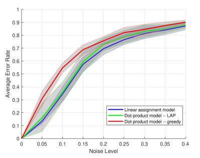
As the proof of Theorem 1 shows, as far as achieving the optimal threshold is concerned it suffices to consider a finely discretized O(d)O(d). This can be easily implemented in d=2d=2, since any 2×22\times 2 orthogonal matrix is either a rotation or reflection of the form: (cos(θ)sin(θ)sin(θ)cos(θ))\big{(}\begin{smallmatrix}\cos(\theta)&-\sin(\theta)\\ \sin(\theta)&\cos(\theta)\end{smallmatrix}\big{)} or (cos(θ)sin(θ)sin(θ)cos(θ))\big{(}\begin{smallmatrix}\cos(\theta)&\sin(\theta)\\ \sin(\theta)&-\cos(\theta)\end{smallmatrix}\big{)}. We then solve (7) on a grid of θ\theta values, by solving the Π\Pi-maximization for each such QQ and reporting the solution with the highest objective value. As shown in Fig. 2(a) for n=200n=200, the performance of the approximate MLE in the dot-product model (green) follows closely that of the MLE in the linear assignment model (blue). Using the greedy matching algorithm (red) in place of the linear assignment solver greatly speeds up the computation at the price of some performance degradation.

Refer to caption
(a) n=200n=200 and d=2d=2. The green and red curves correspond to (7) on T0=100T_{0}=100 discretized angles, with exact linear assignment or greedy matching.
Refer to caption
(b) n=200n=200 and d=4d=4. The green and red curves are based on (17) with exact linear assignment or greedy matching, and the yellow curve corresponds to the Umeyama algorithm (18).
Figure 2: Comparison of dot product model and linear assignment model (averaged over 10 random instances). In the latter, the blue curve corresponds to the MLE (2).

As the dimension increases, it becomes more difficult and computationally more expensive to discretize O(d)O(d). Instead, we take a different approach. Note that in the noiseless case (Y=ΠXY=\Pi^{*}X), as long as all singular values have multiplicity one, we have B1/2=ΠA1/2QB^{1/2}=\Pi^{*}A^{1/2}Q for some QQ in

2d={𝖽𝗂𝖺𝗀(qi):qi{±1}}.{\mathbb{Z}}_{2}^{\otimes d}=\{\mathsf{diag}(q_{i}):q_{i}\in\{\pm 1\}\}. (16)

As such, in the noiseless case it suffices to restrict the inner maximization of (7) to the subgroup 2d{\mathbb{Z}}_{2}^{\otimes d} corresponding to coordinate reflections. Since the noise is weak in the low-dimensional setting, we continue to apply this heuristic by computing

Π^AML,2d=argmaxΠ𝔖nmaxQ2dB1/2,ΠA1/2Q,\widehat{\Pi}_{\mathrm{AML},{\mathbb{Z}}_{2}^{\otimes d}}=\arg\max_{\Pi\in\mathfrak{S}_{n}}\max_{Q\in{\mathbb{Z}}_{2}^{\otimes d}}\langle B^{1/2},\Pi A^{1/2}Q\rangle, (17)

which turns out to work very well in practice. Taking this method one step further, notice that in the low-dimensional regime, all non-zero singular values of XX and YY are tightly concentrated on the same value n\sqrt{n}. If we ignore the singular values and simply replace A1/2A^{1/2} and B1/2B^{1/2} by their left singular vectors U=[u1,,ud]U=[u_{1},\ldots,u_{d}] and V=[v1,,vd]V=[v_{1},\ldots,v_{d}], (17) can be written more explicitly as

Π^Umeyama=argmaxΠ𝔖nmaxq{±1}dΠ,i=1dqiviui,\widehat{\Pi}_{\mathrm{Umeyama}}=\arg\max_{\Pi\in\mathfrak{S}_{n}}\max_{q\in\{\pm 1\}^{d}}\left\langle\Pi,\sum_{i=1}^{d}q_{i}v_{i}u_{i}^{\top}\right\rangle, (18)

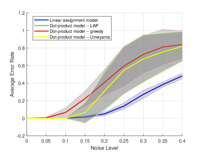
which, somewhat unexpectedly, coincides with the celebrated Umeyama algorithm [Ume88], a specific type of spectral method that is widely used in practice for graph matching. In Fig. 2(b) we compare for n=200n=200 and d=4d=4. Consistent with Theorem 1, the error rates in the dot-product model and the linear assignment model are both near zero until σ\sigma exceeds a certain threshold, after which the former departs from the latter. Finally, comparing Fig. 2(a) and Fig. 2(b) confirms that the reconstruction threshold improves as the latent dimension increases as predicted by Theorem 1.

4 Discussion

In this paper we studied the problem of graph matching in the special case of correlated complete weighted graphs in the dot product and distance model, as a first step towards the more challenging case of random dot-product graphs and random geometric graphs. Within the confines of the present paper, there still remain a number of interesting directions and open problems which we discuss below.

Non-isotropic distribution

The present paper assumes the latent coordinates XiX_{i}’s and YiY_{i}’s are isotropic Gaussians. For the linear assignment model, [DCK19, DCK20] has considered a more general setup where Xii.i.d.N(0,Σ)X_{i}{\stackrel{{\scriptstyle\text{i.i.d.}}}{{\sim}}}N(0,\Sigma) for some covariance matrix Σ\Sigma. As explained in [DCK19, Appendix A], it is not hard to see, based on a simple reduction argument (by scaling both XiX_{i}’s and YiY_{i}’s with Σ1/2\Sigma^{1/2} and add noise if needed), that as long as the singular values of Σ\Sigma are bounded from above and below, the information-theoretic limits in terms of σ\sigma remain unchanged. For the dot product or distance model, this is also true but less obvious – see Appendix F for a proof.

While the statistical limits in the nonisotropic case remain the same, potentially it allows more computationally tractable algorithms to succeed. For example, the spectral method recently proposed in [FMWX19a, FMWX19b] finds a matching by rounding the so-called GRAMPA similarity matrix

X=i,j=1nui,𝟏vj,𝟏(λiμj)2+η2uivj.X=\sum_{i,j=1}^{n}\frac{\langle u_{i},\mathbf{1}\rangle\langle v_{j},\mathbf{1}\rangle}{(\lambda_{i}-\mu_{j})^{2}+\eta^{2}}u_{i}v_{j}^{\top}. (19)

Here A=λiuiuiA=\sum\lambda_{i}u_{i}u_{i}^{\top} and B=μjvjvjB=\sum\mu_{j}v_{j}v_{j}^{\top} are the SVD of the observed weighted adjacency matrices, and η\eta is a small regularization parameter. In the isotropic case, applying this algorithm to the dot-product model is unlikely to achieve the optimal threshold in Theorem 1. The reason is that in the low-dimensional regime of small dd, both AA and BB and rank-dd and all singular values λi\lambda_{i}’s and μj\mu_{j}’s are largely concentrated on the same value of n\sqrt{n}. As such, the similarity matrix (19) degenerates into X1nη2i,j=1nλiμjui,𝟏vj,𝟏uivjabX\approx\frac{1}{n\eta^{2}}\sum_{i,j=1}^{n}\lambda_{i}\mu_{j}\langle u_{i},\mathbf{1}\rangle\langle v_{j},\mathbf{1}\rangle u_{i}v_{j}^{\top}\propto ab^{\top}, where a=A𝟏a=A\mathbf{1} and b=B𝟏b=B\mathbf{1} are the row-sum vectors. Rounding abab^{\top} to a permutation matrix is equivalent to “degree-matching”, that is, finding the permutation by sorting aa and bb, which can only tolerate σ=nc\sigma=n^{-c} type of noise level, for constant cc independent of the dimension dd, due to the small spacing in the order statistics [DMWX21]. However, in the nonisotropic case where Σ\Sigma has distinct singular values, we expect AA and BB to have descent spectral gaps and the spectral method (19) may succeed at the dimension-dependent thresholds of Theorem 1. A theoretical justification of this heuristic is outside the scope of this paper.

High-dimensional regime

Recall the exact MLE (3), wherein the objective function is an average over the Haar measure on O(d)O(d), can be approximated by (4) for small σ\sigma. Next, we derive its large-σ\sigma approximation. Rewriting the objective function in (3) as 𝔼[exp(1σ2B1/2,ΠA1/2𝐐)]\mathbb{E}[\exp(\frac{1}{\sigma^{2}}\langle B^{1/2},\Pi A^{1/2}\mathbf{Q}\rangle)] for a random uniform 𝐐O(d)\mathbf{Q}\in O(d) and taking its second-order Taylor expansion for large σ\sigma, we get

𝔼[exp(1σ2B1/2,ΠA1/2𝐐)]=1+12dσ4B,ΠAΠ+o(σ4),\mathbb{E}\left[\exp\left(\frac{1}{\sigma^{2}}\langle B^{1/2},\Pi A^{1/2}\mathbf{Q}\rangle\right)\right]=1+\frac{1}{2d\sigma^{4}}\langle B,\Pi A\Pi^{\top}\rangle+o(\sigma^{-4}),

where we applied 𝔼[𝐐,X]=0\mathbb{E}[\langle\mathbf{Q},X\rangle]=0, 𝔼[𝐐,X2]=XF2/d\mathbb{E}[\langle\mathbf{Q},X\rangle^{2}]=\left\|{X}\right\|_{{\rm F}}^{2}/d, and (A1/2)ΠB1/2F2=B,ΠAΠ\|(A^{1/2})^{\top}\Pi^{\top}B^{1/2}\|_{\rm F}^{2}=\langle B,\Pi A\Pi^{\top}\rangle. This expansion suggests that for large σ\sigma (which can be afforded in the high-dimensional regime of dlognd\gg\log n), the MLE is approximated by the solution to the following QAP:

Π^QAP=argmaxΠ𝔖nB,ΠAΠ.\widehat{\Pi}_{\mathrm{QAP}}=\arg\max_{\Pi\in\mathfrak{S}_{n}}\langle B,\Pi A\Pi^{\top}\rangle. (20)

This observation aligns with the better studied correlated Erdős-Rényi models or correlated Gaussian Wigner models, where the MLE is exactly given by the QAP (20).

To further compare with the estimator (4) that has been shown optimal in low dimensions, let us rewrite (20) in a form that parallels (7):

Π^QAP=argmaxΠ𝔖n(A1/2)ΠB1/2F=argmaxΠ𝔖nmaxQF1B1/2,ΠA1/2Q.\widehat{\Pi}_{\mathrm{QAP}}=\arg\max_{\Pi\in\mathfrak{S}_{n}}\|(A^{1/2})^{\top}\Pi^{\top}B^{1/2}\|_{\rm F}=\arg\max_{\Pi\in\mathfrak{S}_{n}}\max_{\|Q\|_{\rm F}\leq 1}\langle B^{1/2},\Pi A^{1/2}Q\rangle. (21)

In contrast, the dual variable QQ in (7) is constrained to be an orthogonal matrix, which, as discussed in the proof sketch in Section 2.1, is crucial for the proof of Theorem 1. Overall, the above evidence points to the potential suboptimality of QAP in low and moderate-dimensional regime of dlognd\lesssim\log n and its potential optimality in the high-dimensional regime of dlognd\gg\log n.

Practical algorithms

As demonstrated by extensive numerical experiments in [FMWX19a, Sec. 4.2], for correlated random graph models with iid pairs of edge weights, the Umeyama algorithm (18) significantly improves over classical “low-rank” spectral methods involving only the top few eigenvectors, but still lags behind the more recent spectral methods such as the GRAMPA algorithm (19) that uses all pairs of eigenvalues and eigenvectors. Surprisingly, in the low-dimensional dot product model with d=o(logn)d=o(\log n), while the GRAMPA algorithm is expected to perform poorly, empirical result in Section 3 indicates that the Umeyama method actually works very well in this setting. In fact, it is not hard to show that the Umeyama algorithm returns the true permutation with high probability in the noiseless case of σ=0\sigma=0; however, understanding its theoretical performance in the noisy setting remains open.

Appendix A Further related work

The present paper bridges several streams of literature such as planted matching, feature matching, Procrustes matching, and graph matching, which we describe below.

Planted matching and feature matching

The planted matching problem aims to recover a perfect matching hidden in a weighted complete n×nn\times n bipartite graph, where the edge weights are independently drawn from either 𝒫{\mathcal{P}} or 𝒬{\mathcal{Q}} depending on whether edges are on the hidden matching or not. Originally proposed by [CKK+10] to model the application of object tracking, a sharp phase transition from almost perfect recovery to partial recovery is conjectured to exist for the special case where 𝒫{\mathcal{P}} is a folded Gaussian and 𝒬{\mathcal{Q}} is a uniform distribution over [0,n][0,n]. A recent line of work initiated by [MMX21] and followed by [SSZ20, DWXY21] has successfully resolved the conjecture and characterized the sharp threshold for general distributions.

Despite these fascinating advances, they crucially rely on the independent weight assumption which does not account for the latent geometry in the object tracking applications. As a remedy, the linear assignment model (1) was proposed and studied by [KNW22] as a geometric model for planted matching, where the edge weights are pairwise inner products and no longer independent. In the low-dimensional setting of d=o(logn)d=o(\log n), the MLE is shown to achieve perfect recovery when σ=o(n2/d)\sigma=o(n^{-2/d}) and almost perfect recovery when σ=o(n1/d)\sigma=o(n^{-1/d}). Further bounds on the number of errors made by MLE and recovery guarantees in the high-dimensional setting are provided. However, the necessary conditions derived in [KNW22] only pertain to the MLE, leaving open the possibility that almost perfect recovery might be attained by other algorithms at lower threshold. This is resolved in the negative by the information-theoretic converse in Theorem 3, showing that σ=o(n1/d)\sigma=o(n^{-1/d}) is necessary for any algorithm to achieve almost perfect recovery. Along the way, we also slightly improve the necessary condition for perfect recovery from σ=O(n2/d)\sigma=O(n^{-2/d}) to σ=o(n2/d)\sigma=o(n^{-2/d}).

The linear assignment model (1) was in fact studied earlier in [DCK19, DCK20] in a different context of feature matching, where XiX_{i}’s and YiY_{i}’s are viewed as two correlated Gaussian feature vectors in d{\mathbb{R}}^{d} and the goal is to find their best alignment. It is shown in [DCK19] that perfect recovery is possible when d4log(1+σ2)logn+\frac{d}{4}\log\left(1+\sigma^{-2}\right)-\log n\to+\infty, and impossible when d4log(1+σ2)(1Ω(1))logn\frac{d}{4}\log\left(1+\sigma^{-2}\right)\leq(1-\Omega(1))\log n and 1d=O(logn)1\ll d=O(\log n).333While the impossibility result in [DCK19, Theorem 2] only states the assumption that d1d\gg 1, its proof, specifically the proof of [DCK19, Lemma 4.5], implicitly assumes σ=O(1)\sigma=O(1) which further implies d=O(logn)d=O(\log n). In comparison, the necessary condition in Theorem 5 is tighter and holds for any dd, agreeing with their sufficient condition within an additive logd\log d factor. It is also shown in [DCK20] that almost perfect recovery is possible when d2log(1+σ2)(1+ϵ)logn\frac{d}{2}\log\left(1+\sigma^{-2}\right)\geq(1+\epsilon)\log n in the high-dimensional regime d=ω(logn)d=\omega(\log n) for a small constant ϵ>0\epsilon>0. This matches our necessary condition in Proposition 1 with a sharp constant.

Related problems on feature matching were also studied in the statistics literature. For example, [CD16] studies the model of observing Y=X+σZY=X+\sigma Z and Y=ΠX+σZY^{\prime}=\Pi^{*}X+\sigma Z^{\prime}, where Z,ZZ,Z^{\prime} are two independent random Gaussian matrices and XX is deterministic. The minimum separation (in Euclidean distance) of rows of XX needed for perfect recovery, denoted by κ\kappa, is shown to be on the order of σmax{(logn)1/2,(dlogn)1/4}\sigma\max\{(\log n)^{1/2},(d\log n)^{1/4}\}. Note that in the low-dimensional regime d=o(logn)d=o(\log n), this condition is comparable to our threshold for perfect recovery σ=o(n2/d)\sigma=o(n^{-2/d}), as the typical value of κ\kappa scales as n2/dn^{-2/d} when XX is Gaussian. However, the average-case setup is more challenging as κ\kappa can be atypically small due to the stochastic variation of XX.

Procrustes matching

Our dot-product model is also closely related to the problem of Procrustes matching, which finds numerous applications in natural language processing and computer vision [RCB97, MDK+16, DL17, GJB19]. Given two point clouds stacked as rows of XX and YY, Procrustes matching aims to find an orthogonal matrix QO(d)Q\in O(d) and a permutation Π𝔖n\Pi\in\mathfrak{S}_{n} that minimizes the Euclidean distance between the point clouds, i.e., minΠ𝔖nminQO(d)YQΠXF2\min_{\Pi\in\mathfrak{S}_{n}}\min_{Q\in O(d)}\|YQ-\Pi X\|_{\rm F}^{2}. As observed in [GJB19], this is equivalent to maxΠ𝔖nmaxQO(d)YQ,ΠX\max_{\Pi\in\mathfrak{S}_{n}}\max_{Q\in O(d)}\left\langle YQ,\Pi X\right\rangle, which further reduces to maxΠ𝔖nXΠY\max_{\Pi\in\mathfrak{S}_{n}}\|X^{\top}\Pi^{\top}Y\|_{\ast}. Thus our approximate MLE (4) under the dot-product model is equivalent to Procrustes matching on A1/2A^{1/2} and B1/2B^{1/2}. A semi-definite programming relaxation is proposed in [MDK+16] and further shown to return the optimal solution in the noiseless case when XX is generic and asymmetric [MDK+16, DL17]. In contrast, the more recent work [GJB19] proposes an iterative algorithm based on the alternating maximization over Π\Pi and QQ with an initialization provided by solving a doubly-stochastic relaxation of the QAP maxΠ𝔖nXΠYF2\max_{\Pi\in\mathfrak{S}_{n}}\|X^{\top}\Pi^{\top}Y\|_{\rm F}^{2}. Its performance is empirically evaluated on real datasets, but no theoretical performance guarantee is provided. Since the dot-product model is equivalent to the statistical model for Procrustes matching, where Y=ΠXQ+σZY=\Pi^{*}XQ+\sigma Z for a random permutation Π\Pi^{*} and orthogonal matrix QQ, our results in Theorem 1 and Theorem 3 thus characterize the statistical limits of Procrustes matching.

Graph matching

There has been a recent surge of interest in understanding the information-theoretic and algorithmic limits of random graph matching [CK16, CK17, HM20, WXY21, DMWX21, BCL+19, FMWX19a, FMWX19b, GM20, GML22, MRT21b, MRT21a], which is an average-case model for the QAP and a noisy version of random graph isomorphism [BES80]. Most of the existing work is restricted to the correlated Erdős-Rényi-type models in which (Aπ(i)π(j),Bij)\left(A_{\pi^{*}(i)\pi^{*}(j)},B_{ij}\right) are iid pairs of two correlated Bernoulli or Gaussian random variables. In this case, the maximum likelihood estimator reduces to solving the QAP (20). Sharp information-theoretic limits are derived by analyzing this QAP [CK16, CK17, Gan21b, WXY21] and various efficient algorithms are developed based on its spectral or convex relaxations [Ume88, ZBV08, ABK15, VCL+15, LFF+16, DML17, FMWX19a, FMWX19b]. However, as discussed in Section 4, for geometric models such as the dot-product model, the QAP is the high-noise approximation of the MLE (3), which differs from the low-noise approximation (3) that is shown to be optimal in the low-dimensional regime of d=o(logn)d=o(\log n). This observation suggests that for geometric models one may need to rethink the algorithm design and move beyond the QAP-inspired methods.

Appendix B Maximal likelihood estimator in the dot-product model

To compute the “likelihood” of the observation (A,B)(A,B) given the ground truth Π\Pi^{*}, it is useful to keep in mind of the graphical model

Π{\Pi^{*}}Y{Y}B{B}X{X}A{A}

where X,Y,ΠX,Y,\Pi^{*} is related via (1), A=XXA=XX^{\top}, and B=YYB=YY^{\top}.

Note that AA are BB are rank-deficient. To compute the density of (A,B)(A,B) conditioned on Π\Pi^{*} meaningfully, one needs to choose an appropriate reference measure μ\mu and evaluate the relative density dPA,B|Πdμ\frac{{\rm d}P_{A,B|\Pi^{*}}}{{\rm d}\mu}. Let us choose μ\mu to be the product of the marginal distributions of AA and BB, which does not depend on Π\Pi^{*}. For any rank-dd positive semidefinite matrices A0A_{0} and B0B_{0}, define A01/2U0Λ1/2A_{0}^{1/2}\triangleq U_{0}\Lambda^{1/2} and B01/2V0D1/2B_{0}^{1/2}\triangleq V_{0}D^{1/2} based on the SVD A0=U0Λ01/2Q0A_{0}=U_{0}\Lambda_{0}^{1/2}Q_{0}^{\top} and B0=V0D0O0B_{0}=V_{0}D_{0}O_{0}^{\top}, where Q0,O0O(d)Q_{0},O_{0}\in O(d) and U0,V0Vn,d{Un×d:UU=Id}U_{0},V_{0}\in V_{n,d}\triangleq\{U\in{\mathbb{R}}^{n\times d}:U^{\top}U=I_{d}\} (the Stiefel manifold). We aim to show

dPA,B|Π(A0,B0|Π)dμ(A0,B0)=h(A0,B0)O(d)dQexp(B01/2,ΠA01/2Qσ2)\frac{{\rm d}P_{A,B|\Pi^{*}}(A_{0},B_{0}|\Pi)}{{\rm d}\mu(A_{0},B_{0})}=h(A_{0},B_{0})\int_{O(d)}{\rm d}Q\exp\left(\frac{\langle B_{0}^{1/2},\Pi A_{0}^{1/2}Q\rangle}{\sigma^{2}}\right) (22)

for some fixed function hh, where the integral is with respect to the Haar measure on O(d)O(d). This justifies the MLE in (3) for the dot-product model.

To show (22), denote by Nδ(U0)={UVn,d:UU0Fδ}N_{\delta}(U_{0})=\{U\in V_{n,d}:\|U-U_{0}\|_{\rm F}\leq\delta\} and Nδ(Λ0)={Λ diagonal:ΛΛ0δ}N_{\delta}(\Lambda_{0})=\{\Lambda\text{ diagonal}:\|\Lambda-\Lambda_{0}\|_{\ell_{\infty}}\leq\delta\} neighborhoods of U0U_{0} and Λ0\Lambda_{0} respectively. (Their specific definitions are not crucial.) Consider a δ\delta-neighborhood of A0A_{0} of the following form:

Nδ(A0){UΛU:UNδ(U0),ΛNδ(Λ0)}N_{\delta}(A_{0})\triangleq\{U\Lambda U^{\top}:U\in N_{\delta}(U_{0}),\Lambda\in N_{\delta}(\Lambda_{0})\}

and similarly define Nδ(B0)N_{\delta}(B_{0}). Write the SVD for XX as X=URQX=URQ^{\top}, where UVn,d,QO(d)U\in V_{n,d},Q\in O(d) and the diagonal matrix RR are mutually independent; in particular, QQ is uniformly distributed over O(d)O(d). Then for constant C=C(n,d,σ)C=C(n,d,\sigma),

[ANδ(A0),BNδ(B0)|Π=Π]\displaystyle~{}\mathbb{P}[A\in N_{\delta}(A_{0}),B\in N_{\delta}(B_{0})|\Pi^{*}=\Pi]
=\displaystyle= 𝔼[𝟏{XXNδ(A0)}𝟏{YYNδ(B0)}|Π=Π]\displaystyle~{}\mathbb{E}[{\mathbf{1}_{\left\{{XX^{\top}\in N_{\delta}(A_{0})}\right\}}}{\mathbf{1}_{\left\{{YY^{\top}\in N_{\delta}(B_{0})}\right\}}}|\Pi^{*}=\Pi]
=\displaystyle= 𝔼[𝟏{UNδ(U0)}𝟏{RNδ(D01/2)}𝟏{YYNδ(B0)}|Π=Π]\displaystyle~{}\mathbb{E}[{\mathbf{1}_{\left\{{U\in N_{\delta}(U_{0})}\right\}}}{\mathbf{1}_{\left\{{R\in N_{\delta}(D_{0}^{1/2})}\right\}}}{\mathbf{1}_{\left\{{YY^{\top}\in N_{\delta}(B_{0})}\right\}}}|\Pi^{*}=\Pi]
=\displaystyle= C𝔼[𝟏{UNδ(U0)}𝟏{RNδ(D01/2)}n×ddy𝟏{yyNδ(B0)}exp(yΠURQF22σ2)]\displaystyle~{}C\cdot\mathbb{E}\left[{\mathbf{1}_{\left\{{U\in N_{\delta}(U_{0})}\right\}}}{\mathbf{1}_{\left\{{R\in N_{\delta}(D_{0}^{1/2})}\right\}}}\int_{{\mathbb{R}}^{n\times d}}{\rm d}y{\mathbf{1}_{\left\{{yy^{\top}\in N_{\delta}(B_{0})}\right\}}}\exp\left(-\frac{\|y-\Pi URQ^{\top}\|_{\rm F}^{2}}{2\sigma^{2}}\right)\right]
=\displaystyle= C𝔼[𝟏{UNδ(U0)}𝟏{RNδ(D01/2)}n×ddy𝟏{yyNδ(B0)}exp(yF2+RF22σ2)F(y,ΠUR)],\displaystyle~{}C\cdot\mathbb{E}\left[{\mathbf{1}_{\left\{{U\in N_{\delta}(U_{0})}\right\}}}{\mathbf{1}_{\left\{{R\in N_{\delta}(D_{0}^{1/2})}\right\}}}\int_{{\mathbb{R}}^{n\times d}}{\rm d}y{\mathbf{1}_{\left\{{yy^{\top}\in N_{\delta}(B_{0})}\right\}}}\exp\left(-\frac{\|y\|_{\rm F}^{2}+\|R\|_{\rm F}^{2}}{2\sigma^{2}}\right)F(y,\Pi UR)\right],

where F:n×d×n×d+F:{\mathbb{R}}^{n\times d}\times{\mathbb{R}}^{n\times d}\to{\mathbb{R}}_{+} is defined by

F(y,x)𝔼Q[exp(y,xQσ2)]=O(d)dQexp(y,xQσ2).F(y,x)\triangleq\mathbb{E}_{Q}\left[\exp\left(\frac{\langle y,xQ^{\top}\rangle}{\sigma^{2}}\right)\right]=\int_{O(d)}{\rm d}Q\exp\left(\frac{\langle y,xQ^{\top}\rangle}{\sigma^{2}}\right).

Note that this function is continuous, strictly positive, and right-invariant, in the sense that F(YO,XO)=F(Y,X)F(YO,XO^{\prime})=F(Y,X) for any O,OO(d)O,O^{\prime}\in O(d). Thus, as δ0\delta\to 0, we have for some constant C=C(n,d,σ)C^{\prime}=C^{\prime}(n,d,\sigma),

[ANδ(A0),BNδ(B0)|Π=Π]\displaystyle~{}\mathbb{P}[A\in N_{\delta}(A_{0}),B\in N_{\delta}(B_{0})|\Pi^{*}=\Pi]
=\displaystyle= (1+o(1))Cexp(Tr(A0)2σ2Tr(B0)2σ2(σ2+1))h(A0,B0)F(B01/2,ΠA01/2)\displaystyle~{}(1+o(1))\underbrace{C^{\prime}\exp\left(\frac{\operatorname{Tr}(A_{0})}{2\sigma^{2}}-\frac{\operatorname{Tr}(B_{0})}{2\sigma^{2}(\sigma^{2}+1)}\right)}_{\triangleq h(A_{0},B_{0})}F(B_{0}^{1/2},\Pi A_{0}^{1/2})
𝔼[𝟏{UNδ(U0)}𝟏{RNδ(D01/2)}](2π(1+σ2))nd/2n×ddy𝟏{yyNδ(B0)}exp(yF22(1+σ2))μ[ANδ(A0),BNδ(B0)],\displaystyle\cdot\underbrace{\mathbb{E}\left[{\mathbf{1}_{\left\{{U\in N_{\delta}(U_{0})}\right\}}}{\mathbf{1}_{\left\{{R\in N_{\delta}(D_{0}^{1/2})}\right\}}}\right]\cdot(2\pi(1+\sigma^{2}))^{-nd/2}\int_{{\mathbb{R}}^{n\times d}}{\rm d}y{\mathbf{1}_{\left\{{yy^{\top}\in N_{\delta}(B_{0})}\right\}}}\exp\left(-\frac{\|y\|_{\rm F}^{2}}{2(1+\sigma^{2})}\right)}_{\mu[A\in N_{\delta}(A_{0}),B\in N_{\delta}(B_{0})]},

proving (22).

Appendix C Analysis of approximate maximum likelihood

In this section we prove Theorem 1 for the dot product model. The proof of Theorem 2 for the distance model follows the same program and is postponed to Appendix D.

C.1 Discretization of orthogonal group

We first prove Lemma 1 on the approximation of nuclear norm on a discretization of O(d)O(d).

Proof of Lemma 1.

Consider the singular value decomposition A=UDVA=UDV^{\top}, where U,VO(d)U,V\in O(d) and DD is diagonal. Then the nuclear norm A=maxQO(d)A,Q=Tr(D)\|A\|_{*}=\max_{Q\in O(d)}\left\langle A,Q\right\rangle=\operatorname{Tr}(D) is attained at Q=UVQ_{*}=UV^{\top}. Pick an element QNQ\in N with Q=Q+ΔQ=Q_{*}+\Delta, where Δδ\|\Delta\|\leq\delta. By orthogonality of QQ and QQ_{*}, we have

ΔQ+QΔ+ΔΔ=0.\Delta Q_{*}^{\top}+Q_{*}\Delta^{\top}+\Delta\Delta^{\top}=0. (23)

Note that

AQ=QA=UDU=:B.AQ_{*}^{\top}=Q_{*}A^{\top}=UDU^{\top}=:B. (24)

Also, we have

A,Δ=AQ,ΔQ,A,Δ=A,Δ=QA,QΔ.\left\langle A,\Delta\right\rangle=\left\langle AQ_{*}^{\top},\Delta Q_{*}^{\top}\right\rangle,\ \ \ \left\langle A,\Delta\right\rangle=\left\langle A^{\top},\Delta^{\top}\right\rangle=\left\langle Q_{*}A^{\top},Q_{*}\Delta^{\top}\right\rangle.

Adding the above equations and applying (23)-(24) yield

A,Δ=12B,ΔQ+QΔ=12B,ΔΔ.\left\langle A,\Delta\right\rangle=\frac{1}{2}\left\langle B,\Delta Q_{*}^{\top}+Q_{*}\Delta^{\top}\right\rangle=-\frac{1}{2}\left\langle B,\Delta\Delta^{\top}\right\rangle.

This implies

|A,Δ|12BΔ2=12AΔ2,\left|\left\langle A,\Delta\right\rangle\right|\leq\frac{1}{2}\|B\|_{*}\|\Delta\|^{2}=\frac{1}{2}\|A\|_{*}\|\Delta\|^{2},

which completes the proof. ∎

Next we give a specific construction of a δ\delta-net for O(d)O(d) that is suitable for the purpose of proving Theorem 1. Since orthogomal matrices are normal, by the spectral decomposition theorem, each orthogonal matrix QO(d)Q\in O(d) can be written as Q=UΛUQ=U^{*}\Lambda U, where Λ=𝖽𝗂𝖺𝗀(eiθ1,,eiθd)\Lambda=\mathsf{diag}(e^{\mathrm{i}\theta_{1}},\dots,e^{\mathrm{i}\theta_{d}}) with θj[π,π]\theta_{j}\in[-\pi,\pi] for all j=1,,dj=1,\dots,d and UU(d)U\in U(d) is an unitary matrix. To construct a net for O(d)O(d), we first discretize the eigenvalues uniformly and then discretize the eigenvectors according to the optimal local entropy of orthogonal matrices with prescribed eigenvalues.

For any fixed δ>0\delta>0, let Θ{θk=kδ4:k=4πδ,4πδ+1,,4πδ}\Theta\triangleq\{\theta_{k}=\tfrac{k\delta}{4}:k=\lfloor-\tfrac{4\pi}{\delta}\rfloor,\lfloor-\tfrac{4\pi}{\delta}\rfloor+1,\dots,\lceil\tfrac{4\pi}{\delta}\rceil\}. Then the set

𝚲{(λ1,,λd)d:λj=eiθj,θjΘ,j=1,,d}\mathbf{\Lambda}\triangleq\left\{(\lambda_{1},\dots,\lambda_{d})\in\mathbb{C}^{d}:\lambda_{j}=e^{\mathrm{i}\theta_{j}},\theta_{j}\in\Theta,j=1,\dots,d\right\}

is a δ4\tfrac{\delta}{4}-net in \ell_{\infty} norm for the set of all possible spectrum {(λ1,,λd)d:|λj|=1}\{(\lambda_{1},\dots,\lambda_{d})\in\mathbb{C}^{d}:|\lambda_{j}|=1\}. For each (λ1,,λd)d(\lambda_{1},\dots,\lambda_{d})\in\mathbb{C}^{d}, let O(λ1,,λd)O(\lambda_{1},\dots,\lambda_{d}) denote the set of orthogonal matrices with a prescribed spectrum {λj}j=1d\{\lambda_{j}\}_{j=1}^{d}, i.e.

O(λ1,,λd){OO(d):λi(O)=λi,i=1,,d},O(\lambda_{1},\dots,\lambda_{d})\triangleq\left\{O\in O(d):\lambda_{i}(O)=\lambda_{i},i=1,\dots,d\right\},

where λi(O)\lambda_{i}(O)’s are the eigenvalues of OO sorted in the counterclockwise way from π-\pi to π\pi. Similarly, define U(λ1,,λd)U(\lambda_{1},\dots,\lambda_{d}) to be the set of unitary matrices with a given spectrum

U(λ1,,λd){U𝖽𝗂𝖺𝗀(λ1,,λd)U:UU(d)}.U(\lambda_{1},\dots,\lambda_{d})\triangleq\{U^{*}\mathsf{diag}(\lambda_{1},\ldots,\lambda_{d})U:U\in U(d)\}.

Then O(λ1,,λd)U(λ1,,λd)U(d)O(\lambda_{1},\dots,\lambda_{d})\subset U(\lambda_{1},\dots,\lambda_{d})\subset U(d). Let N(λ1,,λd)N^{\prime}(\lambda_{1},\dots,\lambda_{d}) be the optimal δ4\tfrac{\delta}{4}-net in operator norm for U(λ1,,λd)U(\lambda_{1},\dots,\lambda_{d}), and let N(λ1,,λd)N(\lambda_{1},\dots,\lambda_{d}) be the projection (with respect to op\|\cdot\|_{\rm op}) of N(λ1,,λd)N^{\prime}(\lambda_{1},\dots,\lambda_{d}) to O(d)O(d). Define

N(λ1,,λd)𝚲N(λ1,,λd).N\triangleq\bigcup_{(\lambda_{1},\dots,\lambda_{d})\in\mathbf{\Lambda}}N(\lambda_{1},\dots,\lambda_{d}). (25)

We claim that NN is a δ\delta-net in operator norm for the orthogonal group.

Lemma 2.

The set NO(d)N\subset O(d) defined in (25) is a δ\delta-net in operator norm for O(d)O(d).

Proof.

Given QO(d)Q\in O(d), let its eigenvalue decomposition be Q=UΛUQ=U^{*}\Lambda U. where Λ=𝖽𝗂𝖺𝗀(λ1,,λd)\Lambda=\mathsf{diag}(\lambda_{1},\ldots,\lambda_{d}). Then there exists Λ~=𝖽𝗂𝖺𝗀(λ~1,,λ~d)\widetilde{\Lambda}=\mathsf{diag}(\widetilde{\lambda}_{1},\ldots,\widetilde{\lambda}_{d}) where (λ~1,,λ~d)𝚲(\widetilde{\lambda}_{1},\ldots,\widetilde{\lambda}_{d})\in\mathbf{\Lambda}, such that ΛΛ~δ4\|\Lambda-\widetilde{\Lambda}\|\leq\tfrac{\delta}{4}. By definition, there exists U~U(d)\widetilde{U}\in U(d) such that U~Λ~U~N(λ~1,,λ~d)\widetilde{U}^{*}\widetilde{\Lambda}\widetilde{U}\in N^{\prime}(\widetilde{\lambda}_{1},\ldots,\widetilde{\lambda}_{d}) and U~Λ~U~UΛ~Uδ4\|\widetilde{U}^{*}\widetilde{\Lambda}\widetilde{U}-U^{*}\widetilde{\Lambda}U\|\leq\tfrac{\delta}{4}. Let Q~N\widetilde{Q}\in N denote the projection of U~Λ~U~\widetilde{U}^{*}\widetilde{\Lambda}\widetilde{U}. Then

QQ~\displaystyle\|Q-\widetilde{Q}\|\leq QU~Λ~U~+U~Λ~U~Q~\displaystyle~{}\|Q-\widetilde{U}^{*}\widetilde{\Lambda}\widetilde{U}\|+\|\widetilde{U}^{*}\widetilde{\Lambda}\widetilde{U}-\widetilde{Q}\|
\displaystyle\leq 2U~Λ~U~Q\displaystyle~{}2\|\widetilde{U}^{*}\widetilde{\Lambda}\widetilde{U}-Q\|
=\displaystyle= 2U~Λ~U~UΛU\displaystyle~{}2\|\widetilde{U}^{*}\widetilde{\Lambda}\widetilde{U}-U^{*}\Lambda U\|
\displaystyle\leq 2(U~Λ~U~UΛ~U+U(Λ~Λ)U)δ,\displaystyle~{}2(\|\widetilde{U}^{*}\widetilde{\Lambda}\widetilde{U}-U^{*}\widetilde{\Lambda}U\|+\|U^{*}(\widetilde{\Lambda}-\Lambda)U\|)\leq\delta,

where the second inequality follows from projection. ∎

The size of this δ\delta-net is estimated in the following lemma.

Lemma 3 (Local entropy of O(d)O(d)).

For each (λ1,,λd)(\lambda_{1},\dots,\lambda_{d}) where λ=eiθ\lambda_{\ell}=e^{\mathrm{i}\theta_{\ell}}, we have

|N(λ1,,λd)|(1+2max|θ|δ)2d2|N(\lambda_{1},\dots,\lambda_{d})|\leq\left(1+\frac{2\max|\theta_{\ell}|}{\delta}\right)^{2d^{2}} (26)
Proof.

Note that

U(λ1,,λd)=I+{U𝖽𝗂𝖺𝗀(λ11,,λd1)U:UU(d)}=:I+U~(λ1,,λd).U(\lambda_{1},\dots,\lambda_{d})=I+\left\{U^{*}\mathsf{diag}\left(\lambda_{1}-1,\dots,\lambda_{d}-1\right)U:U\in U(d)\right\}=:I+\widetilde{U}(\lambda_{1},\dots,\lambda_{d}).

For any matrix QU~(λ1,,λd)Q\in\widetilde{U}(\lambda_{1},\dots,\lambda_{d}), we have

Qop2=max|eiθ1|2=max|22cosθ|max|θ|2.\left\|Q\right\|_{\rm op}^{2}=\max\left|e^{\mathrm{i}\theta_{\ell}}-1\right|^{2}=\max|2-2\cos\theta_{\ell}|\leq\max|\theta_{\ell}|^{2}.

where op\|\cdot\|_{\rm op} is the the operator norm with respect to dd\mathbb{C}^{d}\to\mathbb{C}^{d}. This implies

U(λ1,,λd)B(I,max|θ|),U(\lambda_{1},\dots,\lambda_{d})\subset\mathrm{B}(I,\max|\theta_{\ell}|),

where B(I,r)\mathrm{B}(I,r) is the operator norm ball centered at IdI_{d} with radius rr. As a normed vector space over \mathbb{R}, the space of d×dd\times d complex matrices has dimension 2d22d^{2} since d×d2d2\mathbb{C}^{d\times d}\simeq\mathbb{R}^{2d^{2}}. Then the desired result follows from a standard volume bound (c.f. e.g. [Pis99, Lemma 4.10]) for the metric entropy

|N(λ1,,λd)||N(λ1,,λd)|(1+2max|θ|δ)2d2.\left|N(\lambda_{1},\dots,\lambda_{d})\right|\leq\left|N^{\prime}(\lambda_{1},\dots,\lambda_{d})\right|\leq\left(1+\frac{2\max|\theta_{\ell}|}{\delta}\right)^{2d^{2}}.

C.2 Moment generating functions and cycle decomposition

Based on the reduction (55), it suffices to estimate

ΠIn(λ1,,λd)𝚲QN(λ1,,λd)p(Π,Q),\sum_{\Pi\neq I_{n}}\sum_{(\lambda_{1},\dots,\lambda_{d})\in\mathbf{\Lambda}}\sum_{Q\in N(\lambda_{1},\dots,\lambda_{d})}p(\Pi,Q),

where

p(Π,Q)𝔼exp{132σ2XΠXQF2}.p(\Pi,Q)\triangleq\mathbb{E}\exp\left\{-\frac{1}{32\sigma^{2}}\left\|{X-\Pi XQ}\right\|_{{\rm F}}^{2}\right\}. (27)

This moment generating function (MGF) is estimated in the following lemma.

Lemma 4.

For any fixed Π𝔖n\Pi\in\mathfrak{S}_{n}, let 𝒪{\mathcal{O}} denote the set of orbits of the permutation and nkn_{k} be the number of orbits with length kk. Let QO(d)Q\in O(d) and denote by eiθ1,,eiθde^{\mathrm{i}\theta_{1}},\dots,e^{\mathrm{i}\theta_{d}} the eigenvalues of QQ, where θ1,,θd[π,π]\theta_{1},\dots,\theta_{d}\in[-\pi,\pi]. Then

p(Π,Q)=O𝒪,|O|1a|O|(Q)=k=1nak(Q)nk,p(\Pi,Q)=\prod_{O\in{\mathcal{O}},|O|\geq 1}a_{|O|}(Q)=\prod_{k=1}^{n}a_{k}(Q)^{n_{k}}, (28)

where

ak(Q)(4σ)kd=1d[(1+4σ2+2σ)2k+(1+4σ22σ)2k2cos(kθ)]1/2,a_{k}(Q)\triangleq(4\sigma)^{kd}\prod_{\ell=1}^{d}\left[(\sqrt{1+4\sigma^{2}}+2\sigma)^{2k}+(\sqrt{1+4\sigma^{2}}-2\sigma)^{2k}-2\cos(k\theta_{\ell})\right]^{-1/2}, (29)

satisfying, for all 1kn1\leq k\leq n,

ak(Q)ak(I)(4σ)(k1)d.a_{k}(Q)\leq a_{k}(I)\leq(4\sigma)^{(k-1)d}. (30)

Furthermore,

a1(Q)(Cσ)d=1d1σ+|θ|,a_{1}(Q)\leq(C\sigma)^{d}\prod_{\ell=1}^{d}\frac{1}{\sigma+|\theta_{\ell}|}, (31)

where C>0C>0 is a universal constant independent of d,n,σd,n,\sigma.

Proof.

For simplicity, denote t=132σ2t=\tfrac{1}{32\sigma^{2}}. Let x=𝗏𝖾𝖼(X)ndx=\mathsf{vec}(X)\in\mathbb{R}^{nd} be the vectorization of XX, and note that x𝒩(0,Ind)x\sim{\mathcal{N}}(0,I_{nd}). Through the vectorization, we have

XΠXQF2=(IndQΠ)x2.\left\|{X-\Pi XQ}\right\|_{{\rm F}}^{2}=\left\|{(I_{nd}-Q^{\top}\otimes\Pi)x}\right\|^{2}.

Let HIndQΠH\triangleq I_{nd}-Q^{\top}\otimes\Pi, then

p(Π,Q)=𝔼exp(txHHx)=[det(I+2tHH)]12.p(\Pi,Q)=\mathbb{E}\exp\left(-tx^{\top}H^{\top}Hx\right)=\left[\det\left(I+2tH^{\top}H\right)\right]^{-\frac{1}{2}}. (32)

Note that the eigenvalues of HH are

λij(H)=1λi(Q)λj(Π),i=1,,d,j=1,,n.\lambda_{ij}(H)=1-\lambda_{i}(Q^{\top})\lambda_{j}(\Pi),\ \ i=1,\dots,d,\ j=1,\dots,n.

This leads to

p(Π,Q)=i=1dj=1n(1+2t|1λi(Q)λj(Π)|2)12.p(\Pi,Q)=\prod_{i=1}^{d}\prod_{j=1}^{n}\left(1+2t\left|1-\lambda_{i}(Q^{\top})\lambda_{j}(\Pi)\right|^{2}\right)^{-\frac{1}{2}}. (33)

Through a cycle decomposition, the spectrum of Π\Pi is the same as a block diagonal matrix Π~\widetilde{\Pi} of the following form

Π~=𝖽𝗂𝖺𝗀(P1(1),,Pn1(1),,P1(k),,Pnk(k),,P1(n),,Pnn(n)),\widetilde{\Pi}=\mathsf{diag}\left(P_{1}^{(1)},\dots,P_{n_{1}}^{(1)},\dots,P_{1}^{(k)},\dots,P_{n_{k}}^{(k)},\dots,P_{1}^{(n)},\dots,P_{n_{n}}^{(n)}\right),

where nkn_{k} is the number of kk-cycles in π\pi, and P1(k)==Pnk(k)=P(k)P_{1}^{(k)}=\cdots=P_{n_{k}}^{(k)}=P^{(k)} is a k×kk\times k circulant matrix given by

P(k)=[010001001100].P^{(k)}=\begin{bmatrix}0&1&\cdots&&0\\ 0&0&1&&&\\ \vdots&0&0&\ddots&\vdots&\\ &&\ddots&\ddots&1\\ 1&&\cdots&0&0\end{bmatrix}.

It is well known that the eigenvalues of P(k)P^{(k)} are the kk-th roots of unity {ei2πkj}j=0k1\{e^{\mathrm{i}\frac{2\pi}{k}j}\}_{j=0}^{k-1}. Therefore, the spectrum of Π\Pi is the following multiset

𝖲𝗉𝖾𝖼(Π)={ei2πkjk with multiplicity nk:1kn,jk=0,,k1}.\mathsf{Spec}(\Pi)=\{e^{\mathrm{i}\frac{2\pi}{k}j_{k}}\mbox{ with multiplicity }n_{k}:1\leq k\leq n,j_{k}=0,\dots,k-1\}. (34)

Recall that eiθ1,,eiθde^{\mathrm{i}\theta_{1}},\dots,e^{\mathrm{i}\theta_{d}} are the eigenvalues of QQ. Note that the eigenvalues of QQ^{\top} are the complex conjugate of the eigenvalues of QQ. Combined with (33) and (34), we have

p(Π,Q)\displaystyle p(\Pi,Q) =[=1dk=1nj=0k1(1+2t|1eiθei2πkj|2)nk]1/2\displaystyle=\left[\prod_{\ell=1}^{d}\prod_{k=1}^{n}\prod_{j=0}^{k-1}\left(1+2t\left|1-e^{-\mathrm{i}\theta_{\ell}}e^{\mathrm{i}\frac{2\pi}{k}j}\right|^{2}\right)^{n_{k}}\right]^{-1/2}
=k=1n[=1dj=0k1(1+4t4tcos(θ+2πkj))1/2]nkk=1nak(Q)nk.\displaystyle=\prod_{k=1}^{n}\left[\prod_{\ell=1}^{d}\prod_{j=0}^{k-1}\left(1+4t-4t\cos(-\theta_{\ell}+\tfrac{2\pi}{k}j)\right)^{-1/2}\right]^{n_{k}}\triangleq\prod_{k=1}^{n}a_{k}(Q)^{n_{k}}. (35)

Define

f(θ)j=0k1(1+4t4tcos(θ+2πkj)),f(\theta)\triangleq\prod_{j=0}^{k-1}\left(1+4t-4t\cos(\theta+\tfrac{2\pi}{k}j)\right),

To simplify f(θ)f(\theta), let p=1+8t+12p=\tfrac{\sqrt{1+8t}+1}{2} and q=1+8t12q=\tfrac{\sqrt{1+8t}-1}{2} so that p2+q2=1+4tp^{2}+q^{2}=1+4t and pq=2tpq=2t. Thus,

f(θ)=j=0k1(p2+q22pqcos(2πkj+θ)).f(\theta)=\prod_{j=0}^{k-1}\left(p^{2}+q^{2}-2pq\cos\left(\tfrac{2\pi}{k}j+\theta\right)\right).

Note that

pkqkeikθ=j=0k1(pqei2πkj+iθ),pkqkeikθ=j=0k1(pqei2πkjiθ).p^{k}-q^{k}e^{\mathrm{i}k\theta}=\prod_{j=0}^{k-1}\left(p-qe^{\mathrm{i}\frac{2\pi}{k}j+\mathrm{i}\theta}\right),\ \ p^{k}-q^{k}e^{-\mathrm{i}k\theta}=\prod_{j=0}^{k-1}\left(p-qe^{\mathrm{i}\frac{2\pi}{k}j-\mathrm{i}\theta}\right).

Multiplying the above two equations gives us

p2k+q2k2pkqkcoskθ=j=0k1(p2+q22pqcos(2πkj+θ))=f(θ).p^{2k}+q^{2k}-2p^{k}q^{k}\cos k\theta=\prod_{j=0}^{k-1}\left(p^{2}+q^{2}-2pq\cos\left(\tfrac{2\pi}{k}j+\theta\right)\right)=f(\theta).

which implies

f(θ)\displaystyle f(\theta) =(1+8t+12)2k+(1+8t12)2k2(2t)kcos(kθ)\displaystyle=\left(\frac{\sqrt{1+8t}+1}{2}\right)^{2k}+\left(\frac{\sqrt{1+8t}-1}{2}\right)^{2k}-2(2t)^{k}\cos(k\theta)
=(14σ)2k[(1+4σ2+2σ)2k+(1+4σ22σ)2k2coskθ].\displaystyle=\left(\frac{1}{4\sigma}\right)^{2k}\left[\left(\sqrt{1+4\sigma^{2}}+2\sigma\right)^{2k}+\left(\sqrt{1+4\sigma^{2}}-2\sigma\right)^{2k}-2\cos k\theta\right].

Note that ak(Q)==1df(θ)1/2a_{k}(Q)=\prod_{\ell=1}^{d}f(-\theta_{\ell})^{-1/2}, and therefore we have shown (29). In particular,

a1(Q)=(4σ)d=1d(22cosθ+16σ2)12.a_{1}(Q)=(4\sigma)^{d}\prod_{\ell=1}^{d}(2-2\cos\theta_{\ell}+16\sigma^{2})^{-\frac{1}{2}}. (36)

Since sin2θθ24\sin^{2}\theta\geq\tfrac{\theta^{2}}{4} for θ[π2,π2]\theta\in[-\tfrac{\pi}{2},\tfrac{\pi}{2}], we have

22cosθ+16σ2=4sin2(θ/2)+16σ22sin2(θ/2)+8σ22(θ/4)2+8σ2=2|θ|/4+22σ\sqrt{2-2\cos\theta_{\ell}+16\sigma^{2}}=\sqrt{4\sin^{2}(\theta_{\ell}/2)+16\sigma^{2}}\geq\sqrt{2\sin^{2}(\theta_{\ell}/2)}+\sqrt{8\sigma^{2}}\\ \geq\sqrt{2(\theta_{\ell}/4)^{2}}+\sqrt{8\sigma^{2}}=\sqrt{2}|\theta_{\ell}|/4+2\sqrt{2}\sigma

Consequently, this gives us (31). In general, note that

(1+4σ2+2σ)2k+(1+4σ22σ)2k2(4kσ)2,(\sqrt{1+4\sigma^{2}}+2\sigma)^{2k}+(\sqrt{1+4\sigma^{2}}-2\sigma)^{2k}-2\geq(4k\sigma)^{2},

which completes the proof for (30). To see this, define g(x)=xkxkg(x)=x^{k}-x^{-k} which is increasing in xx. Then

(1+4σ2+2σ)2k+(1+4σ22σ)2k2=g(1+4σ2+2σ)2g(1+2σ)2(4kσ)2,(\sqrt{1+4\sigma^{2}}+2\sigma)^{2k}+(\sqrt{1+4\sigma^{2}}-2\sigma)^{2k}-2=g\left(\sqrt{1+4\sigma^{2}}+2\sigma\right)^{2}\geq g\left(1+2\sigma\right)^{2}\geq(4k\sigma)^{2},

where the last inequality holds because (1+a)k(1a)k2ak(1+a)^{k}-(1-a)^{k}\geq 2ak for a0a\geq 0. Finally, (28) follows from (35). ∎

Based on the above representation via cycle decomposition, we have the following estimate for the moment generating function. This estimate is a key result in this paper as it is the basis of both Theorem 1 and Lemma 6.

Lemma 5.

Suppose d=o(logn)d=o(\log n). For some σ0>0\sigma_{0}>0, let δ=σ0/n\delta=\sigma_{0}/\sqrt{n} and NO(d)N\subset O(d) be the δ\delta-net defined in (25).

  1. (i)

    If σ0=o(n2/d)\sigma_{0}=o(n^{-2/d}), then

    ΠInQN𝔼exp{132σ02XΠXQF2}=o(1).\sum_{\Pi\neq I_{n}}\sum_{Q\in N}\mathbb{E}\exp\left\{-\frac{1}{32\sigma_{0}^{2}}\left\|{X-\Pi XQ}\right\|_{{\rm F}}^{2}\right\}=o(1). (37)
  2. (ii)

    For any ε=ε(n)>0\varepsilon=\varepsilon(n)>0, if σ0d>16n22/ε\sigma_{0}^{-d}>16n2^{2/\varepsilon}, then the following is true

    d(π,Id)εnQN𝔼exp{132σ02XΠXQF2}=o(1).\sum_{{\rm d}(\pi,\mathrm{Id})\geq\varepsilon n}\sum_{Q\in N}\mathbb{E}\exp\left\{-\frac{1}{32\sigma_{0}^{2}}\left\|{X-\Pi XQ}\right\|_{{\rm F}}^{2}\right\}=o(1). (38)
Proof.

(i) For any fixed Π𝔖n\Pi\in\mathfrak{S}_{n}, combining (30) and (31) yields

k1ak(Q)nk\displaystyle\prod_{k\geq 1}a_{k}(Q)^{n_{k}} (Cσ0)n1d+k2nk(k1)d(=1d1θ+σ0)n1\displaystyle\leq(C\sigma_{0})^{n_{1}d+\sum_{k\geq 2}n_{k}(k-1)d}\left(\prod_{\ell=1}^{d}\frac{1}{\theta_{\ell}+\sigma_{0}}\right)^{n_{1}}
=(Cσ0)d(nk2nk)(=1d1θ+σ0)n1\displaystyle=(C\sigma_{0})^{d(n-\sum_{k\geq 2}n_{k})}\left(\prod_{\ell=1}^{d}\frac{1}{\theta_{\ell}+\sigma_{0}}\right)^{n_{1}}
(Cσ0)n+n12d(=1d1θ+σ0)n1.\displaystyle\leq(C\sigma_{0})^{\frac{n+n_{1}}{2}d}\left(\prod_{\ell=1}^{d}\frac{1}{\theta_{\ell}+\sigma_{0}}\right)^{n_{1}}. (39)

Note that by Lemma 3, we have

|N(eim1δ4,,eimdδ4)|(1+max|m|2)2d2(1+=1d|m|2)2d2=1d(1+|m|2)2d2.\left|N\left(e^{\mathrm{i}\frac{m_{1}\delta}{4}},\dots,e^{\mathrm{i}\frac{m_{d}\delta}{4}}\right)\right|\leq\left(1+\frac{\max|m_{\ell}|}{2}\right)^{2d^{2}}\leq\left(1+\frac{\sum_{\ell=1}^{d}|m_{\ell}|}{2}\right)^{2d^{2}}\leq\prod_{\ell=1}^{d}\left(1+\frac{|m_{\ell}|}{2}\right)^{2d^{2}}. (40)

Using Lemma 4 and (39), this leads to

ΠInQNp(Π,Q)\displaystyle~{}\sum_{\Pi\neq I_{n}}\sum_{Q\in N}p(\Pi,Q)
n1=0n2m1,,md=4πδ4πδ|N(eim1δ4,,eimdδ4)|(nn1)!(nn1)(Cσ0)n+n12d(=1d1δ|m|4+σ0)n1\displaystyle\leq\sum_{n_{1}=0}^{n-2}\sum_{m_{1},\dots,m_{d}=\lfloor-\frac{4\pi}{\delta}\rfloor}^{\lceil\frac{4\pi}{\delta}\rceil}\left|N\left(e^{\mathrm{i}\frac{m_{1}\delta}{4}},\dots,e^{\mathrm{i}\frac{m_{d}\delta}{4}}\right)\right|(n-n_{1})!\binom{n}{n_{1}}(C\sigma_{0})^{\frac{n+n_{1}}{2}d}\left(\prod_{\ell=1}^{d}\frac{1}{\frac{\delta|m_{\ell}|}{4}+\sigma_{0}}\right)^{n_{1}}
n1=0n2(Cσ0)n+n12d(nn1)!(nn1)[m=4πδ4πδ1(δ|m|4+σ0)n1(1+|m|2)2d2]d\displaystyle\leq\sum_{n_{1}=0}^{n-2}(C\sigma_{0})^{\frac{n+n_{1}}{2}d}(n-n_{1})!\binom{n}{n_{1}}\left[\sum_{m=\lfloor-\frac{4\pi}{\delta}\rfloor}^{\lceil\frac{4\pi}{\delta}\rceil}\frac{1}{(\frac{\delta|m|}{4}+\sigma_{0})^{n_{1}}}(1+\tfrac{|m|}{2})^{2d^{2}}\right]^{d}
n1=0n2(Cσ0)nn12d(nn1)!(nn1)[m=4πδ4πδ1(1+δ4σ0|m|)n1(1+|m|2)2d2]d\displaystyle\leq\sum_{n_{1}=0}^{n-2}(C\sigma_{0})^{\frac{n-n_{1}}{2}d}(n-n_{1})!\binom{n}{n_{1}}\left[\sum_{m=\lfloor-\frac{4\pi}{\delta}\rfloor}^{\lceil\frac{4\pi}{\delta}\rceil}\frac{1}{(1+\frac{\delta}{4\sigma_{0}}|m|)^{n_{1}}}(1+\tfrac{|m|}{2})^{2d^{2}}\right]^{d}
n1=0n2((Cσ0)dn2)nn12[m=4πδ4πδ1(1+δ4σ0|m|)n1(1+|m|2)2d2]d,\displaystyle\leq\sum_{n_{1}=0}^{n-2}\left((C\sigma_{0})^{d}n^{2}\right)^{\frac{n-n_{1}}{2}}\left[\sum_{m=\lfloor-\frac{4\pi}{\delta}\rfloor}^{\lceil\frac{4\pi}{\delta}\rceil}\frac{1}{(1+\frac{\delta}{4\sigma_{0}}|m|)^{n_{1}}}(1+\tfrac{|m|}{2})^{2d^{2}}\right]^{d},

where the second line follows from Lemma 3 and the fourth line follows from the fact that the number of permutations with n1n_{1} fixed points is at most (nn1)!(nn1)nnn1(n-n_{1})!\binom{n}{n_{1}}\leq n^{n-n_{1}}.

Recall that δ=σ0/n\delta=\sigma_{0}/\sqrt{n} and σ0=o(n2/d)\sigma_{0}=o(n^{-2/d}). For any fixed 1n1n21\leq n_{1}\leq n-2,

Tn1m=4πδ4πδ1(1+δ4σ0|m|)n1(1+|m|2)2d2=m=4πδ4πδ1(1+|m|4n)n1(1+|m|2)2d2.T_{n_{1}}\triangleq\sum_{m=\lfloor-\frac{4\pi}{\delta}\rfloor}^{\lceil\frac{4\pi}{\delta}\rceil}\frac{1}{(1+\frac{\delta}{4\sigma_{0}}|m|)^{n_{1}}}(1+\tfrac{|m|}{2})^{2d^{2}}=\sum_{m=\lfloor-\frac{4\pi}{\delta}\rfloor}^{\lceil\frac{4\pi}{\delta}\rceil}\frac{1}{(1+\frac{|m|}{4\sqrt{n}})^{n_{1}}}(1+\tfrac{|m|}{2})^{2d^{2}}.

If n1nn_{1}\leq\sqrt{n}, we have

Tn1m=4πδ4πδ(1+|m|2)2d28πδ(1+2πδ)2d22(4πnσ0)2d2+1.T_{n_{1}}\leq\sum_{m=\lfloor-\frac{4\pi}{\delta}\rfloor}^{\lceil\frac{4\pi}{\delta}\rceil}\left(1+\frac{|m|}{2}\right)^{2d^{2}}\leq\frac{8\pi}{\delta}\left(1+\frac{2\pi}{\delta}\right)^{2d^{2}}\leq 2\left(\frac{4\pi\sqrt{n}}{\sigma_{0}}\right)^{2d^{2}+1}. (41)

Therefore, let σ0d=L\sigma_{0}^{-d}=L and L=n2KL=n^{2}K where K1K\gg 1, then

n1=0n((Cσ0)dn2)nn12Tn1d\displaystyle\sum_{n_{1}=0}^{\sqrt{n}}\left((C\sigma_{0})^{d}n^{2}\right)^{\frac{n-n_{1}}{2}}T_{n_{1}}^{d} n[2(4πnσ0)2d2+1]d((Cσ0)dn2)nn2\displaystyle\leq\sqrt{n}\left[2\left(\frac{4\pi\sqrt{n}}{\sigma_{0}}\right)^{2d^{2}+1}\right]^{d}\left((C\sigma_{0})^{d}n^{2}\right)^{\frac{n-\sqrt{n}}{2}}
Cd3n2d3L2d2+1Knn2\displaystyle\leq C^{d^{3}}n^{2d^{3}}L^{2d^{2}+1}K^{-\frac{n-\sqrt{n}}{2}}
Cd3n2d3L3d2Kn3\displaystyle\leq C^{d^{3}}n^{2d^{3}}L^{3d^{2}}K^{-\frac{n}{3}}
Cd3n2d3exp(3d2log(n2K))exp(n3logK)\displaystyle\leq C^{d^{3}}n^{2d^{3}}\exp\left(3d^{2}\log(n^{2}K)\right)\exp\left(-\frac{n}{3}\log K\right)
Cd3exp((6d2+2d3)logn(n33d2)logK)\displaystyle\leq C^{d^{3}}\exp\left((6d^{2}+2d^{3})\log n-\left(\frac{n}{3}-3d^{2}\right)\log K\right)
=o(1),\displaystyle=o(1), (42)

where the last line follows from K1K\gg 1 and d=o(logn)d=o(\log n).

On the other hand, for nn1n2\sqrt{n}\leq n_{1}\leq n-2,we decompose it into two parts Tn1=J1+J2T_{n_{1}}=J_{1}+J_{2}, where

J1\displaystyle J_{1} |m|8n1(1+|m|4n)n1(1+|m|2)2d2,\displaystyle\triangleq\sum_{|m|\leq 8\sqrt{n}}\frac{1}{(1+\frac{|m|}{4\sqrt{n}})^{n_{1}}}(1+\tfrac{|m|}{2})^{2d^{2}},
J2\displaystyle J_{2} 8n<|m|4πδ1(1+|m|4n)n1(1+|m|2)2d2.\displaystyle\triangleq\sum_{8\sqrt{n}<|m|\leq\frac{4\pi}{\delta}}\frac{1}{(1+\frac{|m|}{4\sqrt{n}})^{n_{1}}}(1+\tfrac{|m|}{2})^{2d^{2}}.

We first show that the contribution of J2J_{2} is negligible. To see this, note that

J2\displaystyle J_{2} C(4n)n1m=1+8n4π/δmn1+2d2\displaystyle\leq C(4\sqrt{n})^{n_{1}}\sum_{m=1+8\sqrt{n}}^{4\pi/\delta}m^{-n_{1}+2d^{2}}
C(4n)n18n4π/δx(n12d2)dx\displaystyle\leq C(4\sqrt{n})^{n_{1}}\int_{8\sqrt{n}}^{4\pi/\delta}x^{-(n_{1}-2d^{2})}{\rm d}x
C(4n)n11n12d21(8n)n1+2d2+1\displaystyle\leq C(4\sqrt{n})^{n_{1}}\frac{1}{n_{1}-2d^{2}-1}(8\sqrt{n})^{-n_{1}+2d^{2}+1}
C2n1+6d2+31n12d21nd2+12\displaystyle\leq C2^{-n_{1}+6d^{2}+3}\frac{1}{n_{1}-2d^{2}-1}n^{d^{2}+\frac{1}{2}}
C2n1/2nd2.\displaystyle\leq C2^{-n_{1}/2}n^{d^{2}}.

Recall that n1nn_{1}\geq\sqrt{n} and d=o(logn)d=o(\log n). Therefore we have J2=o(1)J_{2}=o(1). Moreover, a simple observation is that Tn11T_{n_{1}}\geq 1. This concludes that J2J_{2} is negligible and it suffices to bound J1J_{1}. Note that for 0x20\leq x\leq 2 we have 1+xex/21+x\geq e^{x/2}. Therefore, this implies

J1Cm=08nexp((n18n2d2)m).J_{1}\leq C\sum_{m=0}^{8\sqrt{n}}\exp\left(-\left(\frac{n_{1}}{8\sqrt{n}}-2d^{2}\right)m\right).

For n132n(logn)2n_{1}\geq 32\sqrt{n}(\log n)^{2}, we have n18n2d2>n116n\tfrac{n_{1}}{8\sqrt{n}}-2d^{2}>\tfrac{n_{1}}{16\sqrt{n}} since d=o(logn)d=o(\log n). Consequently, in this regime we have

J1Cm=08nexp(n116nm)C1en116nC1e4(logn)2.J_{1}\leq C\sum_{m=0}^{8\sqrt{n}}\exp\left(-\frac{n_{1}}{16\sqrt{n}}m\right)\leq\frac{C}{1-e^{-\frac{n_{1}}{16\sqrt{n}}}}\leq\frac{C}{1-e^{-4(\log n)^{2}}}.

Thus, for n132n(logn)2n_{1}\geq 32\sqrt{n}(\log n)^{2}, we have

Tn1d(2J1)dCd(1e4(logn)2)dCdexp(de4(logn)2)Cd.T_{n_{1}}^{d}\leq(2J_{1})^{d}\leq C^{d}\left(1-e^{-4(\log n)^{2}}\right)^{-d}\leq C^{d}\exp\left(de^{-4(\log n)^{2}}\right)\leq C^{d}. (43)

For nn1<32n(logn)2\sqrt{n}\leq n_{1}<32\sqrt{n}(\log n)^{2}, we use a trivial bound

J1Cm=08n(1+m2)2d2C(8n)2d2+1.J_{1}\leq C\sum_{m=0}^{8\sqrt{n}}\left(1+\frac{m}{2}\right)^{2d^{2}}\leq C(8\sqrt{n})^{2d^{2}+1}.

In this case,

Tn1dCd(8n)2d2+1.T_{n_{1}}^{d}\leq C^{d}(8\sqrt{n})^{2d^{2}+1}. (44)

Thus, (43) and (44) together imply

n1=nn2((Cσ0)dn2)nn12Tn1d\displaystyle~{}\sum_{n_{1}=\sqrt{n}}^{n-2}\left((C\sigma_{0})^{d}n^{2}\right)^{\frac{n-n_{1}}{2}}T_{n_{1}}^{d}
n1=n32n(logn)2((Cσ0)dn2)nn12Tn1d+n1=32n(logn)2n2((Cσ0)dn2)nn12Tn1d\displaystyle\leq\sum_{n_{1}=\sqrt{n}}^{32\sqrt{n}(\log n)^{2}}\left((C\sigma_{0})^{d}n^{2}\right)^{\frac{n-n_{1}}{2}}T_{n_{1}}^{d}+\sum_{n_{1}=32\sqrt{n}(\log n)^{2}}^{n-2}\left((C\sigma_{0})^{d}n^{2}\right)^{\frac{n-n_{1}}{2}}T_{n_{1}}^{d}
32n(logn)2Cd2(8n)2d3+d2n+Cdσ0dn2\displaystyle\leq 32\sqrt{n}(\log n)^{2}C^{d^{2}}(8\sqrt{n})^{2d^{3}+d}2^{-n}+C^{d}\sigma_{0}^{d}n^{2}
=o(1)\displaystyle=o(1) (45)

Combining (42) and (45) together, we obtain

ΠInQNp(Π,Q)=o(1),\sum_{\Pi\neq I_{n}}\sum_{Q\in N}p(\Pi,Q)=o(1),

which completes the proof.

(ii) Due to the stronger noise level, we need to be more careful in (39):

j1ak(Q)nj\displaystyle\prod_{j\geq 1}a_{k}(Q)^{n_{j}} (Cσ0)n1d+j2nj(j1)d(=1d1|θ|+σ0)n1\displaystyle\leq(C\sigma_{0})^{n_{1}d+\sum_{j\geq 2}n_{j}(j-1)d}\left(\prod_{\ell=1}^{d}\frac{1}{|\theta_{\ell}|+\sigma_{0}}\right)^{n_{1}}
=(Cσ0)dndj=1nnj=1d1(1+|θ|σ0)n1.\displaystyle=(C\sigma_{0})^{dn-d\sum_{j=1}^{n}n_{j}}\prod_{\ell=1}^{d}\frac{1}{(1+\frac{|\theta_{\ell}|}{\sigma_{0}})^{n_{1}}}. (46)

For simplicity, denote by kd(π,Id)=nn1k\triangleq{\rm d}(\pi,\mathrm{Id})=n-n_{1} the number of non-fixed points of π\pi. Let π~\widetilde{\pi} be the restriction of the permutation πSn\pi\in S_{n} on its non-fixed points, which by definition is a derangement. Denote the number of cycles of a permutation π\pi by 𝔠(π){\mathfrak{c}}(\pi). An observation is that 𝔠(π)=j=1nnj=n1+𝔠(π~){\mathfrak{c}}(\pi)=\sum_{j=1}^{n}n_{j}=n_{1}+{\mathfrak{c}}(\widetilde{\pi}). Then Lemma 4 and (46) yield

d(π,Id)εnQNp(Π,Q)k=εnn(nk)π~derangementm1,,md=4πδ4πδ|N(eim1δ4,,eimdδ4)|(Cσ0)d(k𝔠(π~))=1d1(1+δ|m|4σ0)nk.\sum_{{\rm d}(\pi,\mathrm{Id})\geq\varepsilon n}\sum_{Q\in N}p(\Pi,Q)\\ \leq\sum_{k=\varepsilon n}^{n}\binom{n}{k}\sum_{\widetilde{\pi}\ {\rm derangement}}\sum_{m_{1},\dots,m_{d}=\lfloor-\frac{4\pi}{\delta}\rfloor}^{\lceil\frac{4\pi}{\delta}\rceil}\left|N\left(e^{\mathrm{i}\frac{m_{1}\delta}{4}},\dots,e^{\mathrm{i}\frac{m_{d}\delta}{4}}\right)\right|(C\sigma_{0})^{d(k-{\mathfrak{c}}(\widetilde{\pi}))}\prod_{\ell=1}^{d}\frac{1}{(1+\frac{\delta|m_{\ell}|}{4\sigma_{0}})^{n-k}}.

Denote L=σ0dL=\sigma_{0}^{-d}. Using (40) and rearranging the above inequality give us

d(π,Id)εnQNp(Π,Q)k=εnn(nk)Lkπ~derangementL𝔠(π~)[m=4πδ4πδ1(1+δ4σ0|m|)nk(1+|m|2)2d2]d.\sum_{{\rm d}(\pi,\mathrm{Id})\geq\varepsilon n}\sum_{Q\in N}p(\Pi,Q)\\ \leq\sum_{k=\varepsilon n}^{n}\binom{n}{k}L^{-k}\sum_{\widetilde{\pi}\ {\rm derangement}}L^{{\mathfrak{c}}(\widetilde{\pi})}\left[\sum_{m=\lfloor-\frac{4\pi}{\delta}\rfloor}^{\lceil\frac{4\pi}{\delta}\rceil}\frac{1}{(1+\frac{\delta}{4\sigma_{0}}|m|)^{n-k}}(1+\tfrac{|m|}{2})^{2d^{2}}\right]^{d}. (47)

Note that

π~derangementL𝔠(π~)=k!𝔼τ[L𝔠(τ)𝟙{τisaderangement}],\sum_{\widetilde{\pi}\ {\rm derangement}}L^{{\mathfrak{c}}(\widetilde{\pi})}=k!\,\mathbb{E}_{\tau}\left[L^{{\mathfrak{c}}(\tau)}\mathbbm{1}_{\{\tau\ \mathrm{is\ a\ derangement}\}}\right],

where the expectation 𝔼τ\mathbb{E}_{\tau} is taken for a uniformly random permutation τSk\tau\in S_{k}. To bound the above truncated generating function, recall that the generating function of 𝔠(τ){\mathfrak{c}}(\tau) is given by (see, e.g., [FS09, Eq. (39)])

𝔼τ[L𝔠(τ)]=(L+k1k)=L(L+1)(L+k1)k!.\mathbb{E}_{\tau}[L^{{\mathfrak{c}}(\tau)}]=\binom{L+k-1}{k}=\frac{L(L+1)\cdots(L+k-1)}{k!}. (48)

Pick some α(0,1)\alpha\in(0,1) to be determined later and obtain the following

𝔼τ[L𝔠(τ)𝟙{τisaderangement}]𝔼τ[L𝔠(τ)𝟙{𝔠(τ)k/2}]𝔼τ[Lα𝔠(τ)+(1α)k2]=L(1α)k2𝔼τ[Lα𝔠(τ)]=L(1α)k2(Lα+k1k).\mathbb{E}_{\tau}\left[L^{{\mathfrak{c}}(\tau)}\mathbbm{1}_{\{\tau\ \mathrm{is\ a\ derangement}\}}\right]\leq\mathbb{E}_{\tau}\left[L^{{\mathfrak{c}}(\tau)}\mathbbm{1}_{\{{\mathfrak{c}}(\tau)\leq k/2\}}\right]\\ \leq\mathbb{E}_{\tau}\left[L^{\alpha{\mathfrak{c}}(\tau)+(1-\alpha)\frac{k}{2}}\right]=L^{(1-\alpha)\frac{k}{2}}\mathbb{E}_{\tau}\left[L^{\alpha{\mathfrak{c}}(\tau)}\right]=L^{(1-\alpha)\frac{k}{2}}\binom{L^{\alpha}+k-1}{k}.

Choosing α=logklogL\alpha=\tfrac{\log k}{\log L}, we have

𝔼τ[L𝔠(τ)𝟙{τisaderangement}](2k1k)(Lk)k/2(16Lk)k/2.\mathbb{E}_{\tau}\left[L^{{\mathfrak{c}}(\tau)}\mathbbm{1}_{\{\tau\ \mathrm{is\ a\ derangement}\}}\right]\leq\binom{2k-1}{k}\left(\frac{L}{k}\right)^{k/2}\leq\left(\frac{16L}{k}\right)^{k/2}. (49)

Recall that

Tnk=m=4πδ4πδ1(1+δ4σ0|m|)nk(1+|m|2)2d2.T_{n-k}=\sum_{m=\lfloor-\frac{4\pi}{\delta}\rfloor}^{\lceil\frac{4\pi}{\delta}\rceil}\frac{1}{(1+\frac{\delta}{4\sigma_{0}}|m|)^{n-k}}(1+\tfrac{|m|}{2})^{2d^{2}}.

For knnk\leq n-\sqrt{n}, each term TnkT_{n-k} is bounded by (43) and (44). On the other hand, if knnk\geq n-\sqrt{n}, we control TnkT_{n-k} via (41). Here in the case of almost perfect recovery, combined with (49), the assumption on σ0\sigma_{0} yields a superexponentially decaying term in the summation (47). Specifically, combined this with (47) and (49), we obtain

d(π,Id)εnQNp(Π,Q)J1+J2,\sum_{{\rm d}(\pi,\mathrm{Id})\geq\varepsilon n}\sum_{Q\in N}p(\Pi,Q)\leq J_{1}+J_{2},

where

J1\displaystyle J_{1} Cdk=εnn32n(logn)2(nk)Lkk!(16Lk)k/2,\displaystyle\triangleq C^{d}\sum_{k=\varepsilon n}^{n-32\sqrt{n}(\log n)^{2}}\binom{n}{k}L^{-k}k!\left(\frac{16L}{k}\right)^{k/2},
J2\displaystyle J_{2} Cd3n2d3L2d2+1k=n32n(logn)2+1n(nk)Lkk!(16Lk)k/2.\displaystyle\triangleq C^{d^{3}}n^{2d^{3}}L^{2d^{2}+1}\sum_{k=n-32\sqrt{n}(\log n)^{2}+1}^{n}\binom{n}{k}L^{-k}k!\left(\frac{16L}{k}\right)^{k/2}.

Let L=nKL=nK where ε2logK16>log2\tfrac{\varepsilon}{2}\log\tfrac{K}{16}>\log 2. Recall that d=o(logn)d=o(\log n). Then applying Stirling’s approximation gives us

J1Cdn2n(16nL)εn/2Cdnexp(nlog2εn2logK16)=o(1),J_{1}\leq C^{d}n2^{n}\left(\frac{16n}{L}\right)^{\varepsilon n/2}\leq C^{d}n\exp\left(n\log 2-\frac{\varepsilon n}{2}\log\frac{K}{16}\right)=o(1), (50)

and

J2\displaystyle J_{2} Cd3n2d3+1L2d2+12n(16nL)n/3\displaystyle\leq C^{d^{3}}n^{2d^{3}+1}L^{2d^{2}+1}2^{n}\left(\frac{16n}{L}\right)^{n/3}
Cd3n2d3+1exp[(2d2+1)logn+(2d2+1)logK+nlog2n3logK16]=o(1).\displaystyle\leq C^{d^{3}}n^{2d^{3}+1}\exp\left[(2d^{2}+1)\log n+(2d^{2}+1)\log K+n\log 2-\frac{n}{3}\log\frac{K}{16}\right]=o(1). (51)

Combining (50) and (51) implies

d(π,Id)εnQNp(Π,Q)=o(1),\sum_{{\rm d}(\pi,\mathrm{Id})\geq\varepsilon n}\sum_{Q\in N}p(\Pi,Q)=o(1),

which completes the proof. ∎

The estimate of the moment generating functions results in the following lemma, which plays a crucial rule in the probability reduction estimate (55).

Lemma 6.

For some σ0>0\sigma_{0}>0, let δ=σ0/n\delta=\sigma_{0}/\sqrt{n} and NN be the δ\delta-net defined in (25).

  1. (i)

    If σ0=o(n2/d)\sigma_{0}=o(n^{-2/d}), for any constant c>0c>0, the following inequality is true with high probability

    minΠInminQNXΠXQFcdσ0.\min_{\Pi\neq I_{n}}\min_{Q\in N}\left\|{X-\Pi XQ}\right\|_{{\rm F}}\geq c\sqrt{d}\sigma_{0}. (52)
  2. (ii)

    For any ε=ε(n)>0\varepsilon=\varepsilon(n)>0, if σ0d>16n22/ε\sigma_{0}^{-d}>16n2^{2/\varepsilon}, the following is true for any fixed constant c>0c>0 with high probability

    mind(π,Id)εnminQNXΠXQFcdσ0.\min_{{\rm d}(\pi,\mathrm{Id})\geq\varepsilon n}\min_{Q\in N}\left\|{X-\Pi XQ}\right\|_{{\rm F}}\geq c\sqrt{d}\sigma_{0}. (53)
Proof.

(i) For fixed ΠIn\Pi\neq I_{n} and QNQ\in N, by the Chernoff bound, for every t0t\geq 0 we have

{XΠXQF<cdσ0}={etXΠXQF2>etc2dσ02}etc2dσ02𝔼exp(tXΠXQF2).\mathbb{P}\left\{\left\|{X-\Pi XQ}\right\|_{{\rm F}}<c\sqrt{d}\sigma_{0}\right\}\\ =\mathbb{P}\left\{e^{-t\left\|{X-\Pi XQ}\right\|_{{\rm F}}^{2}}>e^{-tc^{2}d\sigma_{0}^{2}}\right\}\leq e^{tc^{2}d\sigma_{0}^{2}}\mathbb{E}\exp\left(-t\left\|{X-\Pi XQ}\right\|_{{\rm F}}^{2}\right).

Taking t=132σ02t=\frac{1}{32\sigma_{0}^{2}}, by the union bound we have

{minΠInminQNXΠXQFcdσ0}\displaystyle\mathbb{P}\left\{\min_{\Pi\neq I_{n}}\min_{Q\in N}\left\|{X-\Pi XQ}\right\|_{{\rm F}}\geq c\sqrt{d}\sigma_{0}\right\} =1{ΠIn,QNs.t.XΠXQFcσ0}\displaystyle=1-\mathbb{P}\left\{\exists\Pi\neq I_{n},\exists Q\in N\ s.t.\ \left\|{X-\Pi XQ}\right\|_{{\rm F}}\leq c\sigma_{0}\right\}
1ec2d32ΠIdQN𝔼exp{132σ02XΠXQF2}\displaystyle\geq 1-e^{\frac{c^{2}d}{32}}\sum_{\Pi\neq I_{d}}\sum_{Q\in N}\mathbb{E}\exp\left\{-\frac{1}{32\sigma_{0}^{2}}\left\|{X-\Pi XQ}\right\|_{{\rm F}}^{2}\right\}
1o(1),\displaystyle\geq 1-o(1),

where the last step follows from Lemma 5.

(ii) The arguments are similar with Part (i). Using Chernoff bound and Lemma 5, we have

{mind(π,Id)εnminQNXΠXQFcdσ0}\displaystyle~{}\mathbb{P}\left\{\min_{{\rm d}(\pi,\mathrm{Id})\geq\varepsilon n}\min_{Q\in N}\left\|{X-\Pi XQ}\right\|_{{\rm F}}\geq c\sqrt{d}\sigma_{0}\right\}
\displaystyle\geq 1ec2d32d(π,Id)εnQN𝔼exp{132σ02XΠXQF2}\displaystyle~{}1-e^{\frac{c^{2}d}{32}}\sum_{{\rm d}(\pi,\mathrm{Id})\geq\varepsilon n}\sum_{Q\in N}\mathbb{E}\exp\left\{-\frac{1}{32\sigma_{0}^{2}}\left\|{X-\Pi XQ}\right\|_{{\rm F}}^{2}\right\}
\displaystyle\geq 1o(1),\displaystyle~{}1-o(1),

which completes the proof. ∎

C.3 Proof of Theorem 1

Proof.

(i) For σn2/d\sigma\ll n^{-2/d}, let δ=σ/n\delta=\sigma/\sqrt{n} and let NN be the δ\delta-net in operator norm for O(d)O(d) defined in (25). Applying Lemma 1, we have

{XΠYXY}\displaystyle\mathbb{P}\left\{\|X^{\top}\Pi^{\top}Y\|_{*}\geq\|X^{\top}Y\|_{*}\right\} {maxQO(d)XΠY,QXY,Id}\displaystyle\leq\mathbb{P}\left\{\max_{Q\in O(d)}\langle X^{\top}\Pi^{\top}Y,Q\rangle\geq\langle X^{\top}Y,I_{d}\rangle\right\}
{maxQNXΠY,Q(1δ2)XY,Id}.\displaystyle\leq\mathbb{P}\left\{\max_{Q\in N}\langle X^{\top}\Pi^{\top}Y,Q\rangle\geq(1-\delta^{2})\langle X^{\top}Y,I_{d}\rangle\right\}.

For fixed Π\Pi and QQ, we have

{XΠY,Q(1δ2)XY,Id}={σZ,(1δ2)XΠXQ(1δ2)XF2X,ΠXQ}.\mathbb{P}\left\{\langle X^{\top}\Pi^{\top}Y,Q\rangle\geq(1-\delta^{2})\langle X^{\top}Y,I_{d}\rangle\right\}\\ =\mathbb{P}\left\{\sigma\langle Z,(1-\delta^{2})X-\Pi XQ\rangle\geq(1-\delta^{2})\|X\|_{\rm F}^{2}-\langle X,\Pi XQ\rangle\right\}.

Note that we have the following observations

XF2X,ΠXQ=12XΠXQF2,\left\|{X}\right\|_{{\rm F}}^{2}-\left\langle X,\Pi XQ\right\rangle=\frac{1}{2}\left\|{X-\Pi XQ}\right\|_{{\rm F}}^{2},

and

(1δ2)XΠXQF2\displaystyle\left\|{(1-\delta^{2})X-\Pi XQ}\right\|_{{\rm F}}^{2} =(1δ2)2XF2+XF22(1δ2)X,ΠXQ\displaystyle=(1-\delta^{2})^{2}\left\|{X}\right\|_{{\rm F}}^{2}+\left\|{X}\right\|_{{\rm F}}^{2}-2(1-\delta^{2})\left\langle X,\Pi XQ\right\rangle
=(1δ2)XΠXQF2δ4XF2.\displaystyle=(1-\delta^{2})\left\|{X-\Pi XQ}\right\|_{{\rm F}}^{2}-\delta^{4}\left\|{X}\right\|_{{\rm F}}^{2}.

Therefore,

{XΠY,Q(1δ2)XY,Id}\displaystyle\mathbb{P}\left\{\langle X^{\top}\Pi^{\top}Y,Q\rangle\geq(1-\delta^{2})\langle X^{\top}Y,I_{d}\rangle\right\}
=\displaystyle= {σ𝒩(0,(1δ2)XΠXQF2δ4XF2)12XΠXQF2δ2XF2}\displaystyle\mathbb{P}\left\{\sigma{\mathcal{N}}\left(0,(1-\delta^{2})\left\|{X-\Pi XQ}\right\|_{{\rm F}}^{2}-\delta^{4}\left\|{X}\right\|_{{\rm F}}^{2}\right)\geq\frac{1}{2}\left\|{X-\Pi XQ}\right\|_{{\rm F}}^{2}-\delta^{2}\left\|{X}\right\|_{{\rm F}}^{2}\right\}
\displaystyle\leq {σ𝒩(0,XΠXQF2)12XΠXQF2δ2XF2}.\displaystyle\mathbb{P}\left\{\sigma{\mathcal{N}}\left(0,\left\|{X-\Pi XQ}\right\|_{{\rm F}}^{2}\right)\geq\frac{1}{2}\left\|{X-\Pi XQ}\right\|_{{\rm F}}^{2}-\delta^{2}\left\|{X}\right\|_{{\rm F}}^{2}\right\}. (54)

Consider the following events

1{cdnXF2Cdn},2{minΠIminQNXΠXQFCdσ}.{\mathcal{E}}_{1}\triangleq\left\{cdn\leq\left\|{X}\right\|_{{\rm F}}^{2}\leq Cdn\right\},\ \ {\mathcal{E}}_{2}\triangleq\left\{\min_{\Pi\neq I}\min_{Q\in N}\left\|{X-\Pi XQ}\right\|_{{\rm F}}\geq C\sqrt{d}\sigma\right\}.

It is well known that {1}=1o(1)\mathbb{P}\left\{{\mathcal{E}}_{1}\right\}=1-o(1), and by Lemma 6 we also have {2}=1o(1)\mathbb{P}\left\{{\mathcal{E}}_{2}\right\}=1-o(1). On the events 1{\mathcal{E}}_{1} and 2{\mathcal{E}}_{2}, the previous estimate (54) for ΠI\Pi\neq I reduces to

{XΠY,Q(1δ2)XY,Id,1,2}{σ𝒩(0,XΠXQF2)14XΠXQF2}𝔼exp{132σ2XΠXQF2}.\mathbb{P}\left\{\langle X^{\top}\Pi^{\top}Y,Q\rangle\geq(1-\delta^{2})\langle X^{\top}Y,I_{d}\rangle,{\mathcal{E}}_{1},{\mathcal{E}}_{2}\right\}\\ \leq\mathbb{P}\left\{\sigma{\mathcal{N}}\left(0,\left\|{X-\Pi XQ}\right\|_{{\rm F}}^{2}\right)\geq\frac{1}{4}\left\|{X-\Pi XQ}\right\|_{{\rm F}}^{2}\right\}\leq\mathbb{E}\exp\left\{-\frac{1}{32\sigma^{2}}\left\|{X-\Pi XQ}\right\|_{{\rm F}}^{2}\right\}. (55)

By Lemma 5, the reduction (55) and a union bound, we have

{maxΠIXΠYXY}\displaystyle~{}\mathbb{P}\left\{\max_{\Pi\neq I}\|X^{\top}\Pi^{\top}Y\|_{*}\geq\|X^{\top}Y\|_{*}\right\}
\displaystyle\leq {maxΠIXΠYXY,1,2}+{1c}+{2c}\displaystyle~{}\mathbb{P}\left\{\max_{\Pi\neq I}\|X^{\top}\Pi^{\top}Y\|_{*}\geq\|X^{\top}Y\|_{*},{\mathcal{E}}_{1},{\mathcal{E}}_{2}\right\}+\mathbb{P}\left\{{\mathcal{E}}_{1}^{c}\right\}+\mathbb{P}\left\{{\mathcal{E}}_{2}^{c}\right\}
\displaystyle\leq {maxΠInmaxQNXΠY,Q(1δ2)XY,Id,1,2}+o(1)\displaystyle~{}\mathbb{P}\left\{\max_{\Pi\neq I_{n}}\max_{Q\in N}\langle X^{\top}\Pi^{\top}Y,Q\rangle\geq(1-\delta^{2})\langle X^{\top}Y,I_{d}\rangle,{\mathcal{E}}_{1},{\mathcal{E}}_{2}\right\}+o(1)
\displaystyle\leq ΠInQN{XΠY,Q(1δ2)XY,Id,1,2}+o(1)\displaystyle~{}\sum_{\Pi\neq I_{n}}\sum_{Q\in N}\mathbb{P}\left\{\langle X^{\top}\Pi^{\top}Y,Q\rangle\geq(1-\delta^{2})\langle X^{\top}Y,I_{d}\rangle,{\mathcal{E}}_{1},{\mathcal{E}}_{2}\right\}+o(1)
\displaystyle\leq ΠInQN𝔼exp{132σ2XΠXQF2}+o(1)\displaystyle~{}\sum_{\Pi\neq I_{n}}\sum_{Q\in N}\mathbb{E}\exp\left\{-\frac{1}{32\sigma^{2}}\left\|{X-\Pi XQ}\right\|_{{\rm F}}^{2}\right\}+o(1)
=\displaystyle= o(1).\displaystyle~{}o(1).

This implies that the ground truth Π=In\Pi^{*}=I_{n} is the approximate MLE with probability 1o(1)1-o(1), i.e.,

{argmaxΠSnXΠY=In}=1o(1),\mathbb{P}\left\{\mathrm{argmax}_{\Pi\in S_{n}}\|X^{\top}\Pi^{\top}Y\|_{*}=I_{n}\right\}=1-o(1),

which shows the success of perfect recovery with high probability.

(ii) The arguments are essentially the same as Part (i). For a sufficiently small ε=ε(n)>0\varepsilon=\varepsilon(n)>0, take σd>16n22/ε\sigma^{-d}>16n2^{2/\varepsilon} and consider the event

2{mind(π,Id)εnminQNXΠXQFCdσ}.{\mathcal{E}}_{2}^{\prime}\triangleq\left\{\min_{{\rm d}(\pi,\mathrm{Id})\geq\varepsilon n}\min_{Q\in N}\left\|{X-\Pi XQ}\right\|_{{\rm F}}\geq C\sqrt{d}\sigma\right\}.

Then Lemma 6 implies {2}=1o(1)\mathbb{P}\left\{{\mathcal{E}}_{2}^{\prime}\right\}=1-o(1). On the event 1{\mathcal{E}}_{1} and 2{\mathcal{E}}_{2}^{\prime}, the reduction estimate for Π\Pi with d(π,Id)εn{\rm d}(\pi,\mathrm{Id})\geq\varepsilon n still holds

{XΠY,Q(1δ2)XY,Id,1,2}𝔼exp{132σ2XΠXQF2}.\mathbb{P}\left\{\langle X^{\top}\Pi^{\top}Y,Q\rangle\geq(1-\delta^{2})\langle X^{\top}Y,I_{d}\rangle,{\mathcal{E}}_{1},{\mathcal{E}}_{2}^{\prime}\right\}\leq\mathbb{E}\exp\left\{-\frac{1}{32\sigma^{2}}\left\|{X-\Pi XQ}\right\|_{{\rm F}}^{2}\right\}.

Combining this with Lemma 5, we have

{maxd(π,Id)εnXΠYXY}d(π,Id)εnQN𝔼exp{132σ2XΠXQF2}+o(1)=o(1).\mathbb{P}\left\{\max_{{\rm d}(\pi,\mathrm{Id})\geq\varepsilon n}\|X^{\top}\Pi^{\top}Y\|_{*}\geq\|X^{\top}Y\|_{*}\right\}\\ \leq\sum_{{\rm d}(\pi,\mathrm{Id})\geq\varepsilon n}\sum_{Q\in N}\mathbb{E}\exp\left\{-\frac{1}{32\sigma^{2}}\left\|{X-\Pi XQ}\right\|_{{\rm F}}^{2}\right\}+o(1)=o(1).

Thus,

{𝗈𝗏𝖾𝗋𝗅𝖺𝗉(π^AML,π)1ε}=1o(1).\mathbb{P}\left\{\mathsf{overlap}(\widehat{\pi}_{\mathrm{AML}},\pi^{*})\geq 1-\varepsilon\right\}=1-o(1).

Taking σn1/d\sigma\ll n^{-1/d} so that ϵ=o(1)\epsilon=o(1), this implies the desired (6). ∎

Appendix D Proof for the distance model

In this section, we prove Theorem 2. Let X~(I𝐅)X{\widetilde{X}}\triangleq(I-\mathbf{F})X, Y~(I𝐅)Y{\widetilde{Y}}\triangleq(I-\mathbf{F})Y and Z~(I𝐅)Z{\widetilde{Z}}\triangleq(I-\mathbf{F})Z. Recall that the approximate MLE for the distance model is given by (9). As in the proof of Theorem 1, thanks to the orthogonal invariance of the nuclear norm \|\cdot\|_{*}, we may assume A~1/2=X~{\widetilde{A}}^{1/2}={\widetilde{X}} and B~1/2=Y~{\widetilde{B}}^{1/2}={\widetilde{Y}} without loss of generality, so that

Π~AML=argmaxΠ𝔖(n)X~ΠY~.\widetilde{\Pi}_{\mathrm{AML}}=\arg\max_{\Pi\in\mathfrak{S}(n)}\|{\widetilde{X}}^{\top}\Pi^{\top}{\widetilde{Y}}\|_{*}.

Following the arguments for the dot-product model in Appendix C, a key step is to extend the estimate for p(Π,Q)p(\Pi,Q) in (27) to the following MGF:

p~(Π,Q)𝔼exp{132σ2X~ΠX~QF2},\widetilde{p}(\Pi,Q)\triangleq\mathbb{E}\exp\left\{-\frac{1}{32\sigma^{2}}\left\|{{\widetilde{X}}-\Pi{\widetilde{X}}Q}\right\|_{{\rm F}}^{2}\right\}, (56)

where Π𝔖n\Pi\in\mathfrak{S}_{n} and QO(d)Q\in O(d). The following lemma gives a comparison between the MGF for the distance model and that for the dot-product model defined in (27), the latter of which was previous estimated in Lemma 4.

Lemma 7.

Fix a permutation matrix Π𝔖n\Pi\in\mathfrak{S}_{n}. For QO(d)Q\in O(d), denote by eiθ1,,eiθde^{\mathrm{i}\theta_{1}},\dots,e^{\mathrm{i}\theta_{d}} the eigenvalues of QQ, where θ1,,θd[π,π]\theta_{1},\dots,\theta_{d}\in[-\pi,\pi]. Then

p~(Π,Q)p(Π,Q)=1d(1+θl216σ2)1/2.\widetilde{p}(\Pi,Q)\leq p(\Pi,Q)\prod_{\ell=1}^{d}\left(1+\frac{\theta_{l}^{2}}{16\sigma^{2}}\right)^{1/2}. (57)
Proof.

Let t=132σ2t=\tfrac{1}{32\sigma^{2}}. Denote by x~=𝗏𝖾𝖼(X~)nd\widetilde{x}=\mathsf{vec}({\widetilde{X}})\in\mathbb{R}^{nd} the vectorization of X~{\widetilde{X}} and recall that x=𝗏𝖾𝖼(X)ndx=\mathsf{vec}(X)\in\mathbb{R}^{nd} satisfies x𝒩(0,Ind)x\sim{\mathcal{N}}(0,I_{nd}). Then

X~ΠX~QF2=(IndQΠ)x~2=(IndQΠ)(Id(In𝐅))x2.\left\|{{\widetilde{X}}-\Pi{\widetilde{X}}Q}\right\|_{{\rm F}}^{2}=\left\|{(I_{nd}-Q^{\top}\otimes\Pi)\widetilde{x}}\right\|^{2}=\left\|{(I_{nd}-Q^{\top}\otimes\Pi)(I_{d}\otimes(I_{n}-\mathbf{F}))x}\right\|^{2}.

Denote H~(IndQΠ)(Id(In𝐅)){\widetilde{H}}\triangleq(I_{nd}-Q^{\top}\otimes\Pi)(I_{d}\otimes(I_{n}-\mathbf{F})), then

p~(Π,Q)=𝔼exp(txH~H~x)=[det(I+2tH~H~)]12.\widetilde{p}(\Pi,Q)=\mathbb{E}\exp\left(-tx^{\top}{\widetilde{H}}^{\top}{\widetilde{H}}x\right)=\left[\det\left(I+2t{\widetilde{H}}^{\top}{\widetilde{H}}\right)\right]^{-\frac{1}{2}}.

It suffices to compute the eigenvalues of H~{\widetilde{H}}. Recall that the spectrum of Π\Pi is given by (34). We claim that the spectrum of H~{\widetilde{H}} is the following multiset

𝖲𝗉𝖾𝖼(H~)=(𝖲𝗉𝖾𝖼(H)\{1eiθ:=1,,d}){0with multiplicityd},\mathsf{Spec}({\widetilde{H}})=\left(\mathsf{Spec}(H)\backslash\{1-e^{-\mathrm{i}\theta_{\ell}}:\ell=1,\dots,d\}\right)\cup\left\{0\ \mbox{with multiplicity}\ d\right\}, (58)

where 𝖲𝗉𝖾𝖼(H)\mathsf{Spec}(H) is the spectrum of HH defined in Lemma 4, given by

𝖲𝗉𝖾𝖼(H)={1eiθλj:λj𝖲𝗉𝖾𝖼(Π),j=1,,n,=1,,d}.\mathsf{Spec}(H)=\left\{1-e^{-\mathrm{i}\theta_{\ell}}\lambda_{j}:\lambda_{j}\in\mathsf{Spec}(\Pi),\,j=1,\dots,n,\,\ell=1,\dots,d\right\}.

Now we prove (58). As shown in (34), Π\Pi has eigenvalue 11 with multiplicity 𝔠(Π){\mathfrak{c}}(\Pi), where 𝔠(Π){\mathfrak{c}}(\Pi) denote the number of cycles. We denote these by λ1==λ𝔠(Π)=1\lambda_{1}=\dots=\lambda_{{\mathfrak{c}}(\Pi)}=1. Using the cycle decomposition and the block diagonal structure as in Lemma 4, we know that the eigenvectors corresponding to λ1,,λ𝔠(Π)\lambda_{1},\dots,\lambda_{{\mathfrak{c}}(\Pi)} are of the following form

vi=(0,,0,1,,1,0,,0),i=1,,𝔠(Π)v_{i}=(0,\dots,0,1,\dots,1,0,\dots,0)^{\top},\quad i=1,\ldots,{\mathfrak{c}}(\Pi)

where the number of 11’s equals the length of the corresponding cycle. In particular, due to the block diagonal structure, the 11 blocks in viv_{i}’s do not overlap. Therefore, we know that the vector v~1=1ni=1𝔠(Π)vi=1n𝟏=1n(1,,1)n\widetilde{v}_{1}=\tfrac{1}{\sqrt{n}}\sum_{i=1}^{{\mathfrak{c}}(\Pi)}v_{i}=\tfrac{1}{\sqrt{n}}\mathbf{1}=\tfrac{1}{\sqrt{n}}(1,\dots,1)^{\top}\in\mathbb{R}^{n} is in the eigenspace of 11. Using the Gram-Schmidt process, we can construct vectors v~2,,v~𝔠(Π)\widetilde{v}_{2},\dots,\widetilde{v}_{{\mathfrak{c}}(\Pi)} such that {v~i}i=1n\{\widetilde{v}_{i}\}_{i=1}^{n} is a orthonormal basis of the eigenspace, i.e.

v~i,v~j=δij,𝗌𝗉𝖺𝗇(v~1,,v~𝔠(Π))=𝗌𝗉𝖺𝗇(v1,,v𝔠(Π)).\left\langle\widetilde{v}_{i},\widetilde{v}_{j}\right\rangle=\delta_{ij},\ \ \mathsf{span}(\widetilde{v}_{1},\dots,\widetilde{v}_{{\mathfrak{c}}(\Pi)})=\mathsf{span}(v_{1},\dots,v_{{\mathfrak{c}}(\Pi)}).

Pick an arbitrary eigenvalue μ\mu of QQ^{\top} with eigenvector wdw\in\mathbb{R}^{d}, and also pick an arbitrary eigenvalue λ\lambda of Π\Pi with eigenvector vnv\in\mathbb{R}^{n}. Based on the arguments above, if λλ1\lambda\neq\lambda_{1}, then vv~1v\perp\widetilde{v}_{1}, and therefore

H~(wv)=w(I𝐅)v(Qw)Π(I𝐅)v=wvμwλv=(1μλ)(wv).{\widetilde{H}}(w\otimes v)=w\otimes(I-\mathbf{F})v-(Q^{\top}w)\otimes\Pi(I-\mathbf{F})v=w\otimes v-\mu w\otimes\lambda v=(1-\mu\lambda)(w\otimes v). (59)

For the eigenpair (λ1,v~1)(\lambda_{1},\widetilde{v}_{1}), we have

H~(wv~1)=w(I𝐅)v~1(Qw)Π(I𝐅)v~1=w0μw0=0.{\widetilde{H}}(w\otimes\widetilde{v}_{1})=w\otimes(I-\mathbf{F})\widetilde{v}_{1}-(Q^{\top}w)\otimes\Pi(I-\mathbf{F})\widetilde{v}_{1}=w\otimes 0-\mu w\otimes 0=0. (60)

Combining (59) and (60), we conclude that for =1,,d\ell=1,\dots,d and j=2,,nj=2,\dots,n, the eigenvalue 1eiθλj1-e^{-\mathrm{i}\theta_{\ell}}\lambda_{j} of HH remains to be an eigenvalue of H~{\widetilde{H}}, while the eigenvalues 1eiθλ1=1eiθ1-e^{-\mathrm{i}\theta_{\ell}}\lambda_{1}=1-e^{-\mathrm{i}\theta_{\ell}} of HH are replaced by 0 in the spectrum of H~{\widetilde{H}}. Hence we have shown (58) is true.

Using (58) and (33), we obtain

p~(Π,Q)\displaystyle\widetilde{p}(\Pi,Q) =j=2n=1d(1+2t|1eiθλj|2)1/2\displaystyle=\prod_{j=2}^{n}\prod_{\ell=1}^{d}\left(1+2t|1-e^{-\mathrm{i}\theta_{\ell}}\lambda_{j}|^{2}\right)^{-1/2}
=p(Π,Q)=1d(1+2t|1eiθ|2)1/2\displaystyle=p(\Pi,Q)\prod_{\ell=1}^{d}\left(1+2t|1-e^{-\mathrm{i}\theta_{\ell}}|^{2}\right)^{1/2}
=p(Π,Q)=1d(1+2t(22cosθ))1/2\displaystyle=p(\Pi,Q)\prod_{\ell=1}^{d}\left(1+2t(2-2\cos\theta_{\ell})\right)^{1/2}
p(Π,Q)=1d(1+θ216σ2)1/2,\displaystyle\leq p(\Pi,Q)\prod_{\ell=1}^{d}\left(1+\frac{\theta_{\ell}^{2}}{16\sigma^{2}}\right)^{1/2},

which completes the proof. ∎

Applying Lemma 7, the following lemma is the counterpart of Lemma 5.

Lemma 8.

Suppose d=o(logn)d=o(\log n). For some σ0>0\sigma_{0}>0, let δ=σ0/n\delta=\sigma_{0}/\sqrt{n} and NO(d)N\subset O(d) be the δ\delta-net defined in (25).

  1. (i)

    If σ0=o(n2/d)\sigma_{0}=o(n^{-2/d}), then

    ΠInQN𝔼exp{132σ02X~ΠX~QF2}=o(1).\sum_{\Pi\neq I_{n}}\sum_{Q\in N}\mathbb{E}\exp\left\{-\frac{1}{32\sigma_{0}^{2}}\left\|{{\widetilde{X}}-\Pi{\widetilde{X}}Q}\right\|_{{\rm F}}^{2}\right\}=o(1). (61)
  2. (ii)

    For any ε=ε(n)>0\varepsilon=\varepsilon(n)>0, if σ0d>16n22/ε\sigma_{0}^{-d}>16n2^{2/\varepsilon}, then the following is true

    d(π,Id)εnQN𝔼exp{132σ02X~ΠX~QF2}=o(1).\sum_{{\rm d}(\pi,\mathrm{Id})\geq\varepsilon n}\sum_{Q\in N}\mathbb{E}\exp\left\{-\frac{1}{32\sigma_{0}^{2}}\left\|{{\widetilde{X}}-\Pi{\widetilde{X}}Q}\right\|_{{\rm F}}^{2}\right\}=o(1). (62)
Proof.

(i) Similarly as in Lemma 5 Part (i), using (57) we have

ΠInQNp~(Π,Q)\displaystyle~{}\sum_{\Pi\neq I_{n}}\sum_{Q\in N}\widetilde{p}(\Pi,Q)
\displaystyle\leq n1=0n2m1,,md=4πδ4πδ{|N(eim1δ4,,eimdδ4)|(nn1)!(nn1)(Cσ0)n+n12d\displaystyle~{}\sum_{n_{1}=0}^{n-2}\sum_{m_{1},\dots,m_{d}=\lfloor-\frac{4\pi}{\delta}\rfloor}^{\lceil\frac{4\pi}{\delta}\rceil}\left\{\left|N\left(e^{\mathrm{i}\frac{m_{1}\delta}{4}},\dots,e^{\mathrm{i}\frac{m_{d}\delta}{4}}\right)\right|(n-n_{1})!\binom{n}{n_{1}}(C\sigma_{0})^{\frac{n+n_{1}}{2}d}\right.
×[=1d1(δ|m|4+σ0)n1(1+δ2m2256σ02)12]}\displaystyle~{}\qquad\qquad\times\left.\left[\prod_{\ell=1}^{d}\frac{1}{(\frac{\delta|m_{\ell}|}{4}+\sigma_{0})^{n_{1}}}\left(1+\frac{\delta^{2}m_{\ell}^{2}}{256\sigma_{0}^{2}}\right)^{\frac{1}{2}}\right]\right\}
\displaystyle\leq n1=0n2((Cσ0)dn2)nn12[m=4πδ4πδ1(1+δ4σ0|m|)n1(1+δ2m2256σ02)12(1+|m|2)2d2]d\displaystyle~{}\sum_{n_{1}=0}^{n-2}\left((C\sigma_{0})^{d}n^{2}\right)^{\frac{n-n_{1}}{2}}\left[\sum_{m=\lfloor-\frac{4\pi}{\delta}\rfloor}^{\lceil\frac{4\pi}{\delta}\rceil}\frac{1}{(1+\frac{\delta}{4\sigma_{0}}|m|)^{n_{1}}}\left(1+\frac{\delta^{2}m^{2}}{256\sigma_{0}^{2}}\right)^{\frac{1}{2}}\left(1+\frac{|m|}{2}\right)^{2d^{2}}\right]^{d}
=\displaystyle= n1=0n2((Cσ0)dn2)nn12[m=4πδ4πδ1(1+|m|4n)n1(1+m2256n)12(1+|m|2)2d2]d\displaystyle~{}\sum_{n_{1}=0}^{n-2}\left((C\sigma_{0})^{d}n^{2}\right)^{\frac{n-n_{1}}{2}}\left[\sum_{m=\lfloor-\frac{4\pi}{\delta}\rfloor}^{\lceil\frac{4\pi}{\delta}\rceil}\frac{1}{(1+\frac{|m|}{4\sqrt{n}})^{n_{1}}}\left(1+\frac{m^{2}}{256n}\right)^{\frac{1}{2}}\left(1+\frac{|m|}{2}\right)^{2d^{2}}\right]^{d}
\displaystyle\leq n1=0n2((Cσ0)dn2)nn12[m=4πδ4πδ1(1+|m|4n)n1(1+|m|2)2d2+1]d.\displaystyle~{}\sum_{n_{1}=0}^{n-2}\left((C\sigma_{0})^{d}n^{2}\right)^{\frac{n-n_{1}}{2}}\left[\sum_{m=\lfloor-\frac{4\pi}{\delta}\rfloor}^{\lceil\frac{4\pi}{\delta}\rceil}\frac{1}{(1+\frac{|m|}{4\sqrt{n}})^{n_{1}}}\left(1+\frac{|m|}{2}\right)^{2d^{2}+1}\right]^{d}.

Let

T~n1m=4πδ4πδ1(1+|m|4n)n1(1+|m|2)2d2+1.{\widetilde{T}}_{n_{1}}\triangleq\sum_{m=\lfloor-\frac{4\pi}{\delta}\rfloor}^{\lceil\frac{4\pi}{\delta}\rceil}\frac{1}{(1+\frac{|m|}{4\sqrt{n}})^{n_{1}}}\left(1+\frac{|m|}{2}\right)^{2d^{2}+1}.

Using the same arguments as in (41), (43) and (44), T~n1{\widetilde{T}}_{n_{1}} can be bounded by

T~n1d{Cd3nd3+dL2d2+2if n1n,Cd(8n)2d2+2if n<n1<32n(logn)2,Cdif n132n(logn)2,{\widetilde{T}}_{n_{1}}^{d}\leq\left\{\begin{aligned} &C^{d^{3}}n^{d^{3}+d}L^{2d^{2}+2}&&\mbox{if }n_{1}\leq\sqrt{n},\\ &C^{d}(8\sqrt{n})^{2d^{2}+2}&&\mbox{if }\sqrt{n}<n_{1}<32\sqrt{n}(\log n)^{2},\\ &C^{d}&&\mbox{if }n_{1}\geq 32\sqrt{n}(\log n)^{2},\end{aligned}\right. (63)

where L=σ0dL=\sigma_{0}^{-d}. Consequently, following the similar estimates in (42) and (45),

ΠInQNp~(Π,Q)=o(1),\sum_{\Pi\neq I_{n}}\sum_{Q\in N}\widetilde{p}(\Pi,Q)=o(1),

which completes the proof.

(ii) Combined with (57), using the same arguments as in Lemma 5 Part (ii) yields

d(π,Id)εnQNp~(Π,Q)k=εnn(nk)Lkk!(16Lk)k/2T~nkd=J~1+J~2\sum_{{\rm d}(\pi,\mathrm{Id})\geq\varepsilon n}\sum_{Q\in N}\widetilde{p}(\Pi,Q)\leq\sum_{k=\varepsilon n}^{n}\binom{n}{k}L^{-k}k!\left(\frac{16L}{k}\right)^{k/2}{\widetilde{T}}_{n-k}^{d}={\widetilde{J}}_{1}+{\widetilde{J}}_{2}

where

J~1\displaystyle{\widetilde{J}}_{1} k=εnn32n(logn)2(nk)Lkk!(16Lk)k/2T~nkd,\displaystyle\triangleq\sum_{k=\varepsilon n}^{n-32\sqrt{n}(\log n)^{2}}\binom{n}{k}L^{-k}k!\left(\frac{16L}{k}\right)^{k/2}{\widetilde{T}}_{n-k}^{d},
J~2\displaystyle{\widetilde{J}}_{2} k=n32n(logn)2+1n(nk)Lkk!(16Lk)k/2T~nkd.\displaystyle\triangleq\sum_{k=n-32\sqrt{n}(\log n)^{2}+1}^{n}\binom{n}{k}L^{-k}k!\left(\frac{16L}{k}\right)^{k/2}{\widetilde{T}}_{n-k}^{d}.

By (63), these two term can be bounded in the same way as in (50) and (51). Thus,

d(π,Id)εnQNp~(Π,Q)=o(1),\sum_{{\rm d}(\pi,\mathrm{Id})\geq\varepsilon n}\sum_{Q\in N}\widetilde{p}(\Pi,Q)=o(1),

which completes the proof. ∎

Lemma 8 implies the following high probability estimates. The proof is the same as in Lemma 6 via Chernoff bound and therefore we omit it here.

Lemma 9.

Suppose d=o(logn)d=o(\log n). For some σ0>0\sigma_{0}>0, let δ=σ0/n\delta=\sigma_{0}/\sqrt{n} and NO(d)N\subset O(d) be the δ\delta-net defined in (25).

  1. (i)

    If σ0=o(n2/d)\sigma_{0}=o(n^{-2/d}), for any constant c>0c>0, the following inequality is true with high probability

    minΠInminQNX~ΠX~QFcdσ0.\min_{\Pi\neq I_{n}}\min_{Q\in N}\left\|{{\widetilde{X}}-\Pi{\widetilde{X}}Q}\right\|_{{\rm F}}\geq c\sqrt{d}\sigma_{0}. (64)
  2. (ii)

    For any ε=ε(n)>0\varepsilon=\varepsilon(n)>0, if σ0d>16n22/ε\sigma_{0}^{-d}>16n2^{2/\varepsilon}, the following is true for any fixed constant c>0c>0 with high probability

    mind(π,Id)εnminQNX~ΠX~QFcdσ0.\min_{{\rm d}(\pi,\mathrm{Id})\geq\varepsilon n}\min_{Q\in N}\left\|{{\widetilde{X}}-\Pi{\widetilde{X}}Q}\right\|_{{\rm F}}\geq c\sqrt{d}\sigma_{0}. (65)

Now we are ready to prove Theorem 2 . Similarly as in the dot-product model (see the remark following Theorem 1), for almost perfect recovery, we actually prove a stronger nonasymptotic bound: For all sufficiently small ε\varepsilon, if σd>16n22/ε\sigma^{-d}>16n2^{2/\varepsilon}, then 𝗈𝗏𝖾𝗋𝗅𝖺𝗉(π~AML,π)1ε\mathsf{overlap}(\widetilde{\pi}_{\mathrm{AML}},\pi^{*})\geq 1-\varepsilon with high probability, which clearly implies Theorem 2 by taking σn1/d\sigma\ll n^{-1/d}.

Proof of Theorem 2.

(i) Let NN be the δ\delta-net for O(d)O(d) defined in (25). Following the same argument as in Theorem 1

{X~ΠY~X~Y~}{maxQNX~ΠY~,Q(1δ2)X~Y~,Id}.\displaystyle\mathbb{P}\left\{\|{\widetilde{X}}^{\top}\Pi^{\top}{\widetilde{Y}}\|_{*}\geq\|{\widetilde{X}}^{\top}{\widetilde{Y}}\|_{*}\right\}\leq\mathbb{P}\left\{\max_{Q\in N}\langle{\widetilde{X}}^{\top}\Pi^{\top}{\widetilde{Y}},Q\rangle\geq(1-\delta^{2})\langle{\widetilde{X}}^{\top}{\widetilde{Y}},I_{d}\rangle\right\}.

For fixed Π\Pi and QQ, we have

{X~ΠY~,Q(1δ2)X~Y~,Id}={σZ~,(1δ2)X~ΠX~Q(1δ2)X~F2X~,ΠX~Q}.\mathbb{P}\left\{\langle{\widetilde{X}}^{\top}\Pi^{\top}{\widetilde{Y}},Q\rangle\geq(1-\delta^{2})\langle{\widetilde{X}}^{\top}{\widetilde{Y}},I_{d}\rangle\right\}\\ =\mathbb{P}\left\{\sigma\langle{\widetilde{Z}},(1-\delta^{2}){\widetilde{X}}-\Pi{\widetilde{X}}Q\rangle\geq(1-\delta^{2})\|{\widetilde{X}}\|_{\rm F}^{2}-\langle{\widetilde{X}},\Pi{\widetilde{X}}Q\rangle\right\}.

Since the entries of Z~\widetilde{Z} are not independent, we need to be more careful:

Z~,(1δ2)X~ΠX~Q\displaystyle\langle{\widetilde{Z}},(1-\delta^{2}){\widetilde{X}}-\Pi{\widetilde{X}}Q\rangle =(I𝐅)Z,(1δ2)X~ΠX~Q\displaystyle=\langle(I-\mathbf{F})Z,(1-\delta^{2}){\widetilde{X}}-\Pi{\widetilde{X}}Q\rangle
=Z,(I𝐅)((1δ2)X~ΠX~Q)\displaystyle=\langle Z,(I-\mathbf{F})((1-\delta^{2}){\widetilde{X}}-\Pi{\widetilde{X}}Q)\rangle
=Z,(1δ2)X~ΠX~Q,\displaystyle=\langle Z,(1-\delta^{2}){\widetilde{X}}-\Pi{\widetilde{X}}Q\rangle,

because (I𝐅)X~=X~(I-\mathbf{F})\widetilde{X}=\widetilde{X} and I𝐅I-\mathbf{F} commutes with any permutation matrix Π\Pi. Therefore, similarly as in (54),

{X~ΠY~,Q(1δ2)X~Y~,Id}\displaystyle\mathbb{P}\left\{\langle{\widetilde{X}}^{\top}\Pi^{\top}{\widetilde{Y}},Q\rangle\geq(1-\delta^{2})\langle{\widetilde{X}}^{\top}{\widetilde{Y}},I_{d}\rangle\right\}
=\displaystyle= {σ𝒩(0,(1δ2)X~ΠX~QF2δ4X~F2)12X~ΠX~QF2δ2X~F2}\displaystyle\mathbb{P}\left\{\sigma{\mathcal{N}}\left(0,(1-\delta^{2})\left\|{{\widetilde{X}}-\Pi{\widetilde{X}}Q}\right\|_{{\rm F}}^{2}-\delta^{4}\left\|{{\widetilde{X}}}\right\|_{{\rm F}}^{2}\right)\geq\frac{1}{2}\left\|{{\widetilde{X}}-\Pi{\widetilde{X}}Q}\right\|_{{\rm F}}^{2}-\delta^{2}\left\|{{\widetilde{X}}}\right\|_{{\rm F}}^{2}\right\}
\displaystyle\leq {σ𝒩(0,X~ΠX~QF2)12X~ΠX~QF2δ2X~F2}.\displaystyle\mathbb{P}\left\{\sigma{\mathcal{N}}\left(0,\left\|{{\widetilde{X}}-\Pi{\widetilde{X}}Q}\right\|_{{\rm F}}^{2}\right)\geq\frac{1}{2}\left\|{{\widetilde{X}}-\Pi{\widetilde{X}}Q}\right\|_{{\rm F}}^{2}-\delta^{2}\left\|{{\widetilde{X}}}\right\|_{{\rm F}}^{2}\right\}. (66)

Consider the events

1{cdnX~F2Cdn},2{minΠIminQNX~ΠX~QFCdσ}.{\mathcal{E}}_{1}\triangleq\left\{cdn\leq\left\|{{\widetilde{X}}}\right\|_{{\rm F}}^{2}\leq Cdn\right\},\ \ {\mathcal{E}}_{2}\triangleq\left\{\min_{\Pi\neq I}\min_{Q\in N}\left\|{{\widetilde{X}}-\Pi{\widetilde{X}}Q}\right\|_{{\rm F}}\geq C\sqrt{d}\sigma\right\}.

We claim that {1}=1o(1)\mathbb{P}\left\{{\mathcal{E}}_{1}\right\}=1-o(1). To see this, note that

X~F2=(I𝐅)X,(I𝐅)X=X,(I𝐅)X=Tr(X(I𝐅)X)=i=1dα,β=1nXαiXβi(IF)αβ.\|{\widetilde{X}}\|_{\rm F}^{2}=\langle(I-\mathbf{F})X,(I-\mathbf{F})X\rangle=\langle X,(I-\mathbf{F})X\rangle\\ =\operatorname{Tr}(X^{\top}(I-\mathbf{F})X)=\sum_{i=1}^{d}\sum_{\alpha,\beta=1}^{n}X_{\alpha i}X_{\beta i}(I-F)_{\alpha\beta}.

For each i=1,,di=1,\dots,d, we have α,β=1nXαiXβi(I𝐅)αβ=𝖢𝗈𝗅i(X)(I𝐅)𝖢𝗈𝗅i(X)\sum_{\alpha,\beta=1}^{n}X_{\alpha i}X_{\beta i}(I-\mathbf{F})_{\alpha\beta}=\mathsf{Col}_{i}(X)^{\top}(I-\mathbf{F})\mathsf{Col}_{i}(X), where 𝖢𝗈𝗅i(X)𝒩(0,In)\mathsf{Col}_{i}(X)\sim{\mathcal{N}}(0,I_{n}) is the ii-th column of XX. By Hanson-Wright inequality (see e.g. [RV13, Theorem 1.1]), for each t0t\geq 0,

{|𝖢𝗈𝗅i(X)(I𝐅)𝖢𝗈𝗅i(X)𝔼𝖢𝗈𝗅i(X)(I𝐅)𝖢𝗈𝗅i(X)|>t}2exp[cmin(t2I𝐅F2,tI𝐅)].\mathbb{P}\left\{|\mathsf{Col}_{i}(X)^{\top}(I-\mathbf{F})\mathsf{Col}_{i}(X)-\mathbb{E}\mathsf{Col}_{i}(X)^{\top}(I-\mathbf{F})\mathsf{Col}_{i}(X)|>t\right\}\\ \leq 2\exp\left[-c\min\left(\frac{t^{2}}{\left\|{I-\mathbf{F}}\right\|_{{\rm F}}^{2}},\frac{t}{\left\|{I-\mathbf{F}}\right\|}\right)\right].

Taking t=n3/4t=n^{3/4} and simplifying the above inequality yield

{|𝖢𝗈𝗅i(X)(I𝐅)𝖢𝗈𝗅i(X)(n1)|>n3/4}2exp(cn1/2).\mathbb{P}\left\{|\mathsf{Col}_{i}(X)^{\top}(I-\mathbf{F})\mathsf{Col}_{i}(X)-(n-1)|>n^{3/4}\right\}\leq 2\exp\left(-cn^{1/2}\right). (67)

Note that (67) is true for every i=1,,di=1,\dots,d, and the columns 𝖢𝗈𝗅i(X)\mathsf{Col}_{i}(X)’s are independent. This immediately gives us {1}=1o(1)\mathbb{P}\left\{{\mathcal{E}}_{1}\right\}=1-o(1). Moreover, by Lemma 9 we also have {2}=1o(1)\mathbb{P}\left\{{\mathcal{E}}_{2}\right\}=1-o(1). On the events 1{\mathcal{E}}_{1} and 2{\mathcal{E}}_{2}, the estimate (66) reduces to

{X~ΠY~,Q(1δ2)X~Y~,Id,1,2}{σ𝒩(0,X~ΠX~QF2)14X~ΠX~QF2}𝔼exp{132σ2X~ΠX~QF2}.\mathbb{P}\left\{\langle{\widetilde{X}}^{\top}\Pi^{\top}{\widetilde{Y}},Q\rangle\geq(1-\delta^{2})\langle{\widetilde{X}}^{\top}{\widetilde{Y}},I_{d}\rangle,{\mathcal{E}}_{1},{\mathcal{E}}_{2}\right\}\\ \leq\mathbb{P}\left\{\sigma{\mathcal{N}}\left(0,\left\|{{\widetilde{X}}-\Pi{\widetilde{X}}Q}\right\|_{{\rm F}}^{2}\right)\geq\frac{1}{4}\left\|{{\widetilde{X}}-\Pi{\widetilde{X}}Q}\right\|_{{\rm F}}^{2}\right\}\leq\mathbb{E}\exp\left\{-\frac{1}{32\sigma^{2}}\left\|{{\widetilde{X}}-\Pi{\widetilde{X}}Q}\right\|_{{\rm F}}^{2}\right\}. (68)

Combining this with Lemma 8 and applying a union bound, we have

{maxΠIX~ΠY~X~Y~}\displaystyle~{}\mathbb{P}\left\{\max_{\Pi\neq I}\|{\widetilde{X}}^{\top}\Pi^{\top}{\widetilde{Y}}\|_{*}\geq\|{\widetilde{X}}^{\top}{\widetilde{Y}}\|_{*}\right\}
\displaystyle\leq {maxΠInmaxQNX~ΠY~,Q(1δ2)X~Y~,Id,1,2}+{1c}+{2c}\displaystyle~{}\mathbb{P}\left\{\max_{\Pi\neq I_{n}}\max_{Q\in N}\langle{\widetilde{X}}^{\top}\Pi^{\top}{\widetilde{Y}},Q\rangle\geq(1-\delta^{2})\langle{\widetilde{X}}^{\top}{\widetilde{Y}},I_{d}\rangle,{\mathcal{E}}_{1},{\mathcal{E}}_{2}\right\}+\mathbb{P}\left\{{\mathcal{E}}_{1}^{c}\right\}+\mathbb{P}\left\{{\mathcal{E}}_{2}^{c}\right\}
\displaystyle\leq ΠInQN{X~ΠY~,Q(1δ2)X~Y~,Id,1,2}+o(1)\displaystyle~{}\sum_{\Pi\neq I_{n}}\sum_{Q\in N}\mathbb{P}\left\{\langle{\widetilde{X}}^{\top}\Pi^{\top}{\widetilde{Y}},Q\rangle\geq(1-\delta^{2})\langle{\widetilde{X}}^{\top}{\widetilde{Y}},I_{d}\rangle,{\mathcal{E}}_{1},{\mathcal{E}}_{2}\right\}+o(1)
\displaystyle\leq ΠInQN𝔼exp{132σ2X~ΠX~QF2}+o(1)\displaystyle~{}\sum_{\Pi\neq I_{n}}\sum_{Q\in N}\mathbb{E}\exp\left\{-\frac{1}{32\sigma^{2}}\left\|{{\widetilde{X}}-\Pi{\widetilde{X}}Q}\right\|_{{\rm F}}^{2}\right\}+o(1)
=\displaystyle= o(1).\displaystyle~{}o(1).

This implies π~AML=Id\widetilde{\pi}_{\mathrm{AML}}=\mathrm{Id} with high probability, which completes the proof.

(ii) The idea is the same as Theorem 1 Part (ii). For a sufficiently small ε=ε(n)>0\varepsilon=\varepsilon(n)>0, take σd>16n22/ε\sigma^{-d}>16n2^{2/\varepsilon} and consider the event

2{mind(π,Id)εnminQNX~ΠX~QFCdσ}.{\mathcal{E}}_{2}^{\prime}\triangleq\left\{\min_{{\rm d}(\pi,\mathrm{Id})\geq\varepsilon n}\min_{Q\in N}\left\|{{\widetilde{X}}-\Pi{\widetilde{X}}Q}\right\|_{{\rm F}}\geq C\sqrt{d}\sigma\right\}.

Then Lemma 9 implies {2}=1o(1)\mathbb{P}\left\{{\mathcal{E}}_{2}^{\prime}\right\}=1-o(1). On the event 1{\mathcal{E}}_{1} and 2{\mathcal{E}}_{2}^{\prime}, the reduction estimate (66) for Π\Pi with d(π,Id)εn{\rm d}(\pi,\mathrm{Id})\geq\varepsilon n still holds

{X~ΠY~,Q(1δ2)X~Y~,Id,1,2}𝔼exp{132σ2X~ΠX~QF2}.\mathbb{P}\left\{\langle{\widetilde{X}}^{\top}\Pi^{\top}{\widetilde{Y}},Q\rangle\geq(1-\delta^{2})\langle{\widetilde{X}}^{\top}{\widetilde{Y}},I_{d}\rangle,{\mathcal{E}}_{1},{\mathcal{E}}_{2}^{\prime}\right\}\leq\mathbb{E}\exp\left\{-\frac{1}{32\sigma^{2}}\left\|{{\widetilde{X}}-\Pi{\widetilde{X}}Q}\right\|_{{\rm F}}^{2}\right\}.

Combined with Lemma 8, we have

{maxd(π,Id)εnX~ΠY~X~Y~}d(π,Id)εnQN𝔼exp{132σ2X~ΠX~QF2}+o(1)=o(1).\mathbb{P}\left\{\max_{{\rm d}(\pi,\mathrm{Id})\geq\varepsilon n}\|{\widetilde{X}}^{\top}\Pi^{\top}{\widetilde{Y}}\|_{*}\geq\|{\widetilde{X}}^{\top}{\widetilde{Y}}\|_{*}\right\}\\ \leq\sum_{{\rm d}(\pi,\mathrm{Id})\geq\varepsilon n}\sum_{Q\in N}\mathbb{E}\exp\left\{-\frac{1}{32\sigma^{2}}\left\|{{\widetilde{X}}-\Pi{\widetilde{X}}Q}\right\|_{{\rm F}}^{2}\right\}+o(1)=o(1).

Thus,

{𝗈𝗏𝖾𝗋𝗅𝖺𝗉(π~AML,π)1ε}=1o(1),\mathbb{P}\left\{\mathsf{overlap}(\widetilde{\pi}_{\mathrm{AML}},\pi^{*})\geq 1-\varepsilon\right\}=1-o(1),

which completes the proof. ∎

Appendix E Information-theoretic necessary conditions

In this section, we derive necessary conditions for both almost perfect recovery and perfect recovery for the linear assignment model (1). These conditions also hold for the weaker dot-product and distance models.

E.1 Impossibility of almost perfect recovery

We first derive a necessary condition for almost perfect recovery that holds for any dd via a simple mutual information argument. Then we focus on the special case where dd is a constant and give a much sharper analysis, improving the necessary condition from σn(1o(1))/d\sigma\leq n^{-(1-o(1))/d} to σ=o(n1/d)\sigma=o(n^{-1/d}). Note that achieving a vanishing recovery error in expectation is equivalent to that with high probability (see e.g. [HWX17, Appendix A]). Thus without loss of generality, we focus on the expected number of errors 𝔼d(π,π^)\mathbb{E}{{\rm d}\left(\pi^{*},\widehat{\pi}\right)} in this subsection.

Proposition 1.

For any ϵ(0,1)\epsilon\in(0,1), if there exists an estimator π^π^(X,Y)\widehat{\pi}\equiv\widehat{\pi}(X,Y) such that 𝔼d(π,π^)ϵn\mathbb{E}{{\rm d}\left(\pi^{*},\widehat{\pi}\right)}\leq\epsilon n, then

d2log(1+1σ2)(1ϵ)logn+1+log(n+1)n0.\displaystyle\frac{d}{2}\log\left(1+\frac{1}{\sigma^{2}}\right)-\left(1-\epsilon\right)\log n+1+\frac{\log(n+1)}{n}\geq 0. (69)

The necessary condition (69) further specializes to:

  • d=o(logn)d=o(\log n):

    σ=O(n(1ϵ)/d).\displaystyle\sigma=O\left(n^{-(1-\epsilon)/d}\right). (70)

    This yields Theorem 3(ii) and resolves [KNW22, Conjecture 1.4, item 1] in the positive;

  • d=Θ(logn)d=\Theta(\log n):

    σ1ϵ+o(1)n2/d1;\sigma\leq\frac{1-\epsilon+o(1)}{\sqrt{n^{2/d}-1}};
  • d=ω(logn)d=\omega(\log n):

    σd2(1ϵo(1))logn.\sigma\leq\sqrt{\frac{d}{2(1-\epsilon-o(1))\log n}}.

    In this case, this necessary condition matches the sufficient condition of almost perfect recovery in [DCK20, Theorem 1] and [KNW22, Section A.2] up to 1+o(1)1+o(1) factor, thereby determining the sharp information-theoretic limit for the linear assignment model in high dimensions.

Proof.

Since π(X,Y)π^\pi^{*}\to(X,Y)\to\widehat{\pi} form a Markov chain, by the data processing inequality of mutual information, we have

I(π;X,Y)I(π;π^)=H(π)H(π|π^).\displaystyle I\left(\pi^{*};X,Y\right)\geq I\left(\pi^{*};\widehat{\pi}\right)=H(\pi^{*})-H\left(\pi^{*}|\widehat{\pi}\right). (71)

On the one hand, note that H(π)=log(n!)nlognnH(\pi^{*})=\log(n!)\geq n\log n-n. Moreover, for any fixed realization of π^\widehat{\pi}, the number of π\pi^{*} such that d(π,π^)={\rm d}\left(\pi^{*},\widehat{\pi}\right)=\ell is (n)!n\binom{n}{\ell}!\ell\leq n^{\ell}, where !!\ell denotes the number of derangements of \ell elements, given by

!=!i=0(1)ii!=[!e],!\ell=\ell!\sum_{i=0}^{\ell}\frac{(-1)^{i}}{i!}=\left[\frac{\ell!}{e}\right],

and [][\cdot] denotes rounding to the nearest integer. Therefore,

H(π|π^,d(π,π^))𝔼d(π,π^)lognϵnlogn.H\left(\pi^{*}|\widehat{\pi},{\rm d}\left(\pi^{*},\widehat{\pi}\right)\right)\leq\mathbb{E}{{\rm d}\left(\pi^{*},\widehat{\pi}\right)}\log n\leq\epsilon n\log n.

Furthermore, d(π,π^){\rm d}\left(\pi^{*},\widehat{\pi}\right) takes values in {0,1,,n}\{0,1,\ldots,n\}. Thus from the chain rule,

H(π|π^)=H(d(π,π^)|π^)+H(π|π^,d(π,π^))log(n+1)+ϵnlogn.\displaystyle H(\pi^{*}|\widehat{\pi})=H({\rm d}\left(\pi^{*},\widehat{\pi}\right)|\widehat{\pi})+H\left(\pi^{*}|\widehat{\pi},{\rm d}\left(\pi^{*},\widehat{\pi}\right)\right)\leq\log(n+1)+\epsilon n\log n. (72)

On the other hand, the information provided by the observation (X,Y)(X,Y) about π\pi^{*} satisfies

I(π;X,Y)=\displaystyle I(\pi^{*};X,Y)= I(ΠX;ΠX+σZ|X)\displaystyle~{}I\left(\Pi^{*}X;\Pi^{*}X+\sigma Z|X\right)
(a)\displaystyle\overset{\rm(a)}{\leq} nd2log(1+𝔼[X2]ndσ2)\displaystyle~{}\frac{nd}{2}\log\left(1+\frac{\mathbb{E}[\|X\|^{2}]}{nd\sigma^{2}}\right)
=\displaystyle= nd2log(1+1σ2),\displaystyle~{}\frac{nd}{2}\log\left(1+\frac{1}{\sigma^{2}}\right), (73)

where (a)(a) follows from the Gaussian channel capacity formula and the fact that the mutual information in the Gaussian channel under a second moment constraint is maximized by the Gaussian input distribution. Combining (71)–(73), we get that

nd2log(1+1σ2)(1ϵ)nlognnlog(n+1),\frac{nd}{2}\log\left(1+\frac{1}{\sigma^{2}}\right)\geq\left(1-\epsilon\right)n\log n-n-\log(n+1),

arriving at the desired necessary condition (69). ∎

While the negative result in Proposition 1 holds for any dd, the necessary condition (69) turns out to be loose for bounded dd. The following result gives the optimal condition in this case.

Theorem 4.

Assume σ=σ0n1/d\sigma=\sigma_{0}n^{-1/d} for any constant σ0(0,1/2)\sigma_{0}\in(0,1/2). There exists a constant δ0(σ0,d)\delta_{0}(\sigma_{0},d) that only depends on σ0,d\sigma_{0},d such that for any estimator Π^\widehat{\Pi} and all sufficiently large nn,

𝔼d(Π,Π^)δ0n.\mathbb{E}{{\rm d}\left(\Pi^{*},\widehat{\Pi}\right)}\geq\delta_{0}n.

Theorem 4 readily implies that for constant dd, σ=o(n1/d)\sigma=o(n^{-1/d}) is necessary for achieving the almost perfect recovery, i.e., 𝔼d(Π,Π^)=o(n)\mathbb{E}{{\rm d}(\Pi^{*},\widehat{\Pi})}=o(n). To prove Theorem 4, we follow the program in [DWXY21] of analyzing the posterior distribution. The likelihood function of (X,Y)(X,Y) given Π=Π\Pi^{*}=\Pi is proportional to exp(12σ2YΠXF2)\exp(-\frac{1}{2\sigma^{2}}\|Y-\Pi X\|_{\rm F}^{2}). Therefore, conditional on (X,Y)(X,Y), the posterior distribution of Π\Pi^{*} is a Gibbs measure, given by

μX,Y(Π)=1Z(X,Y)exp(L(Π)), where L(Π)=1σ2ΠX,Y,\mu_{X,Y}(\Pi)=\frac{1}{Z(X,Y)}\exp\left(L(\Pi)\right),\quad\text{ where }L(\Pi)=\frac{1}{\sigma^{2}}\left\langle\Pi X,Y\right\rangle,

and Z(X,Y)Z(X,Y) is the normalization factor.

As observed in [DWXY21, Section 3.1], in order to prove the impossibility of almost perfect recovery, it suffices to consider the estimator Π~\widetilde{\Pi} which is sampled from the posterior distribution μX,Y(Π)\mu_{X,Y}(\Pi). To see this, given any estimator Π^Π^(X,Y)\widehat{\Pi}\equiv\widehat{\Pi}(X,Y), (Π^,Π)(\widehat{\Pi},\Pi^{*}) and (Π^,Π~)(\widehat{\Pi},\widetilde{\Pi}) are equal in law, and hence

𝔼[d(Π~,Π)]𝔼[d(Π~,Π^)]+𝔼[d(Π,Π^)]=2𝔼[d(Π,Π^)],\mathbb{E}[{\rm d}(\widetilde{\Pi},\Pi^{*})]\leq\mathbb{E}[{\rm d}(\widetilde{\Pi},\widehat{\Pi})]+\mathbb{E}[{\rm d}(\Pi^{*},\widehat{\Pi})]=2\mathbb{E}[{\rm d}(\Pi^{*},\widehat{\Pi})],

which shows that Π~\widetilde{\Pi} is optimal within a factor of two. Thus it suffices to bound 𝔼[d(Π~,Π)]\mathbb{E}[{\rm d}(\widetilde{\Pi},\Pi^{*})] from below.

To this end, fix some δ\delta to be specified later and define the sets of good and bad solutions respectively as

𝚷𝗀𝗈𝗈𝖽=\displaystyle\mathbf{\Pi}_{\sf good}= {Π𝔖n:d(Π,Π)<δn},\displaystyle~{}\{\Pi\in\mathfrak{S}_{n}:{\rm d}(\Pi,\Pi^{*})<\delta n\},
𝚷𝖻𝖺𝖽=\displaystyle\mathbf{\Pi}_{\sf bad}= {Π𝔖n:d(Π,Π)δn}.\displaystyle~{}\{\Pi\in\mathfrak{S}_{n}:{\rm d}(\Pi,\Pi^{*})\geq\delta n\}.

By the definition of Π~\widetilde{\Pi}, we have

𝔼[d(Π~,Π)]δn𝔼[μX,Y(𝚷𝖻𝖺𝖽)].\mathbb{E}[{\rm d}(\widetilde{\Pi},\Pi^{*})]\geq\delta n\cdot\mathbb{E}[\mu_{X,Y}(\mathbf{\Pi}_{\sf bad})].

Next we show two key lemmas, which bound the posterior mass of 𝚷𝗀𝗈𝗈𝖽\mathbf{\Pi}_{\sf good} and 𝚷𝗀𝗈𝗈𝖽\mathbf{\Pi}_{\sf good} from above and below, respectively.

Lemma 10.

Assume σ=σ0n1/d\sigma=\sigma_{0}n^{-1/d} for any constant σ0(0,1/2)\sigma_{0}\in(0,1/2). For any constant δ\delta such that δ16(2σ0)d\delta\leq 16(2\sigma_{0})^{d}, with probability at least 14δneδn/logn1-4\delta ne^{-\delta n/\log n},

μX,Y(𝚷𝗀𝗈𝗈𝖽)μX,Y(Π)2(16e2(2σ0)dδ)δn.\frac{\mu_{X,Y}(\mathbf{\Pi}_{\sf good})}{\mu_{X,Y}(\Pi^{*})}\leq 2\left(\frac{16e^{2}(2\sigma_{0})^{d}}{\delta}\right)^{\delta n}. (74)
Lemma 11.

Assume σ=σ0n1/d\sigma=\sigma_{0}n^{-1/d} for some constant σ0\sigma_{0}. There exist constants δ0(σ0,d)\delta_{0}(\sigma_{0},d) and c(σ0,d)c(\sigma_{0},d) that only depend on σ0,d\sigma_{0},d such that for all δδ0\delta\leq\delta_{0} and sufficiently large nn, with probability at least 1/2c/n1/2-c/n,

μX,Y(𝚷𝖻𝖺𝖽)μX,Y(Π)eδ0n/2.\frac{\mu_{X,Y}(\mathbf{\Pi}_{\sf bad})}{\mu_{X,Y}(\Pi^{*})}\geq e^{\delta_{0}n/2}. (75)

Given the above two lemmas, Theorem 4 readily follows. Indeed, combining Lemma 10 and Lemma 11 and choosing δ\delta such that δlog(16e2(2σ0)d/δ)=δ0/4\delta\log(16e^{2}(2\sigma_{0})^{d}/\delta)=\delta_{0}/4 we get μX,Y(𝚷𝖻𝖺𝖽)eδ0n/42+eδ0n/4\mu_{X,Y}(\mathbf{\Pi}_{\sf bad})\geq\frac{e^{\delta_{0}n/4}}{2+e^{\delta_{0}n/4}} with probability at least 1/2c/n4δneδn/logn1/2-c/n-4\delta ne^{-\delta n/\log n}, which shows that 𝔼[d(Π~,Π)]δn\mathbb{E}[{\rm d}(\widetilde{\Pi},\Pi^{*})]\gtrsim\delta n as desired.

E.2 Upper bounding the posterior mass of good permutations

In this section, we prove Lemma 10 by a truncated first moment calculation. We need the following key auxiliary result.

Lemma 12.

Assume that n(2σ)d1n(2\sigma)^{d}\leq 1. Then for any [0,n]\ell\in[0,n],

Π:d(Π,Π)=𝔼exp(18σ2ΠXΠXF2)(16n2(2σ)d)/2.\sum_{\Pi:{\rm d}(\Pi,\Pi^{*})=\ell}\mathbb{E}{\exp\left(-\frac{1}{8\sigma^{2}}\|\Pi X-\Pi^{*}X\|_{\rm F}^{2}\ \right)}\leq\left(\frac{16n^{2}(2\sigma)^{d}}{\ell}\right)^{\ell/2}.
Proof.

It follows from (30) in Lemma 4 that

𝔼exp(18σ2ΠXΠXF2)k=1n[(2σ)k1]dnk(2σ)d(𝔠(π~)),\mathbb{E}{\exp\left(-\frac{1}{8\sigma^{2}}\|\Pi X-\Pi^{*}X\|_{\rm F}^{2}\ \right)}\leq\prod_{k=1}^{n}\left[\left(2\sigma\right)^{k-1}\right]^{dn_{k}}\leq\left(2\sigma\right)^{d(\ell-{\mathfrak{c}}(\widetilde{\pi}))},

where =nn1\ell=n-n_{1} is the number of non-fixed points, π~\widetilde{\pi} is the restriction of the permutation π\pi on its non-fixed points, and 𝔠(π~){\mathfrak{c}}(\widetilde{\pi}) denotes the number of cycles of π~\widetilde{\pi}. It follows that

Π:d(Π,Π)=𝔼exp(18σ2ΠXΠXF2)\displaystyle\sum_{\Pi:{\rm d}(\Pi,\Pi^{*})=\ell}\mathbb{E}{\exp\left(-\frac{1}{8\sigma^{2}}\|\Pi X-\Pi^{*}X\|_{\rm F}^{2}\ \right)} (n)!L𝔼τ[L𝔠(τ)𝟙{τisaderangement}]\displaystyle\leq\binom{n}{\ell}\frac{\ell!}{L^{\ell}}\mathbb{E}_{\tau}\left[L^{{\mathfrak{c}}(\tau)}\mathbbm{1}_{\{\tau\ \mathrm{is\ a\ derangement}\}}\right]
(nL)𝔼τ[L𝔠(τ)𝟙{τisaderangement}]\displaystyle\leq\left(\frac{n}{L}\right)^{\ell}\mathbb{E}_{\tau}\left[L^{{\mathfrak{c}}(\tau)}\mathbbm{1}_{\{\tau\ \mathrm{is\ a\ derangement}\}}\right]
(16n2L)/2,\displaystyle\leq\left(\frac{16n^{2}}{\ell L}\right)^{\ell/2},

where L=(2σ)dL=(2\sigma)^{-d}, the expectation 𝔼τ\mathbb{E}_{\tau} is taken for a uniformly random permutation τS\tau\in S_{\ell}, and the last inequality follows from (49). ∎

Proof of Lemma 10.

Note that

μX,Y(𝚷𝗀𝗈𝗈𝖽)μX,Y(Π)=Π𝚷𝗀𝗈𝗈𝖽eL(Π)L(Π)=R1+R2,\frac{\mu_{X,Y}(\mathbf{\Pi}_{\sf good})}{\mu_{X,Y}(\Pi^{*})}=\sum_{\Pi\in\mathbf{\Pi}_{\sf good}}e^{L(\Pi)-L(\Pi^{*})}=R_{1}+R_{2},

where

R1\displaystyle R_{1}\triangleq Π:d(Π,Π)<βn/logneL(Π)L(Π)\displaystyle~{}\sum_{\Pi:{\rm d}(\Pi,\Pi^{*})<\beta n/\log n}e^{L(\Pi)-L(\Pi^{*})}
R2\displaystyle R_{2}\triangleq Π:βnlognd(Π,Π)<δneL(Π)L(Π)\displaystyle~{}\sum_{\Pi:\frac{\beta n}{\log n}\leq{\rm d}(\Pi,\Pi^{*})<\delta n}e^{L(\Pi)-L(\Pi^{*})}

for some β\beta to be specified. Next we bound R1R_{1} and R2R_{2} separately.

First, the number of permutations Π\Pi such that Π1Π\Pi^{-1}\circ\Pi^{*} has \ell non-fixed points is

|{Π𝔖n:d(Π,Π)=}|=!(n),|\{\Pi\in\mathfrak{S}_{n}:{\rm d}(\Pi,\Pi^{*})=\ell\}|=!\ell\cdot\binom{n}{\ell}, (76)

where !=[!e]!\ell=\left[\frac{\ell!}{e}\right]. Thus

12en(n1)(n+1)|{Π𝔖n:d(Π,Π)=}|2en(n1)(n+1).\frac{1}{2e}n(n-1)\cdots(n-\ell+1)\leq|\{\Pi\in\mathfrak{S}_{n}:{\rm d}(\Pi,\Pi^{*})=\ell\}|\leq\frac{2}{e}n(n-1)\cdots(n-\ell+1). (77)

Furthermore, for any Π\Pi,

𝔼eL(Π)L(Π)\displaystyle\mathbb{E}{e^{L(\Pi)-L(\Pi^{*})}} =𝔼exp(1σ2ΠXΠX,Y)\displaystyle=\mathbb{E}{\exp\left(\frac{1}{\sigma^{2}}\left\langle\Pi X-\Pi^{*}X,Y\right\rangle\right)}
=𝔼exp(1σ2ΠXΠX,ΠX+12σ2ΠXΠXF2)\displaystyle=\mathbb{E}{\exp\left(\frac{1}{\sigma^{2}}\left\langle\Pi X-\Pi^{*}X,\Pi^{*}X\right\rangle+\frac{1}{2\sigma^{2}}\|\Pi X-\Pi^{*}X\|_{\rm F}^{2}\right)}
=1,\displaystyle=1, (78)

where the first equality holds due to Y=ΠX+σ2ZY=\Pi^{*}X+\sigma^{2}Z and 𝔼exp(A,Z)=exp(AF2/2)\mathbb{E}{\exp(\left\langle A,Z\right\rangle)}=\exp(\|A\|_{\rm F}^{2}/2) and the second equality follows from ΠXΠX,ΠX=12ΠXΠXF2\left\langle\Pi X-\Pi^{*}X,\Pi^{*}X\right\rangle=-\frac{1}{2}\|\Pi X-\Pi^{*}X\|_{\rm F}^{2}.

To bound R1R_{1}, using (77) and (78) we have

𝔼R1\displaystyle\mathbb{E}{R_{1}} =d(Π,Π)<βnlogn𝔼eL(Π)L(Π)<βnlogn2en2βnelognexp(βn).\displaystyle=\sum_{{\rm d}(\Pi,\Pi^{*})<\frac{\beta n}{\log n}}\mathbb{E}{e^{L(\Pi)-L(\Pi^{*})}}\leq\sum_{\ell<\frac{\beta n}{\log n}}\frac{2}{e}n^{\ell}\leq\frac{2\beta n}{e\log n}\exp(\beta n).

By Markov’s inequality,

{R1e2βn}2neexp(βn).\mathbb{P}\left\{R_{1}\geq e^{2\beta n}\right\}\leq\frac{2n}{e}\exp(-\beta n). (79)

To bound R2R_{2}, the calculation above shows that directly applying the Markov inequality is too crude since 𝔼[R2]=eΘ(nlogn)\mathbb{E}[R_{2}]=e^{\Theta(n\log n)}. Note that although L(Π)L(Π)L(\Pi)-L(\Pi^{*}) is negatively biased, when L(Π)L(Π)L(\Pi)-L(\Pi^{*}) is atypically large it results in an excessive contribution to the exponential moments. Thus we truncate on the following event:

Π:βnlognd(Π,Π)<δn{L(Π)L(Π)τ(d(Π,Π))}{\mathcal{E}}\triangleq\bigcap_{\Pi:\frac{\beta n}{\log n}\leq{\rm d}(\Pi,\Pi^{*})<\delta n}\left\{L(\Pi)-L(\Pi^{*})\leq\tau\left({\rm d}(\Pi,\Pi^{*})\right)\right\}

for some threshold τ()\tau(\ell) to be chosen.

Then for any c>0c^{\prime}>0,

{R2ecn}\displaystyle\mathbb{P}\left\{R_{2}\geq e^{c^{\prime}n}\right\}
{c}+{{R2ecn}}\displaystyle\leq\mathbb{P}\left\{{\mathcal{E}}^{c}\right\}+\mathbb{P}\left\{\{R_{2}\geq e^{c^{\prime}n}\}\cap{\mathcal{E}}\right\}
{c}+{βnlognd(Π,Π)<δneL(Π)L(Π)𝟏{L(Π)L(Π)τ(d(Π,Π))}ecn}\displaystyle\leq\mathbb{P}\left\{{\mathcal{E}}^{c}\right\}+\mathbb{P}\left\{\sum_{\frac{\beta n}{\log n}\leq{\rm d}(\Pi,\Pi^{*})<\delta n}e^{L(\Pi)-L(\Pi^{*})}{\mathbf{1}_{\left\{{L(\Pi)-L(\Pi^{*})\leq\tau\left({\rm d}(\Pi,\Pi^{*})\right)}\right\}}}\geq e^{c^{\prime}n}\right\}
{c}+ecnβnlognd(Π,Π)<δn𝔼eL(Π)L(Π)𝟏{L(Π)L(Π)τ(d(Π,Π))}.\displaystyle\leq\mathbb{P}\left\{{\mathcal{E}}^{c}\right\}+e^{-c^{\prime}n}\sum_{\frac{\beta n}{\log n}\leq{\rm d}(\Pi,\Pi^{*})<\delta n}\mathbb{E}{e^{L(\Pi)-L(\Pi^{*})}{\mathbf{1}_{\left\{{L(\Pi)-L(\Pi^{*})\leq\tau\left({\rm d}(\Pi,\Pi^{*})\right)}\right\}}}}. (80)

To bound the first term, note that for any t>0t>0,

{L(Π)L(Π)τ}etτ𝔼exp(tσ2ΠXΠX,Y)=etτ𝔼exp(t2t2σ2ΠXΠXF2).\mathbb{P}\left\{L(\Pi)-L(\Pi^{*})\geq\tau\right\}\\ \leq e^{-t\tau}\mathbb{E}{\exp\left(\frac{t}{\sigma^{2}}\left\langle\Pi X-\Pi^{*}X,Y\right\rangle\right)}=e^{-t\tau}\mathbb{E}{\exp\left(\frac{t^{2}-t}{2\sigma^{2}}\|\Pi X-\Pi^{*}X\|_{\rm F}^{2}\ \right)}.

By choosing t=1/2t=1/2, we get that

{L(Π)L(Π)τ}eτ/2𝔼exp(18σ2ΠXΠXF2).\displaystyle\mathbb{P}\left\{L(\Pi)-L(\Pi^{*})\geq\tau\right\}\leq e^{-\tau/2}\mathbb{E}{\exp\left(-\frac{1}{8\sigma^{2}}\|\Pi X-\Pi^{*}X\|_{\rm F}^{2}\ \right)}.

Recall from Lemma 12, we have that

Π:d(Π,Π)=𝔼exp(18σ2ΠXΠXF2)(16n2(2σ)d)/2=(16n(2σ0)d)/2.\sum_{\Pi:{\rm d}(\Pi,\Pi^{*})=\ell}\mathbb{E}{\exp\left(-\frac{1}{8\sigma^{2}}\|\Pi X-\Pi^{*}X\|_{\rm F}^{2}\ \right)}\leq\left(\frac{16n^{2}(2\sigma)^{d}}{\ell}\right)^{\ell/2}=\left(\frac{16n(2\sigma_{0})^{d}}{\ell}\right)^{\ell/2}.

Therefore, it follows from a union bound that

{c}\displaystyle\mathbb{P}\left\{{\mathcal{E}}^{c}\right\} =βnlognd(Π,Π)<δn{L(Π)L(Π)τ(d(Π,Π))}\displaystyle=\sum_{\frac{\beta n}{\log n}\leq{\rm d}(\Pi,\Pi^{*})<\delta n}\mathbb{P}\left\{L(\Pi)-L(\Pi^{*})\geq\tau\left({\rm d}(\Pi,\Pi^{*})\right)\right\}
βnlogn<δneτ()/2(16n(2σ0)d)/2\displaystyle\leq\sum_{\frac{\beta n}{\log n}\leq\ell<\delta n}e^{-\tau(\ell)/2}\left(\frac{16n(2\sigma_{0})^{d}}{\ell}\right)^{\ell/2}
=βnlogn<δneδneβnlogn,\displaystyle=\sum_{\frac{\beta n}{\log n}\leq\ell<\delta n}e^{-\ell}\leq\delta ne^{-\frac{\beta n}{\log n}}, (81)

where the last equality holds by choosing τ()=log(16e2n(2σ0)d/)\tau(\ell)=\ell\log(16e^{2}n(2\sigma_{0})^{d}/\ell).

For the second term in (81), we bound the truncated MGF as follows:

Π:d(Π,Π)=𝔼eL(Π)L(Π)𝟏{L(Π)L(Π)τ(d(Π,Π))}\displaystyle\sum_{\Pi:{\rm d}(\Pi,\Pi^{*})=\ell}\mathbb{E}{e^{L(\Pi)-L(\Pi^{*})}{\mathbf{1}_{\left\{{L(\Pi)-L(\Pi^{*})\leq\tau\left({\rm d}(\Pi,\Pi^{*})\right)}\right\}}}}
Π:d(Π,Π)=𝔼exp(12(L(Π)L(Π)+τ()))\displaystyle\leq\sum_{\Pi:{\rm d}(\Pi,\Pi^{*})=\ell}\mathbb{E}{\exp\left(\frac{1}{2}\left(L(\Pi)-L(\Pi^{*})+\tau(\ell)\right)\right)}
Π:d(Π,Π)=𝔼exp(18σ2ΠXΠXF2)eτ()/2\displaystyle\leq\sum_{\Pi:{\rm d}(\Pi,\Pi^{*})=\ell}\mathbb{E}{\exp\left(-\frac{1}{8\sigma^{2}}\|\Pi X-\Pi^{*}X\|_{\rm F}^{2}\ \right)}e^{\tau(\ell)/2}
(16n(2σ0)d)/2eτ()/2\displaystyle\leq\left(\frac{16n(2\sigma_{0})^{d}}{\ell}\right)^{\ell/2}e^{\tau(\ell)/2}
(16en(2σ0)d).\displaystyle\leq\left(\frac{16en(2\sigma_{0})^{d}}{\ell}\right)^{\ell}.

It follows that

βnlognd(Π,Π)<δn𝔼eL(Π)L(Π)𝟏{L(Π)L(Π)rd(Π,Π)}\displaystyle\sum_{\frac{\beta n}{\log n}\leq{\rm d}(\Pi,\Pi^{*})<\delta n}\mathbb{E}{e^{L(\Pi)-L(\Pi^{*})}{\mathbf{1}_{\left\{{L(\Pi)-L(\Pi^{*})\leq r{\rm d}(\Pi,\Pi^{*})}\right\}}}} βnlogn<δn(16en(2σ0)d)\displaystyle\leq\sum_{\frac{\beta n}{\log n}\leq\ell<\delta n}\left(\frac{16en(2\sigma_{0})^{d}}{\ell}\right)^{\ell}
δn(16e(2σ0)dδ)δn,\displaystyle\leq\delta n\left(\frac{16e(2\sigma_{0})^{d}}{\delta}\right)^{\delta n},

where the last inequality holds for all δ16(2σ0)d\delta\leq 16(2\sigma_{0})^{d}. Choosing c=δlog(16e2(2σ0)d/δ)c^{\prime}=\delta\log(16e^{2}(2\sigma_{0})^{d}/\delta), we get that

ecnβnlognd(Π,Π)<δn𝔼eL(Π)L(Π)𝟏{L(Π)L(Π)rd(Π,Π)}δneδne^{-c^{\prime}n}\sum_{\frac{\beta n}{\log n}\leq{\rm d}(\Pi,\Pi^{*})<\delta n}\mathbb{E}{e^{L(\Pi)-L(\Pi^{*})}{\mathbf{1}_{\left\{{L(\Pi)-L(\Pi^{*})\leq r{\rm d}(\Pi,\Pi^{*})}\right\}}}}\leq\delta ne^{-\delta n} (82)

Substituting (81) and (82) into (80), we get

{R2(16e2(2σ0)dδ)δn}2δneβn/logn.\mathbb{P}\left\{R_{2}\geq\left(\frac{16e^{2}(2\sigma_{0})^{d}}{\delta}\right)^{\delta n}\right\}\leq 2\delta ne^{-\beta n/\log n}.

Combining this with (79) and upon choosing β=δ\beta=\delta, we have

{R1+R22(16e2(2σ0)dδ)δn}4δneδn/logn,\mathbb{P}\left\{R_{1}+R_{2}\geq 2\left(\frac{16e^{2}(2\sigma_{0})^{d}}{\delta}\right)^{\delta n}\right\}\leq 4\delta ne^{-\delta n/\log n},

concluding the proof. ∎

E.3 Lower bounding the posterior mass of bad permutations

In this section, we prove Lemma 11. We aim to construct exponentially many bad permutations π\pi whose log likelihood L(π)L(\pi) is no smaller than L(π)L(\pi^{*}). It turns out that L(π)L(π)L(\pi)-L(\pi^{*}) can be decomposed according to the orbit decomposition of (π)1π(\pi^{*})^{-1}\circ\pi as per (14). Thus, following [DWXY21], we look for vertex-disjoint orbits OO whose total lengths add up to Ω(n)\Omega(n) and each of them is augmenting in the sense that Δ(O)0\Delta(O)\geq 0.

In the planted matching model with independent weights [DWXY21], a great challenge lies in the fact that short augmenting orbits (even after taking their disjoint unions) are insufficient to meet the Ω(n)\Omega(n) total length requirement. As a result, one has to search for long augmenting orbits of length Ω(n)\Omega(n). However, due to the excessive correlations among long augmenting orbits, the second-moment calculation fundamentally fails. To overcome this challenge, [DWXY21] invents a two-stage finding scheme which first finds many but short augmenting paths and then patches them together to form a long augmenting orbit using the so-called sprinkling idea. Fortunately, in our low-dimensional case of d=Θ(1)d=\Theta(1), as also observed in [KNW22], it suffices to look for augmenting 22-orbits and take their disjoint unions. More precisely, the following lemma shows that there are Ω(n)\Omega(n) vertex-disjoint augmenting 22-orbits, from which we can easily extract exponentially many different unions of total length Ω(n)\Omega(n). In contrast, to prove the failure of the MLE for almost perfect recovery in [KNW22], a single union of Ω(n)\Omega(n) vertex-disjoint augmenting 22-orbits is sufficient.

Lemma 13.

If σ=σ0n1/d\sigma=\sigma_{0}n^{-1/d}, then there exist constants c(σ0,d)c(\sigma_{0},d), δ0(σ0,d)\delta_{0}(\sigma_{0},d), and n0(σ0,d)n_{0}(\sigma_{0},d) that only depend on σ0\sigma_{0} and dd such that for all nn0n\geq n_{0}, with probability at least 1/2c/n1/2-c/n, there are at least δ0n\delta_{0}n many vertex-disjoint augmenting 22-orbits.

This lemma is proved in [KNW22, Section 4] using the so-called concentration-enhanced second-moment method. For completeness, here we provide a much simpler proof via the vanilla second-moment method combined with Turán’s theorem.

Proof.

Let IijI_{ij} denote the indicator that (i,j)(i,j) is an augmenting 22-orbit and I=i<jIijI=\sum_{i<j}I_{ij}. To extract a collection of vertex-disjoint augmenting 22-orbits, we construct a graph G=(V,E)G=(V,E), where the vertices correspond to (i,j)(i,j) for which Iij=1I_{ij}=1, and (i,j)(i,j) and (k,)(k,\ell) are connected if (i,j)(i,j) and (k,)(k,\ell) share a common vertex. By construction, any collection of vertex-disjoint 22-orbits corresponds to an independent set in GG. By Turán’s theorem (see e.g. [AS08, Theorem 1, p. 95]), there exists an independent set SS in GG of size at least |V|2/(2|E|+|V|)|V|^{2}/(2|E|+|V|). It remains to bound |V||V| from below and |E||E| from above.

Note that |V|=I=i<jIij|V|=I=\sum_{i<j}I_{ij}. For all nn sufficiently large, σ2d/40\sigma^{2}\leq d/40 and it follows from [KNW22, Prop. 4.3] that

p{Iij=1}11000d(1+1σ2)d/2.p\triangleq\mathbb{P}\left\{I_{ij}=1\right\}\geq\frac{1}{1000\sqrt{d}}\left(1+\frac{1}{\sigma^{2}}\right)^{-d/2}.

Therefore,

𝔼I=i<j{Iij=1}(n2)11000d(1+1σ2)d/2.\displaystyle\mathbb{E}{I}=\sum_{i<j}\mathbb{P}\left\{I_{ij}=1\right\}\geq\binom{n}{2}\frac{1}{1000\sqrt{d}}\left(1+\frac{1}{\sigma^{2}}\right)^{-d/2}. (83)

Under the assumption that σ=σ0n1/d\sigma=\sigma_{0}n^{-1/d}, it follows that 𝔼Ic0(d,σ0)n\mathbb{E}{I}\geq c_{0}(d,\sigma_{0})n for some constant c0(d,σ0)c_{0}(d,\sigma_{0}) that only depends on dd and σ0\sigma_{0}. Moreover,

𝗏𝖺𝗋(I)\displaystyle\mathsf{var}(I) =i<j,k<Cov(Iij,Ik)\displaystyle=\sum_{i<j,k<\ell}\text{Cov}\left(I_{ij},I_{k\ell}\right)
=i<j𝗏𝖺𝗋(Iij)+i<jk:ki,j(Cov(Iij,Iik)+Cov(Iij,Ijk))\displaystyle=\sum_{i<j}\mathsf{var}(I_{ij})+\sum_{i<j}\sum_{k:k\neq i,j}\left(\text{Cov}\left(I_{ij},I_{ik}\right)+\text{Cov}\left(I_{ij},I_{jk}\right)\right)
i<j𝔼Iij2+i<jk:ki,j(𝔼IijIik+𝔼IijIjk),\displaystyle\leq\sum_{i<j}\mathbb{E}{I^{2}_{ij}}+\sum_{i<j}\sum_{k:k\neq i,j}\left(\mathbb{E}{I_{ij}I_{ik}}+\mathbb{E}{I_{ij}I_{jk}}\right),

where the second equality holds because IijI_{ij} and IkI_{k\ell} are independent when {i,j}{k,}=\{i,j\}\cap\{k,\ell\}=\emptyset. Recall that 𝔼Iij2=𝔼Iij=p\mathbb{E}{I^{2}_{ij}}=\mathbb{E}{I_{ij}}=p. Moreover, it follows from [KNW22, Prop. 4.5] that

𝔼IijIik(1+34σ2)d.\mathbb{E}{I_{ij}I_{ik}}\leq\left(1+\frac{3}{4\sigma^{2}}\right)^{-d}.

Combining the last three displayed equation yields that

𝗏𝖺𝗋(I)𝔼I+n3(1+34σ2)d.\displaystyle\mathsf{var}(I)\leq\mathbb{E}{I}+n^{3}\left(1+\frac{3}{4\sigma^{2}}\right)^{-d}. (84)

Under the assumption that σ=σ0n1/d\sigma=\sigma_{0}n^{-1/d}, it follows that 𝗏𝖺𝗋(I)𝔼I+c1(d,σ0)n\mathsf{var}(I)\leq\mathbb{E}{I}+c_{1}(d,\sigma_{0})n for some c1(d,σ0)c_{1}(d,\sigma_{0}) that only depends on dd and σ0\sigma_{0}. By Chebyshev’s inequality,

{I12𝔼I}4𝗏𝖺𝗋(I)(𝔼I)24(c0+c1)c02n.\mathbb{P}\left\{I\leq\frac{1}{2}\mathbb{E}{I}\right\}\leq\frac{4\mathsf{var}(I)}{\left(\mathbb{E}{I}\right)^{2}}\leq\frac{4(c_{0}+c_{1})}{c_{0}^{2}n}.

Moreover,

|E|=i<jk:ki,j(IijIik+IijIjk)|E|=\sum_{i<j}\sum_{k:k\neq i,j}\left(I_{ij}I_{ik}+I_{ij}I_{jk}\right)

and hence

𝔼|E|=i<jk:ki,j(𝔼IijIik+𝔼IijIjk)n3(1+34σ2)dc1(d,σ0)n.\mathbb{E}{|E|}=\sum_{i<j}\sum_{k:k\neq i,j}\left(\mathbb{E}{I_{ij}I_{ik}}+\mathbb{E}{I_{ij}I_{jk}}\right)\leq n^{3}\left(1+\frac{3}{4\sigma^{2}}\right)^{-d}\leq c_{1}(d,\sigma_{0})n.

By Markov’s inequality, |E|2𝔼|E||E|\leq 2\mathbb{E}{|E|} with probability at least 1/21/2. Therefore, with probability at least 1/24c1/(c02n)1/2-4c_{1}/(c_{0}^{2}n),

|S||V|22|E|+|V|(𝔼I)2/44𝔼|E|+𝔼I/2c02n2/44c1n+c0n/2δ0n,|S|\geq\frac{|V|^{2}}{2|E|+|V|}\geq\frac{\left(\mathbb{E}{I}\right)^{2}/4}{4\mathbb{E}{|E|}+\mathbb{E}{I}/2}\geq\frac{c_{0}^{2}n^{2}/4}{4c_{1}n+c_{0}n/2}\geq\delta_{0}n,

for some constant δ0(d,σ0)\delta_{0}(d,\sigma_{0}) that only depends on dd and σ0\sigma_{0}. ∎

Proof of Lemma 11.

By Lemma 13, from δ0n\delta_{0}n such vertex-disjoint augmenting 22-orbits, we choose δ0n/2\delta_{0}n/2 many of them and form a union of augmenting 22-orbits with the total length δ0n/2×2=δ0n\delta_{0}n/2\times 2=\delta_{0}n. There are (δ0nδ0n/2)\binom{\delta_{0}n}{\delta_{0}n/2} many different unions, and each of such union corresponds to a permutation Π\Pi with d(Π,Π)=δ0n{\rm d}(\Pi,\Pi^{*})=\delta_{0}n and L(Π)L(Π)L(\Pi)\geq L(\Pi^{*}) in view of (14). Therefore, for any δδ0\delta\leq\delta_{0},

μX,Y(𝚷𝖻𝖺𝖽)μX,Y(Π)(δ0nδ0n/2)2δ0n/2.\frac{\mu_{X,Y}(\mathbf{\Pi}_{\sf bad})}{\mu_{X,Y}(\Pi^{*})}\geq\binom{\delta_{0}n}{\delta_{0}n/2}\geq 2^{\delta_{0}n/2}.

E.4 Impossibility of perfect recovery

In this section, we prove an impossibility condition of perfect recovery.

Theorem 5.

Suppose that σ2d/40\sigma^{2}\leq d/40 and

d4log(1+1σ2)logn+logdC,\displaystyle\frac{d}{4}\log\left(1+\frac{1}{\sigma^{2}}\right)-\log n+\log d\leq C, (85)

for a constant C>0C>0. Then there exists a constant cc that only depends on CC such that for any estimator π^\widehat{\pi}, {π^π}c\mathbb{P}\left\{\widehat{\pi}\neq\pi^{*}\right\}\geq c.

Theorem 5 immediately implies that if there exists an estimator that achieves perfect recovery with high probability, then

d4log(1+1σ2)logn+logd+.\displaystyle\frac{d}{4}\log\left(1+\frac{1}{\sigma^{2}}\right)-\log n+\log d\to+\infty. (86)

In comparison, it is shown in [DCK19, Theorem 1] that perfect recovery is possible if d4log(1+1σ2)logn+\frac{d}{4}\log\left(1+\frac{1}{\sigma^{2}}\right)-\log n\to+\infty. Thus our necessary condition agrees with their sufficient condition up to an additive logd\log d factor. Our necessary condition (86) further specializes to

  • dlognd\ll\log n:

    σ{o(n2/d) if d=O(1)n2/d if d1.\displaystyle\sigma\leq\begin{cases}o(n^{-2/d})&\text{ if }d=O(1)\\ n^{-2/d}&\text{ if }d\gg 1\end{cases}.

    This yields Theorem 3(i) and slightly improves over the necessary condition of MLE in [KNW22, Theorem 1.1], that is, σ=O(n2/d)\sigma=O(n^{-2/d}).

  • d=Θ(logn)d=\Theta(\log n):

    σ1n4/d1;\sigma\leq\frac{1}{\sqrt{n^{4/d}-1}};
  • dlognd\gg\log n:

    σd4log(n/d)+ω(1).\sigma\leq\sqrt{\frac{d}{4\log(n/d)+\omega(1)}}.

Note that the previous work [DCK19] shows that d4log(1+1σ2)(1Ω(1))logn\frac{d}{4}\log\left(1+\frac{1}{\sigma^{2}}\right)\geq(1-\Omega(1))\log n is necessary for perfect recovery, under the additional assumption that 1d=O(logn)1\ll d=O(\log n). The analysis therein is based on showing the existence of an augmenting 22-orbit via the second-moment method. We follow a similar strategy, but our first and second moment estimates are sharper and thus yield a tighter condition.

Proof.

Recall that IijI_{ij} denote the indicator that (i,j)(i,j) is an augmenting 22-orbit and I=i<jIijI=\sum_{i<j}I_{ij}. For the purpose of lower bound, consider the Bayesian setting where π\pi^{*} is drawn uniformly at random. Then the MLE π^ML\widehat{\pi}_{\rm ML} given in (2) minimizes the probability of error. Hence, it suffices to bound from below {π^MLπ}\mathbb{P}\left\{\widehat{\pi}_{\rm ML}\neq\pi^{*}\right\}. Note that on the event {I>0}\{I>0\}, there exists at least one permutation ππ\pi\neq\pi^{*} whose likelihood is at least as large as that of π\pi^{*} and hence the error probability of MLE is at least 1/21/2. Therefore,

{π^MLπ}12{I>0}.\mathbb{P}\left\{\widehat{\pi}_{\rm ML}\neq\pi^{*}\right\}\geq\frac{1}{2}\mathbb{P}\left\{I>0\right\}.

It remains to bound {I>0}\mathbb{P}\left\{I>0\right\} from below. To this end, we first bound 𝗏𝖺𝗋(I)/(𝔼I)2\mathsf{var}(I)/\left(\mathbb{E}{I}\right)^{2}. In view of (84),

𝗏𝖺𝗋(I)(𝔼I)21𝔼I+1(𝔼I)2n3(1+34σ2)d.\frac{\mathsf{var}(I)}{\left(\mathbb{E}{I}\right)^{2}}\leq\frac{1}{\mathbb{E}{I}}+\frac{1}{\left(\mathbb{E}{I}\right)^{2}}n^{3}\left(1+\frac{3}{4\sigma^{2}}\right)^{-d}.

By assumption σ2d/40\sigma^{2}\leq d/40 and (85), it follows from (83) that

𝔼In2d(1+1σ2)d/2exp(32logd2C)exp(2C).\mathbb{E}{I}\gtrsim\frac{n^{2}}{\sqrt{d}}\left(1+\frac{1}{\sigma^{2}}\right)^{-d/2}\geq\exp\left(\frac{3}{2}\log d-2C\right)\geq\exp\left(-2C\right).

Moreover,

1(𝔼I)2n3(1+34σ2)ddn(1+1/σ21+3/(4σ2))d(a)dn(1+1σ2)d/4(b)eC,\frac{1}{\left(\mathbb{E}{I}\right)^{2}}n^{3}\left(1+\frac{3}{4\sigma^{2}}\right)^{-d}\lesssim\frac{d}{n}\left(\frac{1+1/\sigma^{2}}{1+3/(4\sigma^{2})}\right)^{d}\overset{(a)}{\leq}\frac{d}{n}\left(1+\frac{1}{\sigma^{2}}\right)^{d/4}\overset{(b)}{\leq}e^{C},

where (a)(a) holds because 1+3x/4(1+x)3/41+3x/4\geq(1+x)^{3/4} for all x0x\geq 0 and (b)(b) holds due to assumption (85),

Combining the last three displayed equation yields that 𝗏𝖺𝗋(I)/(𝔼I)2c0\mathsf{var}(I)/\left(\mathbb{E}{I}\right)^{2}\leq c_{0} for some constant c0c_{0} that only depends on CC. By the Paley-Zygmund inequality,

{I>0}{I12𝔼I}(𝔼I)24(𝗏𝖺𝗋(I)+(𝔼I)2)14c0+1.\mathbb{P}\left\{I>0\right\}\geq\mathbb{P}\left\{I\geq\frac{1}{2}\mathbb{E}{I}\right\}\geq\frac{\left(\mathbb{E}{I}\right)^{2}}{4\left(\mathsf{var}(I)+\left(\mathbb{E}{I}\right)^{2}\right)}\geq\frac{1}{4c_{0}+1}.

Appendix F Recovery thresholds in the nonisotropic case

In this section we argue that Theorem 1 continues to hold under the same conditions in the nonisotropic case of Xii.i.d.𝒩(0,Σ)X_{i}{\stackrel{{\scriptstyle\text{i.i.d.}}}{{\sim}}}{\mathcal{N}}(0,\Sigma), provided that ΣcI\Sigma\succ cI for some absolute constant c>0c>0. In the general nonisotropic case, we denote by p(Σ,σ,Π,Q)p(\Sigma,\sigma,\Pi,Q) the moment generating function given by (27) to highlight the dependency on the covariance matrix Σ\Sigma and the noise level σ\sigma. As in the proof of Lemma 5, recall x=𝗏𝖾𝖼(X)x=\mathsf{vec}(X) denotes the vectorization of XX. Since Xii.i.d.𝒩(0,Σ)X_{i}{\stackrel{{\scriptstyle\text{i.i.d.}}}{{\sim}}}{\mathcal{N}}(0,\Sigma), the vector xndx\in\mathbb{R}^{nd} has distribution x𝒩(0,InΣ)x\sim{\mathcal{N}}(0,I_{n}\otimes\Sigma). Note that InΣcIndI_{n}\otimes\Sigma\succ cI_{nd}. Modifying (32) accordingly, we have

p(Σ,σ,Π,Q)=𝔼exp(132σ2xHHx)=[det(I+116σ2HH(InΣ))]12[det(I+c16σ2HH)]12=p(I,σ,Π,Q),p(\Sigma,\sigma,\Pi,Q)=\mathbb{E}\exp\left(-\frac{1}{32\sigma^{2}}x^{\top}H^{\top}Hx\right)=\left[\det\left(I+\frac{1}{16\sigma^{2}}H^{\top}H(I_{n}\otimes\Sigma)\right)\right]^{-\frac{1}{2}}\\ \leq\left[\det\left(I+\frac{c}{16\sigma^{2}}H^{\top}H\right)\right]^{-\frac{1}{2}}=p(I,\sigma^{\prime},\Pi,Q),

where H=IndQΠH=I_{nd}-Q^{\top}\otimes\Pi and σ=σ/c\sigma^{\prime}=\sigma/\sqrt{c}. This shows that the MGF p(Σ,σ,Π,Q)p(\Sigma,\sigma,\Pi,Q) satisfies the same estimates (30), (31) and Lemma 5 for the isotropic case with the original noise σ\sigma replaced by a constant multiple of it σ\sigma^{\prime}. This constant multiplicative factor keeps σ\sigma^{\prime} satisfying the same noise threshold in Theorem 1, which implies both prefect recovery and almost perfect recovery can still be achieved for the nonisotropic case under the same conditions, hence confirming our claim in Section 4.

Acknowledgment

The authors are grateful to Zhou Fan, Cheng Mao, and Dana Yang for helpful discussions.

Y. Wu is supported in part by the NSF Grant CCF-1900507, an NSF CAREER award CCF-1651588, and an Alfred Sloan fellowship. J. Xu is supported in part by the NSF Grant CCF-1856424 and an NSF CAREER award CCF-2144593.

References

  • [ABK15] Yonathan Aflalo, Alexander Bronstein, and Ron Kimmel. On convex relaxation of graph isomorphism. Proceedings of the National Academy of Sciences, 112(10):2942–2947, 2015.
  • [AFT+17] Avanti Athreya, Donniell E Fishkind, Minh Tang, Carey E Priebe, Youngser Park, Joshua T Vogelstein, Keith Levin, Vince Lyzinski, and Yichen Qin. Statistical inference on random dot product graphs: a survey. The Journal of Machine Learning Research, 18(1):8393–8484, 2017.
  • [AG14] Ayser Armiti and Michael Gertz. Geometric graph matching and similarity: A probabilistic approach. In Proceedings of the 26th International Conference on Scientific and Statistical Database Management, pages 1–12, 2014.
  • [AS08] Noga Alon and Joel H. Spencer. The Probabilistic Method. Wiley-Interscience Series in Discrete Mathematics and Optimization, 3 edition, 2008.
  • [BCL+19] Boaz Barak, Chi-Ning Chou, Zhixian Lei, Tselil Schramm, and Yueqi Sheng. (nearly) efficient algorithms for the graph matching problem on correlated random graphs. In Advances in Neural Information Processing Systems, pages 9186–9194, 2019.
  • [BDER16] Sébastien Bubeck, Jian Ding, Ronen Eldan, and Miklós Z Rácz. Testing for high-dimensional geometry in random graphs. Random Structures & Algorithms, 49(3):503–532, 2016.
  • [BES80] László Babai, Paul Erdös, and Stanley M Selkow. Random graph isomorphism. SIAM Journal on computing, 9(3):628–635, 1980.
  • [BG05] Ingwer Borg and Patrick JF Groenen. Modern multidimensional scaling: Theory and applications. Springer Science & Business Media, 2005.
  • [BG18] Sébastien Bubeck and Shirshendu Ganguly. Entropic clt and phase transition in high-dimensional wishart matrices. International Mathematics Research Notices, 2018(2):588–606, 2018.
  • [CD16] Olivier Collier and Arnak S Dalalyan. Minimax rates in permutation estimation for feature matching. The Journal of Machine Learning Research, 17(1):162–192, 2016.
  • [CK16] Daniel Cullina and Negar Kiyavash. Improved achievability and converse bounds for Erdös-Rényi graph matching. In Proceedings of the 2016 ACM SIGMETRICS International Conference on Measurement and Modeling of Computer Science, pages 63–72. ACM, 2016.
  • [CK17] Daniel Cullina and Negar Kiyavash. Exact alignment recovery for correlated Erdös-Rényi graphs. arXiv preprint arXiv:1711.06783, 2017.
  • [CKK+10] M. Chertkov, L. Kroc, F. Krzakala, M. Vergassola, and L. Zdeborová. Inference in particle tracking experiments by passing messages between images. PNAS, 107(17):7663–7668, 2010.
  • [DCK19] Osman E Dai, Daniel Cullina, and Negar Kiyavash. Database alignment with Gaussian features. In The 22nd International Conference on Artificial Intelligence and Statistics, pages 3225–3233. PMLR, 2019.
  • [DCK20] Osman Emre Dai, Daniel Cullina, and Negar Kiyavash. Achievability of nearly-exact alignment for correlated gaussian databases. In 2020 IEEE International Symposium on Information Theory (ISIT), pages 1230–1235. IEEE, 2020.
  • [DL17] Nadav Dym and Yaron Lipman. Exact recovery with symmetries for procrustes matching. SIAM Journal on Optimization, 27(3):1513–1530, 2017.
  • [DML17] Nadav Dym, Haggai Maron, and Yaron Lipman. DS++: a flexible, scalable and provably tight relaxation for matching problems. ACM Transactions on Graphics (TOG), 36(6):184, 2017.
  • [DMWX21] Jian Ding, Zongming Ma, Yihong Wu, and Jiaming Xu. Efficient random graph matching via degree profiles. Probability Theory and Related Fields, 179(1):29–115, 2021.
  • [DWXY21] Jian Ding, Yihong Wu, Jiaming Xu, and Dana Yang. The planted matching problem: Sharp threshold and infinite-order phase transition. arXiv preprint arXiv:2103.09383, 2021.
  • [FMWX19a] Zhou Fan, Cheng Mao, Yihong Wu, and Jiaming Xu. Spectral graph matching and regularized quadratic relaxations I: The Gaussian model. arxiv preprint arXiv:1907.08880, 2019.
  • [FMWX19b] Zhou Fan, Cheng Mao, Yihong Wu, and Jiaming Xu. Spectral graph matching and regularized quadratic relaxations II: Erdős-Rényi graphs and universality. arxiv preprint arXiv:1907.08883, 2019.
  • [FS09] Philippe Flajolet and Robert Sedgewick. Analytic combinatorics. Cambridge University Press, 2009.
  • [Gan21a] Luca Ganassali. Sharp threshold for alignment of graph databases with Gaussian weights. Mathematical and Scientific Machine Learning (MSML21), 2021. arXiv preprint arXiv:2010.16295.
  • [Gan21b] Luca Ganassali. Sharp threshold for alignment of graph databases with gaussian weights. In MSML21 (Mathematical and Scientific Machine Learning), 2021.
  • [Gil61] Edward N Gilbert. Random plane networks. Journal of the society for industrial and applied mathematics, 9(4):533–543, 1961.
  • [GJB19] Edouard Grave, Armand Joulin, and Quentin Berthet. Unsupervised alignment of embeddings with wasserstein procrustes. In The 22nd International Conference on Artificial Intelligence and Statistics, pages 1880–1890. PMLR, 2019.
  • [GM20] Luca Ganassali and Laurent Massoulié. From tree matching to sparse graph alignment. arXiv preprint arXiv:2002.01258, 2020.
  • [GML22] Luca Ganassali, Laurent Massoulié, and Marc Lelarge. Correlation detection in trees for planted graph alignment. In 13th Innovations in Theoretical Computer Science Conference (ITCS 2022). Schloss Dagstuhl-Leibniz-Zentrum für Informatik, 2022.
  • [HM20] Georgina Hall and Laurent Massoulié. Partial recovery in the graph alignment problem. arXiv preprint arXiv:2007.00533, 2020.
  • [HWX17] B. Hajek, Y. Wu, and J. Xu. Information limits for recovering a hidden community. IEEE Trans. on Information Theory, 63(8):4729 – 4745, 2017.
  • [JL15] Tiefeng Jiang and Danning Li. Approximation of rectangular beta-laguerre ensembles and large deviations. Journal of Theoretical Probability, 28(3):804–847, 2015.
  • [KNW22] Dmitriy Kunisky and Jonathan Niles-Weed. Strong recovery of geometric planted matchings. In Proceedings of the 2022 Annual ACM-SIAM Symposium on Discrete Algorithms (SODA), pages 834–876. SIAM, 2022.
  • [LFF+16] Vince Lyzinski, Donniell Fishkind, Marcelo Fiori, Joshua Vogelstein, Carey Priebe, and Guillermo Sapiro. Graph matching: Relax at your own risk. IEEE Transactions on Pattern Analysis & Machine Intelligence, 38(1):60–73, 2016.
  • [LRB+16] Z Lähner, Emanuele Rodolà, MM Bronstein, Daniel Cremers, Oliver Burghard, Luca Cosmo, Andreas Dieckmann, Reinhard Klein, and Y Sahillioglu. SHREC’16: Matching of deformable shapes with topological noise. Proc. 3DOR, 2(10.2312), 2016.
  • [Mat13] Sho Matsumoto. Weingarten calculus for matrix ensembles associated with compact symmetric spaces. Random Matrices: Theory and Applications, 2(02):1350001, 2013.
  • [MDK+16] Haggai Maron, Nadav Dym, Itay Kezurer, Shahar Kovalsky, and Yaron Lipman. Point registration via efficient convex relaxation. ACM Transactions on Graphics (TOG), 35(4):1–12, 2016.
  • [MMX21] Mehrdad Moharrami, Cristopher Moore, and Jiaming Xu. The planted matching problem: Phase transitions and exact results. The Annals of Applied Probability, 31(6):2663–2720, 2021.
  • [MRT21a] Cheng Mao, Mark Rudelson, and Konstantin Tikhomirov. Exact matching of random graphs with constant correlation. arXiv preprint arXiv:2110.05000, 2021.
  • [MRT21b] Cheng Mao, Mark Rudelson, and Konstantin Tikhomirov. Random graph matching with improved noise robustness. In Proceedings of Thirty Fourth Conference on Learning Theory, volume 134 of Proceedings of Machine Learning Research, pages 3296–3329, 2021.
  • [OMK10] Sewoong Oh, Andrea Montanari, and Amin Karbasi. Sensor network localization from local connectivity: Performance analysis for the MDS-MAP algorithm. In 2010 IEEE Information Theory Workshop on Information Theory (ITW 2010, Cairo), pages 1–5. IEEE, 2010.
  • [Pen03] Mathew Penrose. Random geometric graphs, volume 5. OUP Oxford, 2003.
  • [PG11] Pedram Pedarsani and Matthias Grossglauser. On the privacy of anonymized networks. In Proceedings of the 17th ACM SIGKDD international conference on Knowledge discovery and data mining, pages 1235–1243. ACM, 2011.
  • [Pis99] G. Pisier. The volume of convex bodies and Banach space geometry. Cambridge University Press, 1999.
  • [RCB97] Anand Rangarajan, Haili Chui, and Fred L Bookstein. The softassign procrustes matching algorithm. In Biennial International Conference on Information Processing in Medical Imaging, pages 29–42. Springer, 1997.
  • [RV13] Mark Rudelson and Roman Vershynin. Hanson-Wright inequality and sub-Gaussian concentration. Electron. Commun. Probab., 18:no. 82, 9, 2013.
  • [Sch66] Peter H Schönemann. A generalized solution of the orthogonal procrustes problem. Psychometrika, 31(1):1–10, 1966.
  • [SRZF03] Yi Shang, Wheeler Ruml, Ying Zhang, and Markus PJ Fromherz. Localization from mere connectivity. In Proceedings of the 4th ACM international symposium on Mobile ad hoc networking & computing, pages 201–212, 2003.
  • [SSZ20] Guilhem Semerjian, Gabriele Sicuro, and Lenka Zdeborová. Recovery thresholds in the sparse planted matching problem. Physical Review E, 102(2):022304, 2020.
  • [Ume88] Shinji Umeyama. An eigendecomposition approach to weighted graph matching problems. IEEE Transactions on Pattern Analysis and Machine Intelligence, 10(5):695–703, 1988.
  • [VCL+15] Joshua T Vogelstein, John M Conroy, Vince Lyzinski, Louis J Podrazik, Steven G Kratzer, Eric T Harley, Donniell E Fishkind, R Jacob Vogelstein, and Carey E Priebe. Fast approximate quadratic programming for graph matching. PLOS one, 10(4):e0121002, 2015.
  • [Ver18] Roman Vershynin. High-Dimensional Probability: An Introduction with Applications in Data Science. Cambridge Series in Statistical and Probabilistic Mathematics. Cambridge University Press, 2018.
  • [WXY21] Yihong Wu, Jiaming Xu, and Sophie H. Yu. Settling the sharp reconstruction thresholds of random graph matching. arXiv preprint2102.00082, 2021.
  • [ZBV08] Mikhail Zaslavskiy, Francis Bach, and Jean-Philippe Vert. A path following algorithm for the graph matching problem. IEEE Transactions on Pattern Analysis and Machine Intelligence, 31(12):2227–2242, 2008.