This paper was converted on www.awesomepapers.org from LaTeX by an anonymous user.
Want to know more? Visit the Converter page.

\stackMath

Random quench predicts universal properties of amorphous solids

Masanari Shimada Graduate School of Arts and Sciences, The University of Tokyo, Tokyo 153-8902, Japan    Eric De Giuli Department of Physics, Ryerson University, M5B 2K3, Toronto, Canada
Abstract

Amorphous solids display numerous universal features in their mechanics, structure, and response. Current models assume heterogeneity in mesoscale elastic properties, but require fine-tuning in order to quantitatively explain vibrational properties. A complete model should derive the magnitude and character of elastic heterogeneity from an initially structureless medium, through a model of the quenching process during which the temperature is rapidly lowered and the solid is formed. Here we propose a field-theoretic model of a quench, and compute structural, mechanical, and vibrational observables in arbitrary dimension dd. This allows us to relate the properties of the amorphous solid to those of the initial medium, and to those of the quench. We show that previous mean-field results are subsumed by our analysis and unify spatial fluctuations of elastic moduli, long-range correlations of inherent state stress, universal vibrational anomalies, and localized modes into one picture.

I Introduction

At Kelvin-scale temperatures, glasses universally present mechanical and vibrational anomalies with respect to crystalline solids: below 1K1K, the heat capacity behaves as C(T)TC(T)\propto T, to be compared with C(T)T3C(T)\propto T^{3} for crystals Anderson (1981). It is accepted that the anomalous behavior of C(T)C(T) in glasses is caused by quantum mechanical tunneling between nearby energy minima in phase space, the two-level systems (TLS) initially proposed as a phenomenological model Anderson et al. (1972). Recently, a microscopic picture of the TLS has begun to emerge, thanks to numerical simulations in which quasi-localized vibrational modes have been identified and counted Lerner et al. (2016); Kapteijns et al. (2018); Lerner and Bouchbinder (2018); Angelani et al. (2018); Wang et al. (2019); Ji et al. (2019); Khomenko et al. (2020).

Moreover, near 10K10K, glasses display an excess of vibrational modes over phonons, the so-called ’boson peak.’ It is not agreed what is the cause of the modes near the boson peak: the glass-specific behavior has variously been attributed to soft localized modes Buchenau et al. (1992); Parshin et al. (2007), generic stiffness disorder Schirmacher (2006); Schirmacher et al. (2007), proximity to jamming Wyart et al. (2005a, b); DeGiuli et al. (2014a), and proximity to elastic instability DeGiuli et al. (2014a).

The jamming approach predicts a regime in which the density of vibrational states g(ω)g(\omega) scales as g(ω)ω2g(\omega)\propto\omega^{2} in any dimension dd, sufficiently close to jamming and elastic instability DeGiuli et al. (2014a). The corresponding modes are extended but not plane waves, instead showing vortex-like motion at the particle scale. This law has been confirmed in numerical simulations DeGiuli et al. (2014a); Mizuno and Ikeda (2018); Shimada et al. (2018, 2020a), but is found to break down below some frequency ω0\omega_{0}, below which there are only phonons and quasi-localized modes Mizuno and Ikeda (2018); Wang et al. (2019); Shimada et al. (2020a). The latter, now confirmed to be present in many glass models, has a density following g(ω)ωαg(\omega)\propto\omega^{\alpha} where 3α43\leq\alpha\leq 4 Lerner et al. (2016); Lerner and Bouchbinder (2017); Kapteijns et al. (2018); Lerner and Bouchbinder (2018); Angelani et al. (2018); Wang et al. (2019); Ji et al. (2019); Paoluzzi et al. (2019); Shimada et al. (2020a); Lerner (2020). Some authors argue that α=4\alpha=4 in the thermodynamic limit Lerner (2020), while others argue that smaller exponents are possible due to interactions between localized instabilities Ji et al. (2019). Microscopic theory is needed to clarify these results.

The frequency ω0\omega_{0} setting the lower-limit of the jamming regime is controlled by the distance to elastic instability DeGiuli et al. (2014a). It was proposed that glasses dominated by repulsive interactions lay close to elastic instability due to the quench dynamics Wyart et al. (2005b); DeGiuli et al. (2014a). This suggests that a model faithful to the physics of the quench might shed light on the density of quasi-localized modes and the frequency ω0\omega_{0} below which they become important. Ideally, any such model should also reproduce the universal vibrational features captured in prevous models Schirmacher et al. (2007); DeGiuli et al. (2014a), such as the dip in sound speed and crossover in acoustic attenuation observed in many experiments Rufflé et al. (2006); Monaco and Giordano (2009); Baldi et al. (2011a); Ruta et al. (2012).

Here we present such a model. Following a crude but principled model of an overdamped quench into an inherent state (IS), we derive universal vibrational properties characterized by complex elastic moduli and the density of vibrational states. We recover the exact equations governing mean-field vibrational properties discussed previously DeGiuli et al. (2014a). As a bonus, our model predicts other universal mechanical features, namely short-range correlations in elastic moduli and long-range correlations in the IS stress, as observed recently in simulations Mizuno et al. (2016); Mizuno and Mossa (2019); Shakerpoor et al. (2020); Kapteijns et al. (2020); Lemaître (2015, 2017) and experiments 111These are inferred from strain measurements in colloidal glassesChikkadi et al. (2011); Jensen et al. (2014); Illing et al. (2016) and granular media Le Bouil et al. (2014).Wang et al. (2020). Ultimately, the model fails to predict the universal ω4\omega^{4} law discussed above, thus indicating the minimal features needed to recover mean-field results, while highlighting routes towards a more complete model.

II Random quench model

Consider the elasticity equation

ρd2uidt2j[Sijklkul]=Fi,\displaystyle\rho\frac{d^{2}\vec{u}_{i}}{dt^{2}}-\partial_{j}\left[S_{ijkl}\partial_{k}\vec{u}_{l}\right]=\vec{F}_{i}, (1)

where ρ\rho is density, ui\vec{u}_{i} is a displacement field, and Sijkl=Cijkl+δikσjlS_{ijkl}=C_{ijkl}+\delta_{ik}\sigma_{jl} in terms of the elastic modulus tensor CijklC_{ijkl} and the IS stress σjl\sigma_{jl}. The elastic Green’s function GijG_{ij} is the solution to (1) for a Dirac-delta function forcing, Fj(r)=fjδ(r)\vec{F}_{j}(\vec{r})=\vec{f}_{j}\delta(\vec{r}), that is, ui(r)=Gij(r)fj\vec{u}_{i}(\vec{r})=G_{ij}(\vec{r})\cdot\vec{f}_{j}. This is one of the fundamental observables in linear elasticity and captures many properties of linear response, including sound speed, damping due to the disorder, and the density of vibrational states, as discussed below.

At the mesoscale, the elastic moduli and the stress tensor σij\sigma_{ij} can be considered to be spatially fluctuating fields. Vibrational properties can be derived from the disorder-averaged Green’s function G¯ij\overline{G}_{ij}, for different models of random disorder. The model of Schirmacher corresponds to random Gaussian fluctuations of elastic moduli Schirmacher (2006); Schirmacher et al. (2007).

From the jamming approach, Ref. DeGiuli et al. (2014a) employed a microscopic lattice model, which does not directly correspond to (1). However, elastic instability is caused by the destabilizing effect of stress in particulate matter with short-range repulsive interactions Wyart et al. (2005b); DeGiuli et al. (2014a). Its proposed importance highlights stress as an important control parameter for vibrational properties. Moreover, it has been shown that the stress also plays a crucial role in the emergence of quasi-localized modes Lerner and Bouchbinder (2018). These works suggest that one should consider a model in which the IS stress σij\sigma_{ij} is randomly fluctuating. Such an effort must immediately confront a no-go theorem of Di Donna and Lubensky DiDonna and Lubensky (2005). In a comprehensive treatment of non-affine correlations in random media, the latter authors showed that a random IS stress alone does not yield non-affine motion, and therefore cannot give rise to anomalous vibrational properties: a material that behaves affinely is a homogeneous continuum, the continuum limit of a crystal. How can we reconcile the importance of destabilizing stress with its apparently mild effect on non-affine motion?

We propose that the solution is to consider the quench itself. Indeed, as shown in DiDonna and Lubensky (2005), if random forces are added to an initially featureless continuum, then the relaxation to an IS will produce both a random IS stress and fluctuations in elastic moduli. The latter cause anomalous vibrational properties.

To probe how fluctuations in stress and elastic moduli are created during the final descent into an IS, we consider the following idealized model of a quench. We begin with the dense liquid in its natural state at the parent temperature T0T_{0}. This state is characterized by a stress tensor field σ~ij(r)\tilde{\sigma}_{ij}(\vec{r}), which we call the quench stress. In the case of a pair potential, this corresponds to (e.g. Morante et al. (2006))

σ~ij(r)=aδ(rra)[mviavja+12bariabfjab]\displaystyle\tilde{\sigma}_{ij}(\vec{r})=\sum_{a}\delta(\vec{r}-\vec{r}_{a})\left[mv^{a}_{i}v^{a}_{j}+\mbox{$\frac{1}{2}$}\sum_{b\neq a}r^{ab}_{i}f^{ab}_{j}\right] (2)

where va\vec{v}^{a} is the velocity of particle aa, rab=rarb,\vec{r}^{ab}=\vec{r}^{a}-\vec{r}^{b}, and fab\vec{f}^{ab} is the force exerted by particle bb on particle aa.

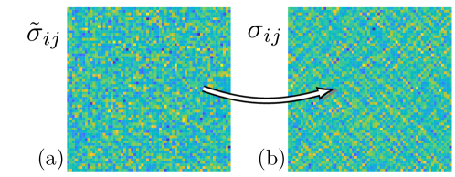
From this state we then instantaneously quench the temperature to 0, so that the velocity field vanishes. Since the state is not in mechanical equilibrium, it will relax under the action of the quench stress σ~ij\tilde{\sigma}_{ij} until it finds a state of mechanical equilibrium, as depicted in Figure 1. The process ends as soon as a state of mechanical equilibrium is found. We will then compute the disorder-averaged Green’s function of the IS.

Since our aim is to model the emergence of structure in the glass, we wish to consider the simplest possible model of the dense liquid. Only the short-time response of the liquid is relevant, so we consider the latter as an initial homogeneous elastic continuum with elastic constants λ~\tilde{\lambda} and μ~\tilde{\mu}, which gives the elastic modulus tensor Cijkl=λ~δijδkl+μ~(δikδjl+δilδjk)C_{ijkl}=\tilde{\lambda}\delta_{ij}\delta_{kl}+\tilde{\mu}(\delta_{ik}\delta_{jl}+\delta_{il}\delta_{jk}). We assume, for simplicity, that these constants are spatially uniform. When the temperature is removed, the continuum deforms under the quench stress, just as a crumpled elastic membrane will relax when external constraints are removed. For simplicity we ignore inertia during the quench, so our model is one of an overdamped quench. This is equivalent to gradient descent as performed in numerical simulations.

Although crude, this model is perhaps the simplest that captures the final stages of descent into an IS; more advanced models could allow the liquid to have non-trivial structural correlations and consider inertia in the quenching process.

Refer to caption
Figure 1: Illustration of random quench model. From (a) an initial disordered state with quench stress σ~ij\tilde{\sigma}_{ij}, we allow the system to relax to an inherent state with stress σij\sigma_{ij}, (b). Illustrated here are σ~xy\tilde{\sigma}_{xy} and σxy\sigma_{xy} for μ/λ=0.1\mu/\lambda=0.1. The long-range correlations in σxy\sigma_{xy} are apparent.

We aim to describe universal properties of this process. Since we work in the continuum, the relevant distribution of σ~ij(r)\tilde{\sigma}_{ij}(\vec{r}) can be inferred using field-theoretical arguments DeGiuli (2018a, b). Indeed, under our assumption of a featureless liquid, under coarse-graining the quench stress field will retain only short-range correlations. As we eventually seek the small qq behaviour of the solid, we take this small length scale to 0 immediately to obtain a simple Gaussian distribution of the symmetric tensor field σ~ij(r)\tilde{\sigma}_{ij}(\vec{r}):

[σ~]exp(12r[s1~σij~σij+s2σ~iiσ~jj]),\displaystyle\mathbb{P}[\tilde{\sigma}]\propto\exp\left(-\mbox{$\frac{1}{2}$}\int_{r}\left[s_{1}\tilde{}\mathrlap{\!\not{\phantom{\sigma}}}\sigma_{ij}\tilde{}\mathrlap{\!\not{\phantom{\sigma}}}\sigma_{ij}+s_{2}\tilde{\sigma}_{ii}\tilde{\sigma}_{jj}\right]\right), (3)

where ~σij=σ~ij1dδijσ~kk\tilde{}\mathrlap{\!\not{\phantom{\sigma}}}\sigma_{ij}=\tilde{\sigma}_{ij}-\mbox{$\frac{1}{d}$}\delta_{ij}\tilde{\sigma}_{kk} is the deviatoric stress, and s1s_{1} and s2s_{2} are parameters related to the magnitude of quench stress by

~σij(r)~σij(0)¯\displaystyle\overline{\tilde{}\mathrlap{\!\not{\phantom{\sigma}}}\sigma_{ij}(\vec{r})\tilde{}\mathrlap{\!\not{\phantom{\sigma}}}\sigma_{ij}(0)} =d21s1δ(r),\displaystyle=\frac{d^{2}-1}{s_{1}}\delta(\vec{r}), (4)
σ~ii(r)σ~jj(0)¯\displaystyle\overline{\tilde{\sigma}_{ii}(\vec{r})\tilde{\sigma}_{jj}(0)} =1s2δ(r)\displaystyle=\frac{1}{s_{2}}\delta(\vec{r}) (5)

in dd dimensions. The constant component of the quench stress will be treated separately.

Standard renormalization arguments DeGiuli (2018a, b) predict that corrections to (3) will introduce a length scale aa which is on the order of the relevant microscopic length, namely the particle radius. We therefore expect our model to be valid on scales much larger than this size. In particular, the Gaussian distribution (3) should be valid, so long as the liquid state does not have relevant long-range correlations. In our continuum treatment, we will employ a cutoff Λ2π/a\Lambda\approx 2\pi/a in momentum space, so that corrections to (3) need not be explicitly incorporated.

Consider the displacement field ui(r)u_{i}(\vec{r}) along the quench. At any moment, there is an instantaneous stress field σij[u](r)\sigma_{ij}[\vec{u}](\vec{r}). In an overdamped quench, a new IS will be found as soon as σij\sigma_{ij} is in mechanical equilibrium. (If inertia were considered, the system could jump over shallow minima before finding a resting state.) Di Donna and Lubensky found the new IS stress σij(r)\sigma_{ij}(\vec{r}) and the elastic modulus tensor Cijkl(r)=Cijkl+δCijkl(r)C^{\prime}_{ijkl}(\vec{r})=C_{ijkl}+\delta C_{ijkl}(\vec{r}) around the IS, to leading order in uiu_{i}, for arbitrary quench stress fields σ~ij(r)\tilde{\sigma}_{ij}(\vec{r}) with zero spatial average. The result is a pair of linear functionals

δCijkl(q)\displaystyle\delta C_{ijkl}(\vec{q}) =𝒮ijklmn(q)σ~mn(q)\displaystyle=\mathscr{S}_{ijklmn}(\vec{q})\tilde{\sigma}_{mn}(\vec{q}) (6)
σij(q)\displaystyle\sigma_{ij}(\vec{q}) =𝒫ijkl(q)σ~kl(q)\displaystyle=\mathscr{P}_{ijkl}(\vec{q})\tilde{\sigma}_{kl}(\vec{q}) (7)

in Fourier space, where 𝒮\mathscr{S} and 𝒫\mathscr{P} depend on the elastic moduli and the momentum q\vec{q}. Explicitly, these take the form

𝒮ijklmn(q)\displaystyle\mathscr{S}_{ijklmn}(\vec{q}) =12(1c)[2c(δijδkeδlf+δklδieδjf)+(1c)(δikδjeδlf+δjlδieδkf+δilδjeδkf+δjkδieδlf)]Vefmn\displaystyle=-\frac{1}{2(1-c)}[2c(\delta_{ij}\delta_{ke}\delta_{lf}+\delta_{kl}\delta_{ie}\delta_{jf})+(1-c)(\delta_{ik}\delta_{je}\delta_{lf}+\delta_{jl}\delta_{ie}\delta_{kf}+\delta_{il}\delta_{je}\delta_{kf}+\delta_{jk}\delta_{ie}\delta_{lf})]V_{efmn} (8)
𝒫ijkl(q)\displaystyle\mathscr{P}_{ijkl}(\vec{q}) =12PTikPTjl+12PTilPTjk11+2μPTijq^kq^l,\displaystyle=\frac{1}{2}{P^{T}}_{ik}{P^{T}}_{jl}+\frac{1}{2}{P^{T}}_{il}{P^{T}}_{jk}-\frac{1}{1+2\mu}{P^{T}}_{ij}\hat{q}_{k}\hat{q}_{l}, (9)

where c=1/(1+2μ)c=1/(1+2\mu), PTij=δijq^iq^j{P^{T}}_{ij}=\delta_{ij}-\hat{q}_{i}\hat{q}_{j}, and

Vefmn=q^e(δfmq^n+δfnq^m)+q^f(δemq^n+δenq^m)2(1+c)q^eq^fq^mq^n.\displaystyle V_{efmn}=\hat{q}_{e}(\delta_{fm}\hat{q}_{n}+\delta_{fn}\hat{q}_{m})+\hat{q}_{f}(\delta_{em}\hat{q}_{n}+\delta_{en}\hat{q}_{m})-2(1+c)\hat{q}_{e}\hat{q}_{f}\hat{q}_{m}\hat{q}_{n}. (10)

Ref. DiDonna and Lubensky (2005) did not include any constant component of the quench stress, but this is easily added. To leading order in uu, we find that if σ~ij(r)¯=p¯δij\overline{\tilde{\sigma}_{ij}(\vec{r})}={\overline{p}}\delta_{ij}, then this is equivalent to replacing the Lamé moduli by λ=λ~dp¯\lambda=\tilde{\lambda}-d{\overline{p}} and μ=μ~+p¯\mu=\tilde{\mu}+{\overline{p}}.

II.1 Stress correlations & elastic moduli fluctuations:

Combining Eqs.(6),(7) with (3) immediately yields predictions for the distribution of local elastic moduli and the distribution of IS stress.

The derivation of the IS stress distribution is nontrivial because of mechanical equilibrium, which is satisfied by σ\sigma but not by σ~\tilde{\sigma}. The derivation is sketched in Appendix 1.

The result is conveniently represented in terms of a gauge field Henkes and Chakraborty (2009); DeGiuli (2018a, b). In d=2d=2 we can write σij=ϵikϵjlklψ\sigma_{ij}=\epsilon_{ik}\epsilon_{jl}\partial_{k}\partial_{l}\psi, where ϵ\epsilon is the antisymmetric tensor with ϵ12=ϵ21=1\epsilon_{12}=-\epsilon_{21}=1 and ϵ11=ϵ22=0\epsilon_{11}=\epsilon_{22}=0, and we predict

[σ[ψ]]exp(12η~rtr2σ),d=2,\displaystyle\mathbb{P}[\sigma[\psi]]\propto\exp\left(-\mbox{$\frac{1}{2}$}\tilde{\eta}\int_{r}\mbox{tr}^{2}\sigma\right),\quad d=2, (11)

with

η~=(1+2μ)2s1s24(1+μ)2s2+2μ2s1,d=2.\displaystyle\tilde{\eta}=\frac{(1+2\mu)^{2}s_{1}s_{2}}{4(1+\mu)^{2}s_{2}+2\mu^{2}s_{1}},\quad d=2. (12)

Similarly, in d=3d=3 we can write σij=ϵiklϵjmnkmΨln\sigma_{ij}=\epsilon_{ikl}\epsilon_{jmn}\partial_{k}\partial_{m}\Psi_{ln} and we predict

[σ[Ψ]]exp(12r[ηtr2(σ)+gtrσ2]),d=3,\displaystyle\mathbb{P}[\sigma[\Psi]]\propto\exp\left(-\mbox{$\frac{1}{2}$}\int_{r}\left[\eta\;\mbox{tr}^{2}(\sigma)+g\;\mbox{tr}\sigma^{2}\right]\right),\quad d=3, (13)

where

η\displaystyle\eta =s124μ2s1+(912μ2)s28μ2s1+3(3+2μ)2s2d=3\displaystyle=-\frac{s_{1}}{2}\frac{4\mu^{2}s_{1}+(9-12\mu^{2})s_{2}}{8\mu^{2}s_{1}+3(3+2\mu)^{2}s_{2}}\quad d=3 (14)
g\displaystyle g =s12.\displaystyle=\frac{s_{1}}{2}. (15)

Eq.(11) and Eq.(13) are in precise agreement with DeGiuli (2018a, b) when boundary effects are neglected. We emphasize that σ\sigma is a functional of ψ\psi in d=2d=2 and Ψ\Psi in d=3d=3 and thus these distributions are nontrivial. As shown in Appendix 1, these gauge fields are necessary to enforce the constraints on the stress tensor σT=σ\sigma^{T}=\sigma and σ=0\nabla\cdot\sigma=0. They predict anisotropic long-range correlations in the stress field, as discussed at length in DeGiuli (2018a, b).

We can also determine the distribution of local elastic moduli. We focus here on the bulk modulus fluctuation δK=δCiikk/d2\delta K=\delta C_{iikk}/d^{2} and shear modulus fluctuation δμ=[dδCijijδCiijj]/(d3+d22d)\delta\mu=[d\delta C_{ijij}-\delta C_{iijj}]/(d^{3}+d^{2}-2d). These are predicted to be Gaussian, with fluctuations

δK(r)δK(0)\displaystyle\langle\delta K(\vec{r})\delta K(0)\rangle =2s1d4[¯d+(5c¯d+4)2+s1ds2d2s2(d+1+5c¯d)2]δ(r)\displaystyle=\frac{2}{s_{1}d^{4}}\left[\mathchar 22\relax\mkern-9.0mud+(5c\mathchar 22\relax\mkern-9.0mud+4)^{2}+\frac{s_{1}-ds_{2}}{d^{2}s_{2}}(d+1+5c\mathchar 22\relax\mkern-9.0mud)^{2}\right]\delta(\vec{r}) (16)
δμ(r)δμ(0)\displaystyle\langle\delta\mu(\vec{r})\delta\mu(0)\rangle =2s1d2(d+2)2¯d[(d2+1)2+¯d(2d+4+c(d22d5))2\displaystyle=\frac{2}{s_{1}d^{2}(d+2)^{2}\mathchar 22\relax\mkern-9.0mud}\left[(d^{2}+1)^{2}+\mathchar 22\relax\mkern-9.0mud(2d+4+c(d^{2}-2d-5))^{2}\right. (17)
+¯d(d22d+5+c(d22d5))2s1ds2d2s2]δ(r)\displaystyle\quad\left.+\mathchar 22\relax\mkern-9.0mud(d^{2}-2d+5+c(d^{2}-2d-5))^{2}\frac{s_{1}-ds_{2}}{d^{2}s_{2}}\right]\delta(\vec{r})

with ¯d=d1\mathchar 22\relax\mkern-9.0mud=d-1 and c=1/(1+2μ)c=1/(1+2\mu). The strictly local nature of these correlations is a consequence of the local quench stress correlations. We expect corrections to these correlations only at the particle scale, as observed in generic models Mizuno et al. (2016); Shakerpoor et al. (2020).

Eqs. (12), (14), (15), (16), and (17) can be used to relate the strength of stress correlations and elastic moduli fluctuations to the quench stress, and to each other.

II.2 Green’s function & effective medium theory:

We now proceed to determine the Green’s function G¯ij\overline{G}_{ij}. We consider response at frequency ω\omega and write the elasto-dynamic equation as a tensorial linear operator A^(ω;σ)\hat{A}(\omega;\sigma) acting on u\vec{u},

Ail(ω)ρω2δil(jSijkl)kSijkljk\displaystyle A_{il}(\omega)\equiv-\rho\omega^{2}\delta_{il}-(\partial_{j}S_{ijkl})\partial_{k}-S_{ijkl}\partial_{j}\partial_{k}

We need to compute the Green’s function G^(r;r0)\hat{G}(\vec{r};\vec{r}_{0}), the solution to

A^(ω)u=F0δ(r),\displaystyle\hat{A}(\omega)\cdot\vec{u}=\vec{F}_{0}\delta(\vec{r}),

This is a challenging task because G^\hat{G} depends on the specific realization of the quenched stress field, which plays the role of disorder. We would be content to compute G^¯\overline{\hat{G}}, the disorder-averaged Green’s function. In our model, this cannot be done exactly. We employ the effective medium theory (EMT), a mean-field approximation that determines the optimal complex elastic moduli μE(ω)\mu_{E}(\omega) and λE(ω)\lambda_{E}(\omega) to represent the effect of scattering by disorder.

This task is similar to that faced in strongly interacting quantum systems, where one would like to compute the Green’s function averaged over quantum fluctuations Köhler et al. (2013). In that context, effective medium techniques have been developed under the name dynamical mean-field theory Georges et al. (1996), which was shown to be exact in the limit of infinite dimensions, the mean-field limit Metzner and Vollhardt (1989).

We derive a self-consistent equation for the effective elastic modulus tensor SijklE(ω)S_{ijkl}^{E}(\omega) under the effective medium approximation. We decompose the full elastic moduli into the effective moduli and the remainder ΔSijklSijklSijklE(ω)\Delta S_{ijkl}\equiv S_{ijkl}-S^{E}_{ijkl}(\omega). The key step is to choose SijklE(ω)S_{ijkl}^{E}(\omega) such that the disorder-average of the true Green’s function equals the EMT Green’s function:

Gij(r;r0)¯=GijE(rr0),\displaystyle\overline{\;G_{ij}(\vec{r};\vec{r}_{0})\;}=G^{E}_{ij}(\vec{r}-\vec{r}_{0}), (18)

where GijE(rr0)G^{E}_{ij}(\vec{r}-\vec{r}_{0}) is the Green’s function in terms of SijklE(ω)S_{ijkl}^{E}(\omega). Here we assume that homogeneity and isotropy are restored in the effective Green’s function, thus

GijE(r)=α=T,LqGα(q,ω)Pijαeiqr,\displaystyle G^{E}_{ij}(\vec{r})=\sum_{\alpha=T,L}\int_{q}G_{\alpha}(q,\omega)\;P_{ij}^{\alpha}\;e^{i\vec{q}\cdot\vec{r}}, (19)

where GT(q,ω)=1/(ρω2+μE(ω)q2),GL(q,ω)=1/(ρω2+λE(ω)q2)G_{T}(q,\omega)=1/(-\rho\omega^{2}+\mu_{E}(\omega)q^{2}),G_{L}(q,\omega)=1/(-\rho\omega^{2}+\lambda_{E}(\omega)q^{2}), PijT=δijq^iq^j,PijL=q^iq^jP_{ij}^{T}=\delta_{ij}-\hat{q}_{i}\hat{q}_{j},P_{ij}^{L}=\hat{q}_{i}\hat{q}_{j}, and q=ddq/(2π)d\int_{q}=\int d^{d}q/(2\pi)^{d} over the region q<Λq<\Lambda. ( T and L stand for transverse and longitudinal, respectively. )

Let us note that the equation (18) cannot be imposed exactly, except in very simple models. One example of the latter is when a lattice has only a single bond with heterogeneity DeGiuli et al. (2014a). EMT is therefore a small-disorder (mean-field) approximation.

The EMT introduces one parameter, vv, the correlation volume over which the EMT G¯ij\overline{G}_{ij} is attained; we take v=1/q1v=1/\int_{q}1 which is derived from comparison with previous results on spring networks DeGiuli et al. (2014a). This corresponds to a correlation volume on the order of the particle size.

The derivation of the EMT within the field theory formalism is sketched in Appendix 3.

We find that the final disorder-averaged Green’s function depends on a random d×dd\times d matrix in the Gaussian orthogonal ensemble (GOE) Mehta (2004). Here we report results for the limit μ1\mu\ll 1, for which λE=1+𝒪(μ)\lambda_{E}=1+\mathscr{O}(\mu): to leading order, the longitudinal Lamé modulus is not modified by the quench. Physically this limit means that the system is fragile like molecular glasses and weakly jammed materials, but it is adopted only for simplicity here. In this regime the key control parameter is

e=(v(d+2)3s1μ4/4)1,\displaystyle e=\big{(}v(d+2)^{3}s_{1}\mu^{4}/4\big{)}^{-1}, (20)

which measures the strength of moduli fluctuations. Introducing a fluctuating shear modulus μr(x)=μ+e1/2μx¯d/d\mu_{r}(x)=\mu+e^{1/2}\mu x\mathchar 22\relax\mkern-9.0mud/d we find that μE\mu_{E} satisfies

0=𝑑xκ(x)(μEμr(x))1(1μr(x)μE)¯dd(1+ρω2vqGT(q,ω)),\displaystyle 0=\int dx\frac{\kappa(x)(\mu_{E}-\mu_{r}(x))}{1-(1-\mbox{$\frac{\mu_{r}(x)}{\mu_{E}}$})\mbox{$\frac{\mathchar 22\relax\mkern-9.0mud}{d}$}\left(1+\rho\omega^{2}v\int_{q}G_{T}(q,\omega)\right)}, (21)

where κ(x)\kappa(x) is the convolution of a Gaussian with the spectral density of the GOE matrix. Note that the random variable xx can be interpreted as a normalized space-dependent shear modulus as discussed in Appendix 3. We emphasize that the GOE matrix whose spectrum appears in (21) is not put into the model, but emerges from its solution.

Remarkably, Eq.(21) exactly matches the form of an equation derived in DeGiuli et al. (2014a), under the identifications μEk\mu_{E}\to k_{\parallel}, an effective longitudinal stiffness; μrkα\mu_{r}\to k_{\alpha}, a fluctuating stiffness; and z0=2d2/¯dz_{0}=2d^{2}/\mathchar 22\relax\mkern-9.0mud, a lattice parameter. In DeGiuli et al. (2014a), and in companion works DeGiuli et al. (2014b, 2015), the stiffnesses kαk_{\alpha} were microscopic spring constants, whose distribution (kα)\mathbb{P}(k_{\alpha}) was assumed to take simple tractable forms. In contrast, here we derive the relevant distribution κ(x)\kappa(x) from our model of quench dynamics.

II.3 Wigner semicircle:

The simplest limit is dd\to\infty, for which we expect EMT to be exact Georges et al. (1996). In d=d=\infty the GOE spectrum is given by the Wigner semicircle law ρW(x)=2dx2/(πd)\rho_{W}(x)=\sqrt{2d-x^{2}}/(\pi d) and κ(x)=ρ(x)\kappa(x)=\rho(x) up to irrelevant corrections of relative order 1/d21/d^{2}. Using the fact that ρW\rho_{W} is supported on a finite interval (2d,2d)(-\sqrt{2d},\sqrt{2d}), we can determine the relevant scaling e1/de\sim 1/d and x1x\sim 1 for large dd. Defining ω~=ωAd/μ\tilde{\omega}=\omega\sqrt{A_{d}/\mu} with Ad=vρqq2A_{d}=v\rho\int_{q}q^{-2}, we take ω~1\tilde{\omega}\sim 1. Then we can derive a cubic equation for y=μE/μy=\mu_{E}/\mu:

0=y3y2+d2e[y+Adμω2],\displaystyle 0=y^{3}-y^{2}+\mbox{$\frac{d}{2}$}e\left[y+\mbox{$\frac{A_{d}}{\mu}$}\omega^{2}\right], (22)

The same equation has recently been derived for a lattice EMT, and analyzed in detail Shimada et al. (2020b). Translating these results, we find: (i) the solid is stable for e<ec=1/(2d)e<e_{c}=1/(2d); (ii) near ece_{c} and at small ω\omega, xx satisfies a quadratic equation equivalent to that derived in DeGiuli et al. (2014a), giving

μE(ω)=12μiμAd2(ω2ω02),\displaystyle\mu_{E}(\omega)=\mbox{$\frac{1}{2}$}\mu-i\sqrt{\mbox{$\frac{\mu A_{d}}{2}$}(\omega^{2}-\omega_{0}^{2})}, (23)

where the onset frequency is

ω0=μdAd(ece)\displaystyle\omega_{0}=\sqrt{\mbox{$\frac{\mu d}{A_{d}}$}(e_{c}-e)} (24)

In this limit the vibrational properties are thus equivalent to those discussed in DeGiuli et al. (2014a). In particular, the density of vibrational states is g(ω)=(2ω/π)ImG¯ii(0)(2¯dω/π)Im[μE]qq2/|μE|2g(\omega)=(2\omega/\pi)\mbox{Im}\overline{G}_{ii}(0)\approx-(2\mathchar 22\relax\mkern-9.0mud\omega/\pi)\mbox{Im}[\mu_{E}]\int_{q}q^{-2}/|\mu_{E}|^{2}, from which it follows that for ω>ω0\omega>\omega_{0} Eq.(23) gives the non-Debye law g(ω)ω2g(\omega)\propto\omega^{2} discussed in the introduction.

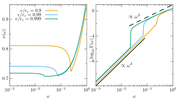
Scattering experiments measure the dynamic structure factor, from which one can extract, at each frequency ω\omega, a sound speed ν(ω)=|μE|/Re[μE1/2]\nu(\omega)=|\mu_{E}|/\mbox{Re}[\mu_{E}^{1/2}] DeGiuli et al. (2014a) and the sound attentuation Γ(ω)ωIm[μE]/Re[μE]\Gamma(\omega)\approx-\omega\mbox{Im}[\mu_{E}]/\mbox{Re}[\mu_{E}] DeGiuli et al. (2014a). In experiments Baldi et al. (2010, 2011b) and simulations Mizuno and Ikeda (2018) the sound speed is non-monotonic in frequency, showing a dip in the boson peak range where the sound attentuation crosses over from ωd+1\omega^{d+1} to ω2\omega^{2} behaviour; these features are reproduced by Eqs.(22),(23). Representative plots for these quantities in d=3d=3 are shown in Fig.3.

Quantitatively, we find Γ(ω)(πdμe/4)vρω2g(ω)/Re[μE]\Gamma(\omega)\approx(\pi d\mu e/4)v\rho\omega^{2}g(\omega)/\mbox{Re}[\mu_{E}]. In deriving Eq.(22), we ignored the hydrodynamic pole in the Green’s function, which leads to the Debye law g(ω)ωd1g(\omega)\sim\omega^{d-1} for ω<ω0\omega<\omega_{0}. This thus leads to Γ(ω)ωd+1\Gamma(\omega)\sim\omega^{d+1}, which is Rayleigh scattering. Its amplitude is proportional to the variance of elastic moduli fluctuations, as observed Kapteijns et al. (2020).

Refer to caption
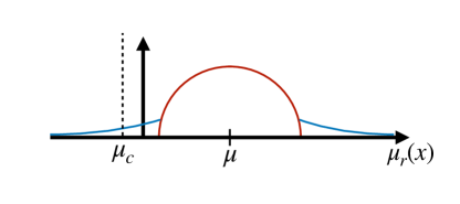
Figure 2: Schematic distribution of fluctuating shear modulus μr\mu_{r}. In d=d=\infty, the distribution is a semi-circle; in finite dimensions, this develops a tail, which can lead to instability in large systems.

II.4 Finite-dimensional corrections:

GOE matrices have a spectrum whose bulk resembles the Wigner semicircle in all dimensions, with oscillatory corrections. Eq.(22) and its consequences can then be used in any dimension dd to determine the leading physics. However, for d<d<\infty, there is a new phenomenon completely absent in the Wigner semicircle: the spectrum develops an exponentially-decaying tail, as shown in Figure 2. This tail, which is Gaussian in d=2d=2 and d=3d=3, adds new excitations, which we expect to be localized. Formally, the tail extends to ±\pm\infty, implying that there are now unstable modes. Indeed, from Eq.(21), one can determine a stability condition μr>μc=Re[μE]/¯d\mu_{r}>\mu_{c}=-\mbox{Re}[\mu_{E}]/\mathchar 22\relax\mkern-9.0mud Shimada et al. (2020b); the smallest modulus can be negative, but small, scaling as 1/d1/d. However, our results are derived for systems in the thermodynamic limit. Since xx corresponds to a spatially fluctuating modulus, in a system of NN particles there are approximately NN values of xx sampled from κ(x)\kappa(x). Define xx^{*} from 1/N=x𝑑xκ(x)1/N=\int_{-\infty}^{x^{*}}dx\;\kappa(x). When μr(x)>μc\mu_{r}(x^{*})>\mu_{c}, corresponding to small systems, the tail is irrelevant and the system is stable. In this case, using Allez et al. (2012), we find that μE\mu_{E} has a contribution δμiω2\delta\mu\sim-i\omega^{2} in the regime 0<ω<ω00<\omega<\omega_{0}, which will lead to g(ω)ω3g(\omega)\sim\omega^{3}, on top of the Debye contribution. Instead, when μr(x)<μc\mu_{r}(x^{*})<\mu_{c}, our quench has ended in an unstable state, and must further relax to a true inherent state. If κ(x)\kappa(x) is modified ad-hoc to vanish at μr(xc)=μc\mu_{r}(x_{c})=\mu_{c} as κ(x)(xxc)β\kappa(x)\sim(x-x_{c})^{\beta}, then instead we find that g(ω)ω2β+1g(\omega)\sim\omega^{2\beta+1} Shimada et al. (2020b).

These results are in qualitative agreement with previous findings, which indeed found a density of localized modes g(ω)ωαg(\omega)\sim\omega^{\alpha} with α<4\alpha<4 in small systems Lerner (2020). In our model, the global stability of the system is controlled by the parameter ee. However, we do not enforce local stability of the final state. Since α=4\alpha=4 is typically observed, these results imply that our assumption of an overdamped quench cannot be realistic in large systems. Future work should explicitly incorporate a condition of local mechanical stability in the IS, to properly predict the form of κ(x)\kappa(x) in realistic systems.

III Conclusion:

We propose a model for universal properties of amorphous solids based on the quench into an inherent state. Under a single universal distribution of quench stress, our model predicts (i) short-range correlations of elastic moduli, as observed Mizuno et al. (2016); Kapteijns et al. (2020); Shakerpoor et al. (2020); (ii) long-range correlations of the IS stress, as observed Lemaître (2015, 2017); Mizuno and Mossa (2019); (iii) exact reduction to previous models, shown to reproduce universal vibrational anomalies DeGiuli et al. (2014a); Shimada et al. (2020b); and (iv) a tail of potentially unstable modes, beyond mean-field predictions, which leads to g(ω)ω3g(\omega)\sim\omega^{3} in small systems and can rationalize larger exponents g(ω)ωαg(\omega)\sim\omega^{\alpha} in large, stable systems.

Refer to caption
Figure 3: (a) Sound speed ν(ω)\nu(\omega) and (b) sound attenuation Γ(ω)\Gamma(\omega) for indicated values of e/ece/e_{c}, in d=3d=3.

New results include the relationship between the elastic-moduli fluctuations and the stress correlations; explicit expressions for the stress correlations in arbitrary dimension; justification of mean-field models which formerly were derived from lattice models; and the inevitable extension of mean-field models to have an eigenvalue tail in finite dimensions.

Our model is based on an overdamped quench, which enforces mechanical equilibrium in the IS, but does not enforce stability. This allows unstable configurations, like a pencil standing on its head. At the global level, stability is ensured by choosing parameters such that all vibrational modes have a positive real frequency; in particular we should have e<ece<e_{c} as described above. However, we do not enforce stability at each point in space. In particular, the Hessian field Hij(r,r)=2E/(ui(r)uj(r))H_{ij}(\vec{r},\vec{r}^{\prime})=\partial^{2}E/(\partial u_{i}(\vec{r})\partial u_{j}(\vec{r}^{\prime})) that controls local stability could have regions where it is not positive-definite. We predict Gaussian fluctuations of local elastic moduli, as observed in Mizuno et al. (2016); Shakerpoor et al. (2020), while it has very recently been argued that the moduli have a power-law tail due to localized modes Kapteijns et al. (2020). We expect that these modes are created by local relaxation in regions of an unstable Hessian. To rigorously predict the density of small-frequency localized modes in large systems, and their potential modifications to elastic moduli fluctuations, future work should thus add local stability as a remaining feature to the model.

In addition, we have assumed for simplicity that the initial pre-quenched liquid state has homogenous short-time elastic constants. It would be useful and relevant to allow these to have short-range Gaussian fluctuations, which will be transformed under the quench and may alter the elastic properties of the glass.

Acknowledgments: We are grateful to E. Lerner and M. Wyart for comments on the manuscript, and to the referees for useful comments. MS thanks H. Mizuno for useful information on simulations and A. Ikeda for his encouragement. MS is supported by JSPS KAKENHI Grant No. 19J20036.

References

  • Anderson (1981) A. Anderson, Amorphous Solids: Low Temperature Properties, edited by W. A. Phillips, Topics in Current Physics, Vol. 24 (Springer, Berlin, 1981).
  • Anderson et al. (1972) P. W. Anderson, B. I. Halperin,  and C. M. Varma, Philos. Mag. 25, 1 (1972).
  • Lerner et al. (2016) E. Lerner, G. Düring,  and E. Bouchbinder, Physical Review Letters 117, 035501 (2016).
  • Kapteijns et al. (2018) G. Kapteijns, E. Bouchbinder,  and E. Lerner, Physical review letters 121, 055501 (2018).
  • Lerner and Bouchbinder (2018) E. Lerner and E. Bouchbinder, Physical Review E 97, 032140 (2018).
  • Angelani et al. (2018) L. Angelani, M. Paoluzzi, G. Parisi,  and G. Ruocco, Proceedings of the National Academy of Sciences 115, 8700 (2018).
  • Wang et al. (2019) L. Wang, A. Ninarello, P. Guan, L. Berthier, G. Szamel,  and E. Flenner, Nature communications 10, 1 (2019).
  • Ji et al. (2019) W. Ji, M. Popović, T. W. de Geus, E. Lerner,  and M. Wyart, Physical Review E 99, 023003 (2019).
  • Khomenko et al. (2020) D. Khomenko, C. Scalliet, L. Berthier, D. R. Reichman,  and F. Zamponi, Physical Review Letters 124, 225901 (2020).
  • Buchenau et al. (1992) U. Buchenau, Y. M. Galperin, V. Gurevich, D. Parshin, M. Ramos,  and H. Schober, Physical Review B 46, 2798 (1992).
  • Parshin et al. (2007) D. Parshin, H. Schober,  and V. Gurevich, Physical Review B 76, 064206 (2007).
  • Schirmacher (2006) W. Schirmacher, EPL 73, 892 (2006).
  • Schirmacher et al. (2007) W. Schirmacher, G. Ruocco,  and T. Scopigno, Phys. Rev. Lett. 98, 025501 (2007).
  • Wyart et al. (2005a) M. Wyart, S. Nagel,  and T. Witten, EPL (Europhysics Letters) 72, 486 (2005a).
  • Wyart et al. (2005b) M. Wyart, L. E. Silbert, S. R. Nagel,  and T. A. Witten, Physical Review E 72, 051306 (2005b).
  • DeGiuli et al. (2014a) E. DeGiuli, A. Laversanne-Finot, G. A. Düring, E. Lerner,  and M. Wyart, Soft Matter 10, 5628 (2014a).
  • Mizuno and Ikeda (2018) H. Mizuno and A. Ikeda, Physical Review E 98, 062612 (2018).
  • Shimada et al. (2018) M. Shimada, H. Mizuno,  and A. Ikeda, Physical Review E 97, 022609 (2018).
  • Shimada et al. (2020a) M. Shimada, H. Mizuno, L. Berthier,  and A. Ikeda, Physical Review E 101, 052906 (2020a).
  • Lerner and Bouchbinder (2017) E. Lerner and E. Bouchbinder, Physical Review E 96, 020104 (2017).
  • Paoluzzi et al. (2019) M. Paoluzzi, L. Angelani, G. Parisi,  and G. Ruocco, Physical review letters 123, 155502 (2019).
  • Lerner (2020) E. Lerner, Physical Review E 101, 032120 (2020).
  • Rufflé et al. (2006) B. Rufflé, G. Guimbretiere, E. Courtens, R. Vacher,  and G. Monaco, Physical review letters 96, 045502 (2006).
  • Monaco and Giordano (2009) G. Monaco and V. M. Giordano, Proceedings of the national Academy of Sciences 106, 3659 (2009).
  • Baldi et al. (2011a) G. Baldi, V. M. Giordano,  and G. Monaco, Physical Review B 83, 174203 (2011a).
  • Ruta et al. (2012) B. Ruta, G. Baldi, F. Scarponi, D. Fioretto, V. Giordano,  and G. Monaco, The Journal of chemical physics 137, 214502 (2012).
  • Mizuno et al. (2016) H. Mizuno, L. E. Silbert,  and M. Sperl, Physical review letters 116, 068302 (2016).
  • Mizuno and Mossa (2019) H. Mizuno and S. Mossa, Condensed Matter Physics 22 (2019).
  • Shakerpoor et al. (2020) A. Shakerpoor, E. Flenner,  and G. Szamel, Soft Matter 16, 914 (2020).
  • Kapteijns et al. (2020) G. Kapteijns, D. Richard, E. Bouchbinder,  and E. Lerner,   (2020), arXiv:2008.08337 [cond-mat.soft] .
  • Lemaître (2015) A. Lemaître, The Journal of chemical physics 143, 164515 (2015).
  • Lemaître (2017) A. Lemaître, Physical Review E 96, 052101 (2017).
  • Note (1) These are inferred from strain measurements in colloidal glassesChikkadi et al. (2011); Jensen et al. (2014); Illing et al. (2016) and granular media Le Bouil et al. (2014).
  • Wang et al. (2020) Y. Wang, Y. Wang,  and J. Zhang, arXiv preprint arXiv:2004.06357  (2020).
  • DiDonna and Lubensky (2005) B. DiDonna and T. Lubensky, Physical Review E 72, 066619 (2005).
  • Morante et al. (2006) S. Morante, G. Rossi,  and M. Testa, The Journal of chemical physics 125, 034101 (2006).
  • DeGiuli (2018a) E. DeGiuli, Phys. Rev. E 98, 033001 (2018a).
  • DeGiuli (2018b) E. DeGiuli, Physical review letters 121, 118001 (2018b).
  • Henkes and Chakraborty (2009) S. Henkes and B. Chakraborty, Phys. Rev. E 79, 061301 (2009).
  • Köhler et al. (2013) S. Köhler, G. Ruocco,  and W. Schirmacher, Physical Review B 88, 064203 (2013).
  • Georges et al. (1996) A. Georges, G. Kotliar, W. Krauth,  and M. J. Rozenberg, Reviews of Modern Physics 68, 13 (1996).
  • Metzner and Vollhardt (1989) W. Metzner and D. Vollhardt, Physical review letters 62, 324 (1989).
  • Mehta (2004) M. L. Mehta, Random matrices (Elsevier, 2004).
  • DeGiuli et al. (2014b) E. DeGiuli, E. Lerner, C. Brito,  and M. Wyart, Proceedings of the National Academy of Sciences 111, 17054 (2014b).
  • DeGiuli et al. (2015) E. DeGiuli, E. Lerner,  and M. Wyart, The Journal of chemical physics 142, 164503 (2015).
  • Shimada et al. (2020b) M. Shimada, H. Mizuno,  and A. Ikeda, Soft Matter  (2020b).
  • Baldi et al. (2010) G. Baldi, V. Giordano, G. Monaco,  and B. Ruta, Physical Review Letters 104, 195501 (2010).
  • Baldi et al. (2011b) G. Baldi, V. Giordano, G. Monaco,  and B. Ruta, Journal of Non-Crystalline Solids 357, 538 (2011b).
  • Allez et al. (2012) R. Allez, J.-P. Bouchaud,  and A. Guionnet, Physical review letters 109, 094102 (2012).
  • Chikkadi et al. (2011) V. Chikkadi, G. Wegdam, D. Bonn, B. Nienhuis,  and P. Schall, Physical Review Letters 107, 198303 (2011).
  • Jensen et al. (2014) K. Jensen, D. A. Weitz,  and F. Spaepen, Physical Review E 90, 042305 (2014).
  • Illing et al. (2016) B. Illing, S. Fritschi, D. Hajnal, C. Klix, P. Keim,  and M. Fuchs, Physical review letters 117, 208002 (2016).
  • Le Bouil et al. (2014) A. Le Bouil, A. Amon, S. McNamara,  and J. Crassous, Physical review letters 112, 246001 (2014).
  • Kirkpatrick (1973) S. Kirkpatrick, Reviews of modern physics 45, 574 (1973).
  • Düring et al. (2013) G. Düring, E. Lerner,  and M. Wyart, Soft Matter 9, 146 (2013).
  • Zinn-Justin (1996) J. Zinn-Justin, Quantum field theory and critical phenomena (Clarendon Press, 1996).

IV Appendix 1. Derivation of stress correlations:

Here we show how to derive the distribution of the inherent stress field. In particular we show that our model predicts the observed long-range stress correlations, and moreover connects the magnitude of these correlations to the coefficients controlling vibrational properties. We use ¯\overline{\cdot} to denote a disorder average, not to be confused with the Grassmann-conjugation defined elsewhere.

The distribution of σ\sigma is

[σ]\displaystyle\mathbb{P}[\sigma] =ijδ[σij𝒫ijklσ~kl]¯\displaystyle=\overline{\prod_{ij}\delta\left[\sigma_{ij}-\mathscr{P}_{ijkl}\tilde{\sigma}_{kl}\right]}
=𝒟τ^exp{iqτij(q)[σij(q)𝒫ijkl(q)σ~kl(q)]}¯\displaystyle=\int{\mathscr{D}}\hat{\tau}\,\overline{\exp\left\{i\int_{q}\tau_{ij}(q)\left[\sigma_{ij}(q)-\mathscr{P}_{ijkl}(q)\tilde{\sigma}_{kl}(q)\right]\right\}}
=𝒟τ^exp[iqτij(q)σij(q)]exp[iqτij(q)𝒫ijkl(q)σ~kl(q)]¯\displaystyle=\int{\mathscr{D}}\hat{\tau}\exp\left[i\int_{q}\tau_{ij}(q)\sigma_{ij}(q)\right]\overline{\exp\left[-i\int_{q}\tau_{ij}(q)\mathscr{P}_{ijkl}(q)\tilde{\sigma}_{kl}(q)\right]}
=𝒟τ^exp[iqτij(q)σij(q)]exp[qτij(q)𝒫ijkl(q)τkl(q)],\displaystyle=\int{\mathscr{D}}\hat{\tau}\exp\left[i\int_{q}\tau_{ij}(q)\sigma_{ij}(q)\right]\exp\left[-\int_{q}\tau_{ij}(q)\mathscr{P}^{\prime}_{ijkl}(q)\tau_{kl}(-q)\right],

where

𝒫ijkl(q)\displaystyle\mathscr{P}^{\prime}_{ijkl}(q) =b1(2μ1+2μ)2PTijPTkl+b22PTikPTjl+b22PTilPTjk+b2(1+2μ)2PTijPTkl\displaystyle=b_{1}\left(\frac{2\mu}{1+2\mu}\right)^{2}{P^{T}}_{ij}{P^{T}}_{kl}+\frac{b_{2}}{2}{P^{T}}_{ik}{P^{T}}_{jl}+\frac{b_{2}}{2}{P^{T}}_{il}{P^{T}}_{jk}+\frac{b_{2}}{(1+2\mu)^{2}}{P^{T}}_{ij}{P^{T}}_{kl}
b1PTijPTkl+b22(PTikPTjl+PTilPTjk).\displaystyle\equiv b_{1}^{\prime}{P^{T}}_{ij}{P^{T}}_{kl}+\frac{b_{2}}{2}\left({P^{T}}_{ik}{P^{T}}_{jl}+{P^{T}}_{il}{P^{T}}_{jk}\right).

and the inverse tensor Kklmn1=b1δklδmn+b2δkmδlnK^{-1}_{klmn}=b_{1}\delta_{kl}\delta_{mn}+b_{2}\delta_{km}\delta_{ln} is determined by the relation KijklKklmn1=δimδjnK_{ijkl}K^{-1}_{klmn}=\delta_{im}\delta_{jn}. Then we have

b1\displaystyle b_{1} =1ds1s2(s2s1d)\displaystyle=-\frac{1}{ds_{1}s_{2}}\left(s_{2}-\frac{s_{1}}{d}\right)
b2\displaystyle b_{2} =1s1.\displaystyle=\frac{1}{s_{1}}.

Since 𝒫ijkl(q)qi=𝒫ijkl(q)qk=0\mathscr{P}^{\prime}_{ijkl}(q)q_{i}=\mathscr{P}^{\prime}_{ijkl}(q)q_{k}=0, it is useful to perform a tensorial Helmholtz decomposition. We change the variable as τij(q)=iqiϕj(q)iqjϕi(q)+Ψij(q)\tau_{ij}(q)=-iq_{i}\phi_{j}(q)-iq_{j}\phi_{i}(q)+\Psi_{ij}(q), where qiΨij(q)=qjΨij(q)=0q_{i}\Psi_{ij}(q)=q_{j}\Psi_{ij}(q)=0. Thus, we have

[σ]\displaystyle\mathbb{P}[\sigma] =𝒟ϕ𝒟Ψexp{iq[iqiϕj(q)iqjϕi(q)+Ψij(q)]σij(q)qΨij(q)𝒫ijkl(q)Ψkl(q)}\displaystyle=\int{\mathscr{D}}\phi{\mathscr{D}}{\Psi}\exp\left\{i\int_{q}\left[-iq_{i}\phi_{j}(q)-iq_{j}\phi_{i}(q)+\Psi_{ij}(q)\right]\sigma_{ij}(q)-\int_{q}\Psi_{ij}(q)\mathscr{P}^{\prime}_{ijkl}(q)\Psi_{kl}(-q)\right\}
=𝒟ϕ𝒟Ψexp{iriϕj(r)[σij(r)+σji(r)]q[Ψij(q)𝒫ijkl(q)Ψkl(q)iΨij(q)σij(q)]}.\displaystyle=\int{\mathscr{D}}\phi{\mathscr{D}}{\Psi}\exp\left\{i\int_{r}\partial_{i}\phi_{j}(r)\left[\sigma_{ij}(r)+\sigma_{ji}(r)\right]-\int_{q}\left[\Psi_{ij}(q)\mathscr{P}^{\prime}_{ijkl}(q)\Psi_{kl}(-q)-i\Psi_{ij}(q)\sigma_{ij}(q)\right]\right\}.

Decomposing Ψ{\Psi} and σ\sigma as Ψ=(Ψ+ΨT)/2+(ΨΨT)/2=ΨS+ΨA{\Psi}=({\Psi}+{\Psi}^{T})/2+({\Psi}-{\Psi}^{T})/2={\Psi}^{S}+{\Psi}^{A} and σ=σS+σA\sigma=\sigma^{S}+\sigma^{A}, we have

[σ]\displaystyle\mathbb{P}[\sigma] =δ[σij(r)σji(r)]δ[iσij(r)]𝒟ΨSexp{q[ΨijS(q)𝒫ijkl(q)ΨklS(q)iΨijS(q)σij(q)]}\displaystyle=\delta\left[\sigma_{ij}(r)-\sigma_{ji}(r)\right]\delta\left[\partial_{i}\sigma_{ij}(r)\right]\int{\mathscr{D}}{\Psi}^{S}\exp\left\{-\int_{q}\left[\Psi_{ij}^{S}(q)\mathscr{P}^{\prime}_{ijkl}(q)\Psi_{kl}^{S}(-q)-i\Psi^{S}_{ij}(q)\sigma_{ij}(q)\right]\right\}
δ[σij(r)σji(r)]δ[iσij(r)]S[σ].\displaystyle\equiv\delta\left[\sigma_{ij}(r)-\sigma_{ji}(r)\right]\delta\left[\partial_{i}\sigma_{ij}(r)\right]\mathbb{P}^{S}[\sigma].

The δ\delta-functions here are exactly the equations of mechanical equilibrium. The remaining symmetric part S[σ]\mathbb{P}^{S}[\sigma] further simplifies to

S[σ]\displaystyle\mathbb{P}^{S}[\sigma] =𝒟ΨSexp{q[ΨijS(q)(b1δijδkl+b2δikδjl)ΨklS(q)iΨijS(q)σij(q)]},\displaystyle=\int{\mathscr{D}}{\Psi}^{S}\exp\left\{-\int_{q}\left[\Psi_{ij}^{S}(q)\left(b_{1}^{\prime}\delta_{ij}\delta_{kl}+b_{2}\delta_{ik}\delta_{jl}\right)\Psi_{kl}^{S}(-q)-i\Psi^{S}_{ij}(q)\sigma_{ij}(q)\right]\right\},

where we used qiΨijS(q)=0q_{i}\Psi^{S}_{ij}(q)=0.

In d=2d=2, setting ΨijS(q)=ϵikϵjlqkqlψ(q)\Psi^{S}_{ij}(q)=-\epsilon_{ik}\epsilon_{jl}q_{k}q_{l}\psi(q), we have

S[σ]\displaystyle\mathbb{P}^{S}[\sigma] =𝒟ψexp{q[ϵimϵjnϵkpϵlq(b1δijδkl+b2δikδjl)qmqnqpqqψ(q)ψ(q)+iϵikϵjlqkqlσij(q)ψ(q)]}\displaystyle=\int{\mathscr{D}}\psi\exp\left\{-\int_{q}\left[\epsilon_{im}\epsilon_{jn}\epsilon_{kp}\epsilon_{lq}\left(b_{1}^{\prime}\delta_{ij}\delta_{kl}+b_{2}\delta_{ik}\delta_{jl}\right)q_{m}q_{n}q_{p}q_{q}\psi(q)\psi(-q)+i\epsilon_{ik}\epsilon_{jl}q_{k}q_{l}\sigma_{ij}(q)\psi(q)\right]\right\}
=𝒟ψexp{q[(b1+b2)q4ψ(q)ψ(q)+iϵikϵjlqkqlσij(q)ψ(q)]}.\displaystyle=\int{\mathscr{D}}\psi\exp\left\{-\int_{q}\left[(b_{1}^{\prime}+b_{2})q^{4}\psi(q)\psi(-q)+i\epsilon_{ik}\epsilon_{jl}q_{k}q_{l}\sigma_{ij}(q)\psi(q)\right]\right\}.

To match the notation of DeGiuli (2018a, b), we set 1/2η~=b1+b21/2\tilde{\eta}=b_{1}^{\prime}+b_{2}. Thus,

S[σ]\displaystyle\mathbb{P}^{S}[\sigma] =𝒟ψexp{η~12qq4[ψ(q)+iϵikϵjlq^kq^lq2η~σij(q)][ψ(q)+iϵmpϵnqq^pq^qq2η~σmn(q)]\displaystyle=\int{\mathscr{D}}\psi\exp\left\{-\frac{\tilde{\eta}^{-1}}{2}\int_{q}q^{4}\left[\psi(q)+i\epsilon_{ik}\epsilon_{jl}\hat{q}_{k}\hat{q}_{l}q^{-2}\tilde{\eta}\sigma_{ij}(q)\right]\left[\psi(-q)+i\epsilon_{mp}\epsilon_{nq}\hat{q}_{p}\hat{q}_{q}q^{-2}\tilde{\eta}\sigma_{mn}(-q)\right]\right.
η~2qϵikϵjlq^kq^lσij(q)ϵmpϵnqq^pq^qσmn(q)}\displaystyle\qquad\left.-\frac{\tilde{\eta}}{2}\int_{q}\epsilon_{ik}\epsilon_{jl}\hat{q}_{k}\hat{q}_{l}\sigma_{ij}(q)\epsilon_{mp}\epsilon_{nq}\hat{q}_{p}\hat{q}_{q}\sigma_{mn}(-q)\right\}
=1Zσexp[η~2qϵikϵjlq^kq^lσij(q)ϵmpϵnqq^pq^qσmn(q)]\displaystyle=\frac{1}{Z_{\sigma}}\exp\left[-\frac{\tilde{\eta}}{2}\int_{q}\epsilon_{ik}\epsilon_{jl}\hat{q}_{k}\hat{q}_{l}\sigma_{ij}(q)\epsilon_{mp}\epsilon_{nq}\hat{q}_{p}\hat{q}_{q}\sigma_{mn}(-q)\right]
=1Zσexp[η~2rtr2σ(r)],\displaystyle=\frac{1}{Z_{\sigma}}\exp\left[-\frac{\tilde{\eta}}{2}\int_{r}\mbox{tr}^{2}\sigma(r)\right],

where ZσZ_{\sigma} is the normalization constant and we used qiσij(q)=0q_{i}\sigma_{ij}(q)=0. The coefficient η~\tilde{\eta} is given by

η~\displaystyle\tilde{\eta} =(1+2μ)22{4μ2b1+[1+(1+2μ)2]b2}.\displaystyle=\frac{(1+2\mu)^{2}}{2\{4\mu^{2}b_{1}+[1+(1+2\mu)^{2}]b_{2}\}}.

In d=3d=3 the computations are similar. The relevant tensorial Helmholtz decomposition is discussed in DeGiuli (2018a).

V Appendix 2. Derivation of elastic moduli fluctuations:

V.0.1 Bulk modulus

Here, we derive fluctuations in bulk modulus. The fluctuating part of SijklS_{ijkl} reads

δSijkl=(𝒮ijklmn+𝒫ikmnδjl)σ~mn.\displaystyle\delta S_{ijkl}=(\mathscr{S}_{ijklmn}+\mathscr{P}_{ikmn}\delta_{jl})\tilde{\sigma}_{mn}.

When we consider a homogeneous bulk deformation εkl=εδkl/d\varepsilon_{kl}=\varepsilon\delta_{kl}/d, the pressure fluctuation is

δp=1dδSiiklεkl=1d2δSiikkε.\displaystyle\delta p=\frac{1}{d}\delta S_{iikl}\varepsilon_{kl}=\frac{1}{d^{2}}\delta S_{iikk}\varepsilon.

Thus, the bulk modulus fluctuation is

δK\displaystyle\delta K =δp/ε=1d2(𝒮iikkmn+𝒫ikmnδik)σ~mn\displaystyle=\delta p/\varepsilon=\frac{1}{d^{2}}(\mathscr{S}_{iikkmn}+\mathscr{P}_{ikmn}\delta_{ik})\tilde{\sigma}_{mn}
=1d2{[4+5c(d1)]q^mq^n+PTmn}σ~mn𝒦mnσ~mn.\displaystyle=-\frac{1}{d^{2}}\left\{[4+5c(d-1)]\hat{q}_{m}\hat{q}_{n}+{P^{T}}_{mn}\right\}\tilde{\sigma}_{mn}\equiv\mathscr{K}_{mn}\tilde{\sigma}_{mn}.

The probability distribution function of δK\delta K can be written as

[δK]\displaystyle\mathbb{P}[\delta K] =δ[δK𝒦:σ¯^]¯\displaystyle=\overline{\delta[\delta K-{\mathscr{K}}:{\hat{\overline{\sigma}}}]}
=𝒟τexp{iqτ(q)[δK(q)𝒦^(q):σ¯^(q)]}¯\displaystyle=\overline{\int{\mathscr{D}}\tau\exp\left\{i\int_{q}\tau(-q)[\delta K(q)-\hat{\mathscr{K}}(q):{\hat{\overline{\sigma}}}(q)]\right\}}
=𝒟τexp[iqτ(q)δK(q)]exp{2qτ(q)τ(q)𝒦^(q):K1:𝒦^(q)}.\displaystyle=\int{\mathscr{D}}\tau\exp\left[i\int_{q}\tau(-q)\delta K(q)\right]{\exp\left\{-2\int_{q}\tau(q)\tau(-q)\hat{\mathscr{K}}(q):K^{-1}:\hat{\mathscr{K}}(-q)\right\}}.

Using the definition of 𝒦^\hat{\mathscr{K}}, we have

𝒦ij(q)Kijkl1𝒦kl(q)\displaystyle\mathscr{K}_{ij}(q)K^{-1}_{ijkl}\mathscr{K}_{kl}(-q) =1d4{b1[4+(5c+1)(d1)]2+b2[4+5c(d1)]2+b2(d1)}Kμ,d4β.\displaystyle=\frac{1}{d^{4}}\left\{b_{1}[4+(5c+1)(d-1)]^{2}+b_{2}[4+5c(d-1)]^{2}+b_{2}(d-1)\right\}\equiv\frac{K_{\mu,d}}{4\beta}.

Finally, we obtain

[δK]\displaystyle\mathbb{P}[\delta K] =1ZKexp[β2Kμ,drδK(r)2].\displaystyle=\frac{1}{Z_{K}}\exp\left[-\frac{\beta}{2K_{\mu,d}}\int_{r}\delta K(r)^{2}\right].

Thus, the correlation of the bulk modulus is

δK(r)δK(0)\displaystyle\left<\delta K(r)\delta K(0)\right> =12βKμ,dδ(r).\displaystyle=\frac{1}{2\beta}K_{\mu,d}\delta(r).

This is always short range.

V.0.2 Shear modulus

The shear modulus fluctuation is

δμ\displaystyle\delta\mu =1(d+2)(d1)(𝒮ijijmn1d𝒮iikkmn+𝒫iimnδjj1d𝒫ikmnδik)σ~mnmnσ~mn,\displaystyle=\frac{1}{(d+2)(d-1)}\left(\mathscr{S}_{ijijmn}-\frac{1}{d}\mathscr{S}_{iikkmn}+\mathscr{P}_{iimn}\delta_{jj}-\frac{1}{d}\mathscr{P}_{ikmn}\delta_{ik}\right)\tilde{\sigma}_{mn}\equiv\mathscr{M}_{mn}\tilde{\sigma}_{mn}, (25)

where

(d+2)d(d1)mn\displaystyle(d+2)d(d-1)\mathscr{M}_{mn} =[(d1)(d22d5)c+2(d2+d2)]q^mq^n+(d2+1)PTmn.\displaystyle=-[(d-1)(d^{2}-2d-5)c+2(d^{2}+d-2)]\hat{q}_{m}\hat{q}_{n}+(d^{2}+1){P^{T}}_{mn}.

As in the case of δK\delta K, the probability distribution of δμ\delta\mu is

[δμ]\displaystyle\mathbb{P}[\delta\mu] =δ(δμ:σ~^)¯\displaystyle=\overline{\delta(\delta\mu-{\mathscr{M}}:\hat{\tilde{\sigma}})}
=𝒟τexp[iqτ(q)δμ(q)]exp[2qτ(q)τ(q)(q):K1:(q)].\displaystyle=\int{\mathscr{D}}\tau\exp\left[i\int_{q}\tau(-q)\delta\mu(q)\right]\exp\left[-2\int_{q}\tau(q)\tau(-q){\mathscr{M}}(q):K^{-1}:{\mathscr{M}}(-q)\right].

Performing the contractions of \mathscr{M}, we have

β(d+2)2d2(d1)2(q):K1:(q)\displaystyle\beta(d+2)^{2}d^{2}(d-1)^{2}{\mathscr{M}}(q):K^{-1}:{\mathscr{M}}(-q)
=βb1{[(d1)(d22d5)c+2(d2+d2)]+(d2+1)(d1)}2\displaystyle=\beta b_{1}\{[(d-1)(d^{2}-2d-5)c+2(d^{2}+d-2)]+(d^{2}+1)(d-1)\}^{2}
+βb2[(d1)(d22d5)c+2(d2+d2)]2+βb2(d2+1)2(d1)\displaystyle\qquad+\beta b_{2}[(d-1)(d^{2}-2d-5)c+2(d^{2}+d-2)]^{2}+\beta b_{2}(d^{2}+1)^{2}(d-1)
14(d+2)2d2(d1)2Mμ,d.\displaystyle\equiv\frac{1}{4}(d+2)^{2}d^{2}(d-1)^{2}M_{\mu,d}.

Thus,

[δμ]\displaystyle\mathbb{P}[\delta\mu] =1ZMexp[β2Mμ,drδμ(r)2].\displaystyle=\frac{1}{Z_{M}}\exp\left[-\frac{\beta}{2M_{\mu,d}}\int_{r}\delta\mu(r)^{2}\right].

Thus, the correlation function is

δμ(r)δμ(0)\displaystyle\left<\delta\mu(r)\delta\mu(0)\right> =12βMμ,dδ(r).\displaystyle=\frac{1}{2\beta}M_{\mu,d}\delta(r).

The results of δK\delta K and δμ\delta\mu are consistent with the numerical observation of ordinary glasses, where indeed these moduli have short-range correlations.

VI Appendix 3. Derivation of Effective medium theory

Here we derive the effective medium theory. We will eventually need the following relations:

{Vefmn=Vfemn=Vefnm=VmnefVeemn=2(1c)q^mq^nVefmm=Vefmnq^mq^n=2(1c)q^eq^f.\displaystyle\begin{cases}V_{efmn}&=V_{femn}=V_{efnm}=V_{mnef}\\ V_{eemn}&=2(1-c)\hat{q}_{m}\hat{q}_{n}\\ V_{efmm}&=V_{efmn}\hat{q}_{m}\hat{q}_{n}=2(1-c)\hat{q}_{e}\hat{q}_{f}\end{cases}. (26)

We have

[A^E(ω)+ΔA^(ω)]u=F0δ(r),\displaystyle\left[\hat{A}^{E}(\omega)+\Delta\hat{A}(\omega)\right]\cdot\vec{u}=\vec{F}_{0}\delta(\vec{r}), (27)

where A^ilE(ω)=ρω2δilSijklEjk\hat{A}^{E}_{il}(\omega)=-\rho\omega^{2}\delta_{il}-S^{E}_{ijkl}\partial_{j}\partial_{k} and ΔAil(ω)=jΔSijklk\Delta A_{il}(\omega)=-\partial_{j}\Delta S_{ijkl}\partial_{k}. In Fourier space, the left hand side of (27) is

[AilE(ω)+ΔAil(ω)]qeiqrul(q)\displaystyle\left[A^{E}_{il}(\omega)+\Delta A_{il}(\omega)\right]\int_{q}e^{i\vec{q}\cdot\vec{r}}u_{l}(\vec{q})
=qeiqr[(ρω2δil+SijklEqjqk)+[qkqjΔSijkliqk(jΔSijkl)]]ul(q)\displaystyle=\int_{q}e^{i\vec{q}\cdot\vec{r}}\left[(-\rho\omega^{2}\delta_{il}+S^{E}_{ijkl}q_{j}q_{k})+[q_{k}q_{j}\Delta S_{ijkl}-iq_{k}(\partial_{j}\Delta S_{ijkl})]\right]u_{l}(\vec{q})
qeiqr[AilE(q)+ΔAil(q;r)]ul(q)\displaystyle\equiv\int_{q}e^{i\vec{q}\cdot\vec{r}}\left[A^{E}_{il}(\vec{q})+\Delta A_{il}(\vec{q};\vec{r})\right]u_{l}(\vec{q})

Then, (27) is written as

u(q)\displaystyle\vec{u}(\vec{q}) =G^E(q)F0r,qei(qq)rG^E(q)ΔA^(q;r)u(q),\displaystyle=\hat{G}^{E}(\vec{q})\cdot\vec{F}_{0}-\int_{r,q^{\prime}}e^{-i(\vec{q}-\vec{q}\;^{\prime})\cdot\vec{r}}\hat{G}^{E}(\vec{q})\cdot\Delta\hat{A}(\vec{q}\;^{\prime};\vec{r})\cdot\vec{u}(\vec{q}\;^{\prime}),

where G^E(q)=A^E(q)1\hat{G}^{E}(\vec{q})=\hat{A}^{E}(\vec{q})^{-1} is the effective disorder-averaged Green’s function. Solving this equation by iteration, we obtain

u(q1)\displaystyle\vec{u}(\vec{q}_{1})
=G^E(q1)F0+r1,q2ei(q1q2)r1G^E(q1)[ΔA^(q2;r1)](G^E(q2))F0\displaystyle=\hat{G}^{E}(\vec{q}_{1})\cdot\vec{F}_{0}+\int_{r_{1},q_{2}}e^{-i(\vec{q}_{1}-\vec{q}_{2})\cdot\vec{r}_{1}}\hat{G}^{E}(\vec{q}_{1})\cdot\left[-\Delta\hat{A}(\vec{q}_{2};\vec{r}_{1})\right]\cdot(\hat{G}^{E}(\vec{q}_{2}))\cdot\vec{F}_{0}
+r1,r2,q2,q3ei(q1q2)r1i(q2q3)r2G^E(q1)[ΔA^(q2;r1)]G^E(q2)[ΔA^(q3;r2)]G^E(q3)F0+\displaystyle\qquad+\int_{r_{1},r_{2},q_{2},q_{3}}e^{-i(\vec{q}_{1}-\vec{q}_{2})\cdot\vec{r}_{1}-i(\vec{q}_{2}-\vec{q}_{3})\cdot\vec{r}_{2}}\hat{G}^{E}(\vec{q}_{1})\cdot\left[-\Delta\hat{A}(\vec{q}_{2};\vec{r}_{1})\right]\cdot\hat{G}^{E}(\vec{q}_{2})\cdot\left[-\Delta\hat{A}(\vec{q}_{3};\vec{r}_{2})\right]\cdot\hat{G}^{E}(\vec{q}_{3})\cdot\vec{F}_{0}+\cdots
=G^E(q1)F0\displaystyle=\hat{G}^{E}(\vec{q}_{1})\cdot\vec{F}_{0}
+n=1r1,,rnq2,,qn+1ei(q1q2)r1i(qnqn+1)rnG^E(q1)[m=1n[ΔA^(qm+1;rm)]G^E(qm+1)]F0\displaystyle\qquad+\sum_{n=1}^{\infty}\int_{\begin{subarray}{c}r_{1},\cdots,r_{n}\\ q_{2},\cdots,q_{n+1}\end{subarray}}e^{-i(\vec{q}_{1}-\vec{q}_{2})\cdot\vec{r}_{1}-\cdots-i(\vec{q}_{n}-\vec{q}_{n+1})\cdot\vec{r}_{n}}\hat{G}^{E}(\vec{q}_{1})\cdot\left[\prod_{m=1}^{n}\left[-\Delta\hat{A}(\vec{q}_{m+1};\vec{r}_{m})\right]\cdot\hat{G}^{E}(\vec{q}_{m+1})\right]\cdot\vec{F}_{0}
G^E(q1)F0+n=1𝒜^nF0.\displaystyle\equiv\hat{G}^{E}(\vec{q}_{1})\cdot\vec{F}_{0}+\sum_{n=1}^{\infty}\hat{\mathscr{A}}_{n}\cdot\vec{F}_{0}. (28)

So far our manipulations are exact. The term of order nn in this expansion is a contribution to response from scattering across disorder at nn sites r1,,rn\vec{r}_{1},\ldots,\vec{r}_{n}. To motivate the coherent potential approximation, consider the case when there is only a single defect in the medium: ΔA^(qm+1;rm)=A^~(qm+1)δ(rmr0)\Delta\hat{A}(\vec{q}_{m+1};\vec{r}_{m})=\tilde{\hat{A}}(\vec{q}_{m+1})\delta(\vec{r}_{m}-\vec{r}_{0}). In that case all the ri\vec{r}_{i} integrals can be done immediately and we have

𝒜^n\displaystyle\hat{\mathscr{A}}_{n} =q2,,qn+1ei(q1qn+1)r0G^E(q1)[m=1n[A^~(qm+1)]G^E(qm+1)]\displaystyle=\int_{\begin{subarray}{c}q_{2},\cdots,q_{n+1}\end{subarray}}e^{-i(\vec{q}_{1}-\vec{q}_{n+1})\cdot\vec{r}_{0}}\hat{G}^{E}(\vec{q}_{1})\cdot\left[\prod_{m=1}^{n}\left[-\tilde{\hat{A}}(\vec{q}_{m+1})\right]\cdot\hat{G}^{E}(\vec{q}_{m+1})\right]
=qn+1ei(q1qn+1)r0G^E(q1)[kA^~(k)G^E(k)]n1A^~(qn+1)G^E(qn+1)single-defect\displaystyle=-\int_{q_{n+1}}e^{-i(\vec{q}_{1}-\vec{q}_{n+1})\cdot\vec{r}_{0}}\hat{G}^{E}(\vec{q}_{1})\cdot\left[-\int_{k}\tilde{\hat{A}}(\vec{k})\cdot\hat{G}^{E}(\vec{k})\right]^{n-1}\cdot\tilde{\hat{A}}(\vec{q}_{n+1})\cdot\hat{G}^{E}(\vec{q}_{n+1})\qquad\mbox{single-defect}

This leads to a contribution to the response from scattering nn times off the defect.

Now, for a general ΔA^\Delta\hat{A}, there are also contributions from scattering off multiple defects. In the coherent potential approximation, these are neglected. We first write, exactly,

𝒜^n\displaystyle\hat{\mathscr{A}}_{n} =r1,,rnq2,,qn+1eim=1n(qmqm+1)rmvn1m=1n1[v1δ(rmrm+1)+δ(rmrm+1)]\displaystyle=\int_{\begin{subarray}{c}r_{1},\cdots,r_{n}\\ q_{2},\cdots,q_{n+1}\end{subarray}}e^{-i\sum_{m=1}^{n}(\vec{q}_{m}-\vec{q}_{m+1})\cdot\vec{r}_{m}}v^{n-1}\prod_{m=1}^{n-1}\left[v^{-1}-\delta(\vec{r}_{m}-\vec{r}_{m+1})+\delta(\vec{r}_{m}-\vec{r}_{m+1})\right]
G^E(q1)[m=1n[ΔA^(qm+1;rm)]G^E(qm+1)]\displaystyle\qquad\hat{G}^{E}(\vec{q}_{1})\cdot\left[\prod_{m=1}^{n}\left[-\Delta\hat{A}(\vec{q}_{m+1};\vec{r}_{m})\right]\cdot\hat{G}^{E}(\vec{q}_{m+1})\right]

A constant vv, with units of volume, has been inserted. If vv is the correlation volume of the disorder, then the term v1δ(rmrm+1)v^{-1}-\delta(\vec{r}_{m}-\vec{r}_{m+1}) will average to zero, typically, since when one of the position coordinates is integrated out, the δ\delta-function equates the disorder between the two defects, and the first term, by definition, picks up a contribution of the correlation volume. Thus the CPA is generated by neglecting the terms v1δ(rmrm+1)v^{-1}-\delta(\vec{r}_{m}-\vec{r}_{m+1}). The above procedure mimics the T-matrix construction used in lattice models Kirkpatrick (1973); Düring et al. (2013); DeGiuli et al. (2014a).

Then

𝒜^n\displaystyle\hat{\mathscr{A}}_{n} =r1,,rnq2,,qn+1eim=1n(qmqm+1)rmvn1m=1n1δ(rmrm+1)\displaystyle=\int_{\begin{subarray}{c}r_{1},\cdots,r_{n}\\ q_{2},\cdots,q_{n+1}\end{subarray}}e^{-i\sum_{m=1}^{n}(\vec{q}_{m}-\vec{q}_{m+1})\cdot\vec{r}_{m}}v^{n-1}\prod_{m=1}^{n-1}\delta(\vec{r}_{m}-\vec{r}_{m+1})
G^E(q1)[m=1n[ΔA^(qm+1;rm)]G^E(qm+1)]+\displaystyle\qquad\hat{G}^{E}(\vec{q}_{1})\cdot\left[\prod_{m=1}^{n}\left[-\Delta\hat{A}(\vec{q}_{m+1};\vec{r}_{m})\right]\cdot\hat{G}^{E}(\vec{q}_{m+1})\right]+\cdots
=r1,q2,,qn+1ei(q1qn+1)r1vn1G^E(q1)[m=1n[ΔA^(qm+1;r1)]G^E(qm+1)]+\displaystyle=\int_{r_{1},q_{2},\cdots,q_{n+1}}e^{-i(\vec{q}_{1}-\vec{q}_{n+1})\cdot\vec{r}_{1}}v^{n-1}\hat{G}^{E}(\vec{q}_{1})\cdot\left[\prod_{m=1}^{n}\left[-\Delta\hat{A}(\vec{q}_{m+1};\vec{r}_{1})\right]\cdot\hat{G}^{E}(\vec{q}_{m+1})\right]+\cdots
=r,qei(q1q)rG^E(q1)[vkΔA^(k;r)G^E(k)]n1ΔA^(q;r)G^E(q)+,\displaystyle=-\int_{r,q^{\prime}}e^{-i(\vec{q}_{1}-\vec{q}\;^{\prime})\cdot\vec{r}}\hat{G}^{E}(\vec{q}_{1})\cdot\left[-v\int_{k}\Delta\hat{A}(\vec{k};\vec{r})\cdot\hat{G}^{E}(\vec{k})\right]^{n-1}\cdot\Delta\hat{A}(\vec{q}\;^{\prime};\vec{r})\cdot\hat{G}^{E}(\vec{q}\;^{\prime})+\cdots,

This expression is seen to be a generalization of the single-defect form above. When we neglect higher order terms, (28) simplifies to

u(q)\displaystyle\vec{u}(\vec{q}) G^E(q)[1r,qei(qq)rn=1[vkΔA^(k;r)G^E(k)]n1ΔA^(q;r)G^E(q)]F0\displaystyle\simeq\hat{G}^{E}(\vec{q})\cdot\left[1-\int_{r,q^{\prime}}e^{-i(\vec{q}-\vec{q}\;^{\prime})\cdot\vec{r}}\sum_{n=1}^{\infty}\left[-v\int_{k}\Delta\hat{A}(\vec{k};\vec{r})\cdot\hat{G}^{E}(\vec{k})\right]^{n-1}\cdot\Delta\hat{A}(\vec{q}\;^{\prime};\vec{r})\cdot\hat{G}^{E}(\vec{q}\;^{\prime})\right]\cdot\vec{F}_{0}
=G^E(q)[1r,qei(qq)r[1+vkΔA^(k;r)G^E(k)]1ΔA^(q;r)G^E(q)]F0.\displaystyle=\hat{G}^{E}(\vec{q})\cdot\left[1-\int_{r,q^{\prime}}e^{-i(\vec{q}-\vec{q}\;^{\prime})\cdot\vec{r}}\left[1+v\int_{k}\Delta\hat{A}(\vec{k};\vec{r})\cdot\hat{G}^{E}(\vec{k})\right]^{-1}\cdot\Delta\hat{A}(\vec{q}\;^{\prime};\vec{r})\cdot\hat{G}^{E}(\vec{q}\;^{\prime})\right]\cdot\vec{F}_{0}.

Thus, the total Green’s function is written as

G^(q)=G^E(q)G^E(q)r,qei(qq)r[1+vkΔA^(k;r)G^E(k)]1ΔA^(q;r)G^E(q).\displaystyle\hat{G}(\vec{q})=\hat{G}^{E}(\vec{q})-\hat{G}^{E}(\vec{q})\cdot\int_{r,q^{\prime}}e^{-i(\vec{q}-\vec{q}\;^{\prime})\cdot\vec{r}}\left[1+v\int_{k}\Delta\hat{A}(\vec{k};\vec{r})\cdot\hat{G}^{E}(\vec{k})\right]^{-1}\cdot\Delta\hat{A}(\vec{q}\;^{\prime};\vec{r})\cdot\hat{G}^{E}(\vec{q}\;^{\prime}). (29)

When we take the disorder average, A^(k;r)\hat{A}(\vec{k};\vec{r}) and A^(q;r)\hat{A}(\vec{q}\;^{\prime};\vec{r}) in the second term no longer depend on r\vec{r}. Thus,

G^(q)¯\displaystyle\overline{\hat{G}(\vec{q})} =G^E(q)G^E(q)r,qei(qq)r[1+vkΔA^(k;r)G^E(k)]1ΔA^(q;r)¯G^E(q)\displaystyle=\hat{G}^{E}(\vec{q})-\hat{G}^{E}(\vec{q})\cdot\int_{r,q^{\prime}}e^{-i(\vec{q}-\vec{q}\;^{\prime})\cdot\vec{r}}\overline{\left[1+v\int_{k}\Delta\hat{A}(\vec{k};\vec{r})\cdot\hat{G}^{E}(\vec{k})\right]^{-1}\cdot\Delta\hat{A}(\vec{q}\;^{\prime};\vec{r})}\cdot\hat{G}^{E}(\vec{q}\;^{\prime}) (30)
=G^E(q)G^E(q)[1+vkΔA^(k;r)G^E(k)]1ΔA^(q;r)¯G^E(q).\displaystyle=\hat{G}^{E}(\vec{q})-\hat{G}^{E}(\vec{q})\cdot\overline{\left[1+v\int_{k}\Delta\hat{A}(\vec{k};\vec{r})\cdot\hat{G}^{E}(\vec{k})\right]^{-1}\cdot\Delta\hat{A}(\vec{q};\vec{r})}\cdot\hat{G}^{E}(\vec{q}). (31)

When we assume that the disorder average of the total Green’s function can be written as G^(q)¯=GT(q)PT+GL(q)q^q^\overline{\hat{G}(\vec{q})}=G_{T}(q){P^{T}}+G_{L}(q)\hat{q}\hat{q}, we have

(d1)GT(q)=(d1)GTE(q)GTE(q)2tr{[1+vkΔA^(k;r)G^E(k)]1ΔA^(q;r)¯PT}\displaystyle(d-1)G_{T}(q)=(d-1)G^{E}_{T}(q)-G^{E}_{T}(\vec{q})^{2}\mbox{tr}\left\{\overline{\left[1+v\int_{k}\Delta\hat{A}(\vec{k};\vec{r})\cdot\hat{G}^{E}(\vec{k})\right]^{-1}\cdot\Delta\hat{A}(\vec{q};\vec{r})}\cdot{P^{T}}\right\}

and

GL(q)=GLE(q)GLE(q)2tr{[1+vkΔA^(k;r)G^E(k)]1ΔA^(q;r)¯q^q^}.\displaystyle G_{L}(q)=G^{E}_{L}(q)-G^{E}_{L}(\vec{q})^{2}\mbox{tr}\left\{\overline{\left[1+v\int_{k}\Delta\hat{A}(\vec{k};\vec{r})\cdot\hat{G}^{E}(\vec{k})\right]^{-1}\cdot\Delta\hat{A}(\vec{q};\vec{r})}\cdot\hat{q}\hat{q}\right\}.

We assume that the disorder average of the total Green’s function is equal to G^E(r)\hat{G}^{E}(\vec{r}) under the effective medium approximation. Thus, we have two equations:

tr{[1+vkΔA^(k;r)G^E(k)]1ΔA^(q;r)¯PT}\displaystyle\mbox{tr}\left\{\overline{\left[1+v\int_{k}\Delta\hat{A}(\vec{k};\vec{r})\cdot\hat{G}^{E}(\vec{k})\right]^{-1}\cdot\Delta\hat{A}(\vec{q};\vec{r})}\cdot{P^{T}}\right\} =0\displaystyle=0 (32)
tr{[1+vkΔA^(k;r)G^E(k)]1ΔA^(q;r)¯q^q^}\displaystyle\mbox{tr}\left\{\overline{\left[1+v\int_{k}\Delta\hat{A}(\vec{k};\vec{r})\cdot\hat{G}^{E}(\vec{k})\right]^{-1}\cdot\Delta\hat{A}(\vec{q};\vec{r})}\cdot\hat{q}\hat{q}\right\} =0\displaystyle=0 (33)

To continue, we use an identity for a matrix X with a parameter zz

ddzlogdetX=tr[X1ddzX].\displaystyle\frac{d}{dz}\log\det X=\mbox{tr}\left[X^{-1}\cdot\frac{d}{dz}X\right].

From this, we have

δδJα(q)logdet[1+vkΔA^(k;r)[(GαE+Jα)Pα]]|Jα=0\displaystyle\left.\frac{\delta}{\delta J_{\alpha}(q)}\log\det\left[1+v\int_{k}\Delta\hat{A}(\vec{k};\vec{r}\;^{\prime})\cdot\left[(G^{E}_{\alpha}+J_{\alpha})P^{\alpha}\right]\right]\right|_{J_{\alpha}=0}
=vtr{[1+vkΔA^(k;r)GαE(k)Pα]1ΔA^(q;r)Pα},\displaystyle=v\mbox{tr}\left\{\left[1+v\int_{k}\Delta\hat{A}(\vec{k};\vec{r}\;^{\prime})\cdot G^{E}_{\alpha}(\vec{k})P^{\alpha}\right]^{-1}\cdot\Delta\hat{A}(\vec{q};\vec{r})\cdot P^{\alpha}\right\},

where α=T\alpha=T or LL, and P^L=q^q^\hat{P}^{L}=\hat{q}\hat{q}. Using this identity, (32) and (33) can be expressed by a single equation

0\displaystyle 0 =δδJα(q)logdet[1+vkΔA^(k;r)(GαE+Jα)Pα]|J^=0¯\displaystyle=\overline{\left.\frac{\delta}{\delta J_{\alpha}(q)}\log\det\left[1+v\int_{k}\Delta\hat{A}(\vec{k};\vec{r})\cdot(G^{E}_{\alpha}+J_{\alpha})P^{\alpha}\right]\right|_{\hat{J}=0}}
=δδJα(q)limn01n{det[1+vkΔA^(k;r)(GαE+Jα)Pα]n1}|J^=0¯\displaystyle=\overline{\left.\frac{\delta}{\delta J_{\alpha}(q)}\lim_{n\to 0}\frac{1}{n}\left\{\det{}^{n}\left[1+v\int_{k}\Delta\hat{A}(\vec{k};\vec{r})\cdot(G^{E}_{\alpha}+J_{\alpha})P^{\alpha}\right]-1\right\}\right|_{\hat{J}=0}}
=δδJα(q)limn01ndet[1+vkΔA^(k;r)(GαE+Jα)Pα]n¯|J^=0.\displaystyle=\left.\frac{\delta}{\delta J_{\alpha}(q)}\lim_{n\to 0}\frac{1}{n}\overline{\det{}^{n}\left[1+v\int_{k}\Delta\hat{A}(\vec{k};\vec{r})\cdot(G^{E}_{\alpha}+J_{\alpha})P^{\alpha}\right]}\right|_{\hat{J}=0}. (34)

To express this determinant by a Gaussian integral, we will use anticommuting Grassmann variables, satisfying

θiθj=θjθi\displaystyle\theta_{i}\theta_{j}=-\theta_{j}\theta_{i}

All our notations and definitions follow Zinn-Justin (1996). We introduce a second set of variables θ¯i{\overline{\theta}}_{i}, anticommuting with the θi\theta_{i}, but independent. The key identity is

detM=idθidθ¯ieMijθ¯iθj.\displaystyle\det M=\int\prod_{i}d\theta_{i}d{\overline{\theta}}_{i}e^{M_{ij}{\overline{\theta}}_{i}\theta_{j}}.

Importantly, these identities hold for arbitrary non-singular MM. Using this identity, the generating functional in (34) can be rewritten as

Wn[J]\displaystyle W_{n}[J] =det[1+vkΔA^(q;r)(GαE+Jα)Pα]n\displaystyle=\det{}^{n}\left[1+v\int_{k}\Delta\hat{A}(\vec{q};\vec{r})\cdot(G^{E}_{\alpha}+J_{\alpha})P^{\alpha}\right]
=𝒟θ𝒟θ¯exp{[1+vkΔA^(q;r)(GαE+Jα)Pα]ijθ¯iaθja},\displaystyle=\int{\mathscr{D}}\theta{\mathscr{D}}{\overline{\theta}}\exp\left\{\left[1+v\int_{k}\Delta\hat{A}(\vec{q};\vec{r})\cdot(G^{E}_{\alpha}+J_{\alpha})P^{\alpha}\right]_{ij}{\overline{\theta}}_{i}^{a}\theta_{j}^{a}\right\}, (35)

where a=1,,na=1,\ldots,n is the replica index.

VI.0.1 Evaluation of Wn[J]W_{n}[J]

ΔA^(q;r)\Delta\hat{A}(\vec{q};\vec{r}) is written as

ΔAil(q;r)\displaystyle\Delta A_{il}(\vec{q};\vec{r}) =SijklEqkqj+(qkqjiqkj)Sijkl\displaystyle=-S^{E}_{ijkl}q_{k}q_{j}+(q_{k}q_{j}-iq_{k}\partial_{j})S_{ijkl}
=ρω2δilSijklEqkqjρω2δil+qeiqr(qj+qj)qkSijkl(q)\displaystyle=\rho\omega^{2}\delta_{il}-S^{E}_{ijkl}q_{k}q_{j}-\rho\omega^{2}\delta_{il}+\int_{q^{\prime}}e^{i\vec{q}\;^{\prime}\cdot\vec{r}}(q_{j}+q^{\prime}_{j})q_{k}S_{ijkl}(\vec{q}\;^{\prime})
=AilE(q)ρω2δil+qeiqr(qj+qj)qkSijkl(q).\displaystyle=-A^{E}_{il}(\vec{q})-\rho\omega^{2}\delta_{il}+\int_{q^{\prime}}e^{i\vec{q}\;^{\prime}\cdot\vec{r}}(q_{j}+q^{\prime}_{j})q_{k}S_{ijkl}(\vec{q}\;^{\prime}).

Thus, the exponent in (35) is

[1+vqΔA^(q;r)(GαE+Jα)Pα]ij\displaystyle\left[1+v\int_{q}\Delta\hat{A}(\vec{q};\vec{r})\cdot(G^{E}_{\alpha}+J_{\alpha})P^{\alpha}\right]_{ij}
=δijvq[AilE(q)+ρω2δil](GαE+Jα)Pljα(q)+vq,qeiqr(qm+qm)qkSimkl(q)(GαE+Jα)Pljα(q)\displaystyle=\delta_{ij}-v\int_{q}\left[A^{E}_{il}(\vec{q})+\rho\omega^{2}\delta_{il}\right](G^{E}_{\alpha}+J_{\alpha})P^{\alpha}_{lj}(\vec{q})+v\int_{q,q^{\prime}}e^{i\vec{q}\;^{\prime}\cdot\vec{r}}(q_{m}+q^{\prime}_{m})q_{k}S_{imkl}(\vec{q}\;^{\prime})(G^{E}_{\alpha}+J_{\alpha})P^{\alpha}_{lj}(\vec{q})
=δij[1v(11d)μEITvd(λE+2μE)IL]\displaystyle=\delta_{ij}\left[1-v\left(1-\frac{1}{d}\right)\mu^{E}I_{T}-\frac{v}{d}(\lambda^{E}+2\mu^{E})I_{L}\right]
+vqqkql[(GTE+JT)PTmj(q)+(GLE+JL)q^mq^j]qeiqrSiklm(q)\displaystyle\qquad+v\int_{q}q_{k}q_{l}\left[(G^{E}_{T}+J_{T}){P^{T}}_{mj}(\vec{q})+(G^{E}_{L}+J_{L})\hat{q}_{m}\hat{q}_{j}\right]\int_{q^{\prime}}e^{i\vec{q}\;^{\prime}\cdot\vec{r}}S_{iklm}(\vec{q}\;^{\prime})
=δij[1v(11d)μEITvd(λE+2μE)IL]\displaystyle=\delta_{ij}\left[1-v\left(1-\frac{1}{d}\right)\mu^{E}I_{T}-\frac{v}{d}(\lambda^{E}+2\mu^{E})I_{L}\right]
+v[1dδklδmjIT+qq2(GLE+JLGTEJT)q^kq^lq^mq^j]qeiqrSiklm(q),\displaystyle\qquad+v\left[\frac{1}{d}\delta_{kl}\delta_{mj}I_{T}+\int_{q}q^{2}(G^{E}_{L}+J_{L}-G^{E}_{T}-J_{T})\hat{q}_{k}\hat{q}_{l}\hat{q}_{m}\hat{q}_{j}\right]\int_{q^{\prime}}e^{i\vec{q}\;^{\prime}\cdot\vec{r}}S_{iklm}(\vec{q}\;^{\prime}), (36)

where Iα=qq2(GαE+Jα)I_{\alpha}=\int_{q}q^{2}(G^{E}_{\alpha}+J_{\alpha}). We used the fact that GαE(q)G^{E}_{\alpha}(q) and Jα(q)J_{\alpha}(q) only depend on q=|q|q=|\vec{q}| and qf(q)q^iq^j=δijqf(q)/d\int_{q}f(q)\hat{q}_{i}\hat{q}_{j}=\delta_{ij}\int_{q}f(q)/d, where f(q)=GαE(q)f(q)=G^{E}_{\alpha}(q) or Jα(q)J_{\alpha}(q). We can rewrite the integral

qq2(GLE+JLGTEJT)q^kq^lq^mq^j=a(δklδmj+δkmδlj+δlmδkj),\displaystyle\int_{q}q^{2}(G^{E}_{L}+J_{L}-G^{E}_{T}-J_{T})\hat{q}_{k}\hat{q}_{l}\hat{q}_{m}\hat{q}_{j}=a(\delta_{kl}\delta_{mj}+\delta_{km}\delta_{lj}+\delta_{lm}\delta_{kj}),

since the integrands depend on |q||\vec{q}| only, and the tensorial part is completely symmetric. But by taking a contraction, we see

qq2(GLE+JLGTEJT)q^iq^iq^jq^j=a(d2+d+d),\displaystyle\int_{q}q^{2}(G^{E}_{L}+J_{L}-G^{E}_{T}-J_{T})\hat{q}_{i}\hat{q}_{i}\hat{q}_{j}\hat{q}_{j}=a(d^{2}+d+d),

which fixes the value of aa. Then (36) becomes

δij[1v(11d)μEITvd(λE+2μE)IL]+vd(d+2)[Aδklδmj+B(δkmδlj+δlmδkj)]qeiqrSiklm(q)\displaystyle\delta_{ij}\left[1-v\left(1-\frac{1}{d}\right)\mu^{E}I_{T}-\frac{v}{d}(\lambda^{E}+2\mu^{E})I_{L}\right]+\frac{v}{d(d+2)}\left[A\delta_{kl}\delta_{mj}+B(\delta_{km}\delta_{lj}+\delta_{lm}\delta_{kj})\right]\int_{q^{\prime}}e^{i\vec{q}\;^{\prime}\cdot\vec{r}}S_{iklm}(\vec{q}\;^{\prime})
=δijC~+vd(d+2)qeiqr[A(𝒮ikkjmn+𝒫ikmnδkj)+B(𝒮ikjkmn+𝒫ijmnδkk+𝒮ijkkmn+𝒫ikmnδjk)]σ¯mn,\displaystyle=\delta_{ij}\tilde{C}+\frac{v}{d(d+2)}\int_{q^{\prime}}e^{i\vec{q}\;^{\prime}\cdot\vec{r}}\left[A(\mathscr{S}_{ikkjmn}+\mathscr{P}_{ikmn}\delta_{kj})+B(\mathscr{S}_{ikjkmn}+\mathscr{P}_{ijmn}\delta_{kk}+\mathscr{S}_{ijkkmn}+\mathscr{P}_{ikmn}\delta_{jk})\right]{{\overline{\sigma}}}_{mn}, (37)

where A=(d+1)IT+ILA=(d+1)I_{T}+I_{L}, B=ILITB=I_{L}-I_{T}, and

C~=1+v(11d)(μμE)IT+vd(1+2μλE2μE)IL.\displaystyle\tilde{C}=1+v\left(1-\frac{1}{d}\right)(\mu-\mu^{E})I_{T}+\frac{v}{d}(1+2\mu-\lambda^{E}-2\mu^{E})I_{L}.

We next need to perform the contractions of 𝒮\mathscr{S} and 𝒫\mathscr{P} in (37). To this end, we simplify (8) and (9). Using (26), we have

PjmTPlnT+PjnTPlmT2cPjlTq^mq^n\displaystyle P^{T}_{jm}P^{T}_{ln}+P^{T}_{jn}P^{T}_{lm}-2cP^{T}_{jl}\hat{q}_{m}\hat{q}_{n} =Vjlmn+δjmδln+δjnδlm2cδjlq^mq^n.\displaystyle=-V_{jlmn}+\delta_{jm}\delta_{ln}+\delta_{jn}\delta_{lm}-2c\delta_{jl}\hat{q}_{m}\hat{q}_{n}.

Thus, the tensor 𝒮+𝒫δ\mathscr{S}+\mathscr{P}\delta simplifies to

𝒮ijklmn+𝒫ikmnδjl\displaystyle\mathscr{S}_{ijklmn}+\mathscr{P}_{ikmn}\delta_{jl}
=12(1c)[2c(δijδkeδlf+δklδieδjf)+(1c)(2δikδjeδlf+δjlδieδkf+δilδjeδkf+δjkδieδlf)]Vefmn\displaystyle=-\frac{1}{2(1-c)}[2c(\delta_{ij}\delta_{ke}\delta_{lf}+\delta_{kl}\delta_{ie}\delta_{jf})+(1-c)(2\delta_{ik}\delta_{je}\delta_{lf}+\delta_{jl}\delta_{ie}\delta_{kf}+\delta_{il}\delta_{je}\delta_{kf}+\delta_{jk}\delta_{ie}\delta_{lf})]V_{efmn}
+12δik(δjmδln+δjnδlm2cδjlq^mq^n).\displaystyle\qquad+\mbox{$\frac{1}{2}$}\delta_{ik}(\delta_{jm}\delta_{ln}+\delta_{jn}\delta_{lm}-2c\delta_{jl}\hat{q}_{m}\hat{q}_{n}).

Using this, the contractions in (37) are evaluated as follows:

𝒮ikkjmn+𝒫ikmnδkj\displaystyle\mathscr{S}_{ikkjmn}+\mathscr{P}_{ikmn}\delta_{kj} =12(d+2cr1)Vijmn+12(δimδjn+δinδjm2δijq^mq^n),\displaystyle=-\mbox{$\frac{1}{2}$}(d+2c_{r}-1)V_{ijmn}+\mbox{$\frac{1}{2}$}(\delta_{im}\delta_{jn}+\delta_{in}\delta_{jm}-2\delta_{ij}\hat{q}_{m}\hat{q}_{n}), (38)
𝒮ikjkmn+𝒫ijmnδkk\displaystyle\mathscr{S}_{ikjkmn}+\mathscr{P}_{ijmn}\delta_{kk} =12(d+2cr2)Vijmn+δij[δmn(cd+2(1c))q^mq^n].\displaystyle=-\mbox{$\frac{1}{2}$}(d+2c_{r}-2)V_{ijmn}+\delta_{ij}[\delta_{mn}-(cd+2(1-c))\hat{q}_{m}\hat{q}_{n}]. (39)
𝒮ijkkmn+𝒫ikmnδjk\displaystyle\mathscr{S}_{ijkkmn}+\mathscr{P}_{ikmn}\delta_{jk} =12((cr2)d+5)Vijmn+12(δjmδin+δjnδim6cδijq^mq^n).\displaystyle=-\mbox{$\frac{1}{2}$}\left((c_{r}-2)d+5\right)V_{ijmn}+\mbox{$\frac{1}{2}$}(\delta_{jm}\delta_{in}+\delta_{jn}\delta_{im}-6c\delta_{ij}\hat{q}_{m}\hat{q}_{n}). (40)

For later convenience, we further consider two contractions here. The first one is

A(𝒮ikkjmm+𝒫ikmmδkj)+B(𝒮ikjkmm+𝒫ijmmδkk+𝒮ijkkmm+𝒫ikmmδjk)\displaystyle A(\mathscr{S}_{ikkjmm}+\mathscr{P}_{ikmm}\delta_{kj})+B(\mathscr{S}_{ikjkmm}+\mathscr{P}_{ijmm}\delta_{kk}+\mathscr{S}_{ijkkmm}+\mathscr{P}_{ikmm}\delta_{jk})
=2cr{[d2+(cr+1)d4]IT+(crd+4cr+2)IL}q^iq^j+2cr(dcr+1)(IT+IL)δij.\displaystyle=-\frac{2}{c_{r}}\{[d^{2}+(c_{r}+1)d-4]I_{T}+(c_{r}d+4c_{r}+2)I_{L}\}\hat{q}_{i}\hat{q}_{j}+\frac{2}{c_{r}}(d-c_{r}+1)(-I_{T}+I_{L})\delta_{ij}. (41)

The second one is

VijmnVklmn=2Vijkl4c(1c)q^iq^jq^kq^l.\displaystyle V_{ijmn}V_{klmn}=2V_{ijkl}-4c(1-c)\hat{q}_{i}\hat{q}_{j}\hat{q}_{k}\hat{q}_{l}. (42)

VI.0.2 Disorder average

From the results of the previous sections, we can write

Wn[J]\displaystyle W_{n}[J] =𝒟θ𝒟θ¯eC~θ¯iaθiaexp{qeiqr𝒳mnσ~mn}\displaystyle=\int{\mathscr{D}}\theta{\mathscr{D}}{\overline{\theta}}e^{\tilde{C}{\overline{\theta}}_{i}^{a}\theta_{i}^{a}}\exp\left\{\int_{q}e^{i\vec{q}\cdot\vec{r}}\mathscr{X}_{mn}\tilde{\sigma}_{mn}\right\}

where

𝒳mn=v[A(𝒮ikkjmn+𝒫ikmnδkj+B(𝒮ikjkmn+𝒫ijmnδkk+𝒮ijkkmn+𝒫ikmnδjk)]θ¯iaθja/d(d+2).\displaystyle\mathscr{X}_{mn}=v[A(\mathscr{S}_{ikkjmn}+\mathscr{P}_{ikmn}\delta_{kj}+B(\mathscr{S}_{ikjkmn}+\mathscr{P}_{ijmn}\delta_{kk}+\mathscr{S}_{ijkkmn}+\mathscr{P}_{ikmn}\delta_{jk})]{\overline{\theta}}^{a}_{i}\theta^{a}_{j}/d(d+2). (43)

Averaging out σ~\tilde{\sigma}, we obtain

Wn[J]¯\displaystyle\overline{W_{n}[J]} =𝒟θ𝒟θ¯eC~θ¯iaθiaexp[q𝒳(q):K1:𝒳(q)]\displaystyle=\int{\mathscr{D}}\theta{\mathscr{D}}{\overline{\theta}}e^{\tilde{C}{\overline{\theta}}_{i}^{a}\theta_{i}^{a}}\exp\left[\int_{q}\mathscr{X}(\vec{q}):K^{-1}:\mathscr{X}(-\vec{q})\right]
=𝒟θ𝒟θ¯eC~θ¯iaθiaexp[qb1(𝒳mm)2+b2(𝒳2)mm].\displaystyle=\int{\mathscr{D}}\theta{\mathscr{D}}{\overline{\theta}}e^{\tilde{C}{\overline{\theta}}_{i}^{a}\theta_{i}^{a}}\exp\left[\int_{q}b_{1}(\mathscr{X}_{mm})^{2}+b_{2}(\mathscr{X}^{2})_{mm}\right]. (44)

Using (41), the term proportional to b1b_{1} is

b1q(𝒳mm)2\displaystyle b_{1}\int_{q}(\mathscr{X}_{mm})^{2} =b1vd3(d+2)3cr2θ¯iaθjaθ¯kbθlb[P(δikδjl+δilδjk)+Qδijδkl],\displaystyle=\frac{b_{1}v}{d^{3}(d+2)^{3}c_{r}^{2}}{\overline{\theta}}^{a}_{i}\theta^{a}_{j}{\overline{\theta}}^{b}_{k}\theta^{b}_{l}[P(\delta_{ik}\delta_{jl}+\delta_{il}\delta_{jk})+Q\delta_{ij}\delta_{kl}],

where

P\displaystyle P =4{[d2+(cr+1)d4]IT+(crd+4cr+2)IL}2\displaystyle=4\{[d^{2}+(c_{r}+1)d-4]I_{T}+(c_{r}d+4c_{r}+2)I_{L}\}^{2} (45)
Q\displaystyle Q =4{[2(d2+2d1cr)IT(d2+(32cr)d6cr)IL]22(d+2)(dcr+1)2(ITIL)2}.\displaystyle=4\{[2(d^{2}+2d-1-c_{r})I_{T}-(d^{2}+(3-2c_{r})d-6c_{r})I_{L}]^{2}-2(d+2)(d-c_{r}+1)^{2}(I_{T}-I_{L})^{2}\}. (46)

From (38), (39), and (40), we can set

A𝒮ikkjmn+B(𝒮ikjkmn+𝒮ijkkmn)\displaystyle A\mathscr{S}_{ikkjmn}+B(\mathscr{S}_{ikjkmn}+\mathscr{S}_{ijkkmn})
=12{[d2+(cr+1)d4]IT+(crd+4cr+2)IL}Vijmn+12(dIT+2IL)(δimδjn+δinδjm)\displaystyle=-\mbox{$\frac{1}{2}$}\{[d^{2}+(c_{r}+1)d-4]I_{T}+(c_{r}d+4c_{r}+2)I_{L}\}V_{ijmn}+\mbox{$\frac{1}{2}$}(dI_{T}+2I_{L})(\delta_{im}\delta_{jn}+\delta_{in}\delta_{jm})
+(ILIT)δijδmn1cr{2(dcr+1)IT+[(cr2)d+4cr2]IL}δijq^mq^n\displaystyle\qquad+(I_{L}-I_{T})\delta_{ij}\delta_{mn}-\frac{1}{c_{r}}\{2(d-c_{r}+1)I_{T}+[(c_{r}-2)d+4c_{r}-2]I_{L}\}\delta_{ij}\hat{q}_{m}\hat{q}_{n}
=XVijmn+Y(δimδjn+δinδjm)+Zδijδmn+Wδijq^mq^n.\displaystyle=XV_{ijmn}+Y(\delta_{im}\delta_{jn}+\delta_{in}\delta_{jm})+Z\delta_{ij}\delta_{mn}+W\delta_{ij}\hat{q}_{m}\hat{q}_{n}.

The second term of the integrand in (44) is given by

b2q(𝒳2)mm=b2v2d2(d+2)2θ¯iaθjaθ¯kbθlbq\displaystyle b_{2}\int_{q}(\mathscr{X}^{2})_{mm}=\frac{b_{2}v^{2}}{d^{2}(d+2)^{2}}{\overline{\theta}}^{a}_{i}\theta^{a}_{j}{\overline{\theta}}^{b}_{k}\theta^{b}_{l}\int_{q} [XVijmn+Y(δimδjn+δinδjm)+Zδijδmn+Wδijq^mq^n]\displaystyle[XV_{ijmn}+Y(\delta_{im}\delta_{jn}+\delta_{in}\delta_{jm})+Z\delta_{ij}\delta_{mn}+W\delta_{ij}\hat{q}_{m}\hat{q}_{n}]
[XVklmn+Y(δkmδln+δknδlm)+Zδklδmn+Wδklq^mq^n].\displaystyle\qquad[XV_{klmn}+Y(\delta_{km}\delta_{ln}+\delta_{kn}\delta_{lm})+Z\delta_{kl}\delta_{mn}+W\delta_{kl}\hat{q}_{m}\hat{q}_{n}].

The integrand is

[XVijmn+Y(δimδjn+δinδjm)+Zδijδmn+Wδijq^mq^n][XVklmn+Y(δkmδln+δknδlm)+Zδklδmn+Wδklq^mq^n]\displaystyle[XV_{ijmn}+Y(\delta_{im}\delta_{jn}+\delta_{in}\delta_{jm})+Z\delta_{ij}\delta_{mn}+W\delta_{ij}\hat{q}_{m}\hat{q}_{n}][XV_{klmn}+Y(\delta_{km}\delta_{ln}+\delta_{kn}\delta_{lm})+Z\delta_{kl}\delta_{mn}+W\delta_{kl}\hat{q}_{m}\hat{q}_{n}]
=2X(X+2Y)Vijkl4c(1c)X2q^iq^jq^kq^l+2[(1c)X(Z+W)+YW](q^iq^jδkl+δijq^kq^l)\displaystyle=2X(X+2Y)V_{ijkl}-4c(1-c)X^{2}\hat{q}_{i}\hat{q}_{j}\hat{q}_{k}\hat{q}_{l}+2[(1-c)X(Z+W)+YW](\hat{q}_{i}\hat{q}_{j}\delta_{kl}+\delta_{ij}\hat{q}_{k}\hat{q}_{l})
+2Y2(δikδjl+δilδjk)+(4YZ+dZ2+2ZW+W2)δijδkl.\displaystyle\qquad+2Y^{2}(\delta_{ik}\delta_{jl}+\delta_{il}\delta_{jk})+(4YZ+dZ^{2}+2ZW+W^{2})\delta_{ij}\delta_{kl}.

Integrating this, we obtain

q[XVijmn+Y(δimδjn+δinδjm)+Zδijδmn+Wδijq^mq^n][XVklmn+Y(δkmδln+δknδlm)+Zδklδmn+Wδklq^mq^n]\displaystyle\int_{q}[XV_{ijmn}+Y(\delta_{im}\delta_{jn}+\delta_{in}\delta_{jm})+Z\delta_{ij}\delta_{mn}+W\delta_{ij}\hat{q}_{m}\hat{q}_{n}][XV_{klmn}+Y(\delta_{km}\delta_{ln}+\delta_{kn}\delta_{lm})+Z\delta_{kl}\delta_{mn}+W\delta_{kl}\hat{q}_{m}\hat{q}_{n}]
=1vd(d+2)cr2[R(δikδjl+δilδjk)+Sδijδkl],\displaystyle=\frac{1}{vd(d+2)c_{r}^{2}}[R(\delta_{ik}\delta_{jl}+\delta_{il}\delta_{jk})+S\delta_{ij}\delta_{kl}],

where

R\displaystyle R =d(d+2)cr2[2Y2+1d4X(X+2Y)4c(1c)X2d(d+2)4(1+c)X(X+2Y)d(d+2)]\displaystyle=d(d+2)c_{r}^{2}\left[2Y^{2}+\frac{1}{d}4X(X+2Y)-\frac{4c(1-c)X^{2}}{d(d+2)}-\frac{4(1+c)X(X+2Y)}{d(d+2)}\right] (47)
S\displaystyle S =d(d+2)cr2{4d[(1c)X(Z+W)+YW]+(4YZ+dZ2+2ZW+W2)4(1+c)X(X+2Y)+4c(1c)X2d(d+2)}.\displaystyle=d(d+2)c_{r}^{2}\left\{\frac{4}{d}[(1-c)X(Z+W)+YW]+(4YZ+dZ^{2}+2ZW+W^{2})-\frac{4(1+c)X(X+2Y)+4c(1-c)X^{2}}{d(d+2)}\right\}. (48)

From (45), (46), (47), and (48), we obtain

Wn[J]¯\displaystyle\overline{W_{n}[J]} =𝒟θ𝒟θ¯eC~θ¯iaθiaexp[kb1(𝒳mm)2+b2(𝒳2)mm]\displaystyle=\int{\mathscr{D}}\theta{\mathscr{D}}{\overline{\theta}}e^{\tilde{C}{\overline{\theta}}_{i}^{a}\theta_{i}^{a}}\exp\left[\int_{k^{\prime}}b_{1}(\mathscr{X}_{mm})^{2}+b_{2}(\mathscr{X}^{2})_{mm}\right]
=𝒟θ𝒟θ¯eC~θ¯iaθiaexp{vd3(d+2)3cr2[(b1Q+b2S)θ¯iaθiaθ¯jbθjb+(b1P+b2R)(θ¯iaθjaθ¯ibθjb+θ¯iaθjaθ¯jbθib)]}\displaystyle=\int{\mathscr{D}}\theta{\mathscr{D}}{\overline{\theta}}e^{\tilde{C}{\overline{\theta}}_{i}^{a}\theta_{i}^{a}}\exp\left\{\frac{v}{d^{3}(d+2)^{3}c_{r}^{2}}[(b_{1}Q+b_{2}S){\overline{\theta}}^{a}_{i}\theta^{a}_{i}{\overline{\theta}}^{b}_{j}\theta^{b}_{j}+(b_{1}P+b_{2}R)({\overline{\theta}}^{a}_{i}\theta^{a}_{j}{\overline{\theta}}^{b}_{i}\theta^{b}_{j}+{\overline{\theta}}^{a}_{i}\theta^{a}_{j}{\overline{\theta}}^{b}_{j}\theta^{b}_{i})]\right\}
=C~dn𝒟θ𝒟θ¯eθ¯iaθiaexp{vd3(d+2)3cr2[AC~2θ¯iaθiaθ¯jbθjb+BC~2(θ¯iaθjaθ¯ibθjb+θ¯iaθjaθ¯jbθib)]},\displaystyle=\tilde{C}^{dn}\int{\mathscr{D}}\theta{\mathscr{D}}{\overline{\theta}}e^{{\overline{\theta}}_{i}^{a}\theta_{i}^{a}}\exp\left\{\frac{v}{d^{3}(d+2)^{3}c_{r}^{2}}\left[\frac{A^{\prime}}{\tilde{C}^{2}}{\overline{\theta}}^{a}_{i}\theta^{a}_{i}{\overline{\theta}}^{b}_{j}\theta^{b}_{j}+\frac{B^{\prime}}{\tilde{C}^{2}}({\overline{\theta}}^{a}_{i}\theta^{a}_{j}{\overline{\theta}}^{b}_{i}\theta^{b}_{j}+{\overline{\theta}}^{a}_{i}\theta^{a}_{j}{\overline{\theta}}^{b}_{j}\theta^{b}_{i})\right]\right\},

where we changed the Grassmann variables as θ,θ¯θ/C~,θ¯/C~\theta,{\overline{\theta}}\to\theta/\sqrt{\tilde{C}},{\overline{\theta}}/\sqrt{\tilde{C}}, and

A\displaystyle A^{\prime} =16(1+c)4{b1(1+c)2[(35+2c+c2)IL22(17+8c+c2)ILIT+8(1+c)IT2]\displaystyle=-\frac{16}{(-1+c)^{4}}\{b_{1}(-1+c)^{2}[(-35+2c+c^{2})I_{L}^{2}-2(-17+8c+c^{2})I_{L}I_{T}+8(-1+c)I_{T}^{2}]
+b2[(1+66c38c2+2c3+c4)IL22(5+14c26c2+6c3+c4)ILIT+4(1+c)2(1+c)IT2]}\displaystyle\qquad+b_{2}[(1+66c-38c^{2}+2c^{3}+c^{4})I_{L}^{2}-2(5+14c-26c^{2}+6c^{3}+c^{4})I_{L}I_{T}+4(-1+c)^{2}(1+c)I_{T}^{2}]\}
8d(1+c)4{b1(1+c)2[(1534c+5c2)IL24(915c+4c2)ILIT+(2130c+13c2)IT2]\displaystyle-\frac{8d}{(-1+c)^{4}}\{b_{1}(-1+c)^{2}[(-15-34c+5c^{2})I_{L}^{2}-4(9-15c+4c^{2})I_{L}I_{T}+(21-30c+13c^{2})I_{T}^{2}]
+b2[(13+66c+8c234c3+5c4)IL24(227c+32c219c3+4c4)ILIT\displaystyle\qquad+b_{2}[(-13+66c+8c^{2}-34c^{3}+5c^{4})I_{L}^{2}-4(2-27c+32c^{2}-19c^{3}+4c^{4})I_{L}I_{T}
+(142c+84c254c3+13c4)IT2]}\displaystyle\qquad+(-1-42c+84c^{2}-54c^{3}+13c^{4})I_{T}^{2}]\}
+4d2(1+c)4{b1(1+c)2[(23+38c+c2)IL24(17+16c+c2)ILIT+8(1+c)IT2]\displaystyle+\frac{4d^{2}}{(-1+c)^{4}}\{b_{1}(-1+c)^{2}[(-23+38c+c^{2})I_{L}^{2}-4(-17+16c+c^{2})I_{L}I_{T}+8(-1+c)I_{T}^{2}]
+b2[(132c58c2+38c3+c4)IL24(5+43c50c2+15c3+c4)ILIT+4(15c+c2+c3)IT2]}\displaystyle\qquad+b_{2}[(13-2c-58c^{2}+38c^{3}+c^{4})I_{L}^{2}-4(-5+43c-50c^{2}+15c^{3}+c^{4})I_{L}I_{T}+4(1-5c+c^{2}+c^{3})I_{T}^{2}]\}
+d3(1+c)3{8b1(1+c)2[2(1+c)IL28cILIT+7(1+c)IT2]\displaystyle+\frac{d^{3}}{(-1+c)^{3}}\{8b_{1}(-1+c)^{2}[2(1+c)I_{L}^{2}-8cI_{L}I_{T}+7(-1+c)I_{T}^{2}]
+4b2[(17c+4c2+4c3)IL28(12c2c2+2c3)ILIT+(5+41c42c2+14c3)IT2]}\displaystyle\qquad+4b_{2}[(-1-7c+4c^{2}+4c^{3})I_{L}^{2}-8(1-2c-2c^{2}+2c^{3})I_{L}I_{T}+(-5+41c-42c^{2}+14c^{3})I_{T}^{2}]\}
+4d4(1+c)2{b1(1+c)2(IL2IT)2+b2[c2(IL2IT)2+4c(IL2IT)IT+2IT2]}\displaystyle+\frac{4d^{4}}{(-1+c)^{2}}\{b_{1}(-1+c)^{2}(I_{L}-2I_{T})^{2}+b_{2}[c^{2}(I_{L}-2I_{T})^{2}+4c(I_{L}-2I_{T})I_{T}+2I_{T}^{2}]\} (49)

and

B\displaystyle B^{\prime} =16(1+c)2[(5+c)IL2(1+c)IT][b1(5+c)IL2b1(1+c)IT+b2(3+c)IL2b2(1+c)IT]\displaystyle=\frac{16}{(-1+c)^{2}}[(-5+c)I_{L}-2(-1+c)I_{T}][b_{1}(-5+c)I_{L}-2b_{1}(-1+c)I_{T}+b_{2}(-3+c)I_{L}-2b_{2}(-1+c)I_{T}]
+16d(1+c)4{b1(1+c)2[2(5+c)IL2+(114c+c2)ILIT2(34c+c2)IT2]\displaystyle+\frac{16d}{(-1+c)^{4}}\{b_{1}(-1+c)^{2}[-2(-5+c)I_{L}^{2}+(11-4c+c^{2})I_{L}I_{T}-2(3-4c+c^{2})I_{T}^{2}]
+b2[2(12+9c6c2+c3)IL2+(13+8c+8c24c3+c4)ILIT2(3+c)(1+c)2cIT2]}\displaystyle\qquad+b_{2}[-2(-12+9c-6c^{2}+c^{3})I_{L}^{2}+(-13+8c+8c^{2}-4c^{3}+c^{4})I_{L}I_{T}-2(-3+c)(-1+c)^{2}cI_{T}^{2}]\}
+4d2(1+c)4{b1(1+c)2[4IL2+4(87c+c2)ILIT+(1+10c7c2)IT2]\displaystyle+\frac{4d^{2}}{(-1+c)^{4}}\{b_{1}(-1+c)^{2}[4I_{L}^{2}+4(8-7c+c^{2})I_{L}I_{T}+(1+10c-7c^{2})I_{T}^{2}]
+b2[2(196c+3c2)IL2+4(1014c+19c28c3+c4)ILIT+(21+38c36c2+26c37c4)IT2]}\displaystyle\qquad+b_{2}[2(19-6c+3c^{2})I_{L}^{2}+4(10-14c+19c^{2}-8c^{3}+c^{4})I_{L}I_{T}+(-21+38c-36c^{2}+26c^{3}-7c^{4})I_{T}^{2}]\}
+8d3(1+c)4{b1(1+c)3IT[2IL+(3+c)IT]\displaystyle+\frac{8d^{3}}{(-1+c)^{4}}\{b_{1}(-1+c)^{3}I_{T}[-2I_{L}+(-3+c)I_{T}]
+b2[2IL2+(1516c+7c22c3)ILIT+c(1+5c5c2+c3)IT2]}\displaystyle\qquad+b_{2}[2I_{L}^{2}+(15-16c+7c^{2}-2c^{3})I_{L}I_{T}+c(1+5c-5c^{2}+c^{3})I_{T}^{2}]\}
+2d4(1+c)3IT[2b1(1+c)3IT8b2IL+b2(11+7c6c2+2c3)IT]\displaystyle+\frac{2d^{4}}{(-1+c)^{3}}I_{T}[2b_{1}(-1+c)^{3}I_{T}-8b_{2}I_{L}+b_{2}(-11+7c-6c^{2}+2c^{3})I_{T}]
+4d5(1+c)2b2IT2\displaystyle+\frac{4d^{5}}{(-1+c)^{2}}b_{2}I_{T}^{2} (50)

Using these results, we can further simplify Wn[J]¯\overline{W_{n}[J]} as follows:

Wn[J]¯\displaystyle\overline{W_{n}[J]} =C~dn𝒟θ𝒟θ¯eθ¯iaθiaexp[A~θ¯iaθiaθ¯jbθjb+B~(θ¯iaθjaθ¯ibθjb+θ¯iaθjaθ¯jbθib)]\displaystyle=\tilde{C}^{dn}\int{\mathscr{D}}\theta{\mathscr{D}}{\overline{\theta}}e^{{\overline{\theta}}_{i}^{a}\theta_{i}^{a}}\exp[\tilde{A}{\overline{\theta}}^{a}_{i}\theta^{a}_{i}{\overline{\theta}}^{b}_{j}\theta^{b}_{j}+\tilde{B}({\overline{\theta}}^{a}_{i}\theta^{a}_{j}{\overline{\theta}}^{b}_{i}\theta^{b}_{j}+{\overline{\theta}}^{a}_{i}\theta^{a}_{j}{\overline{\theta}}^{b}_{j}\theta^{b}_{i})]
=C~dnm=0A~mm!𝒟θ𝒟θ¯(θ¯iaθia)2meθ¯iaθiaexp[B~(θ¯iaθjaθ¯ibθjb+θ¯iaθjaθ¯jbθib)]\displaystyle=\tilde{C}^{dn}\sum_{m=0}\frac{\tilde{A}^{m}}{m!}\int{\mathscr{D}}\theta{\mathscr{D}}{\overline{\theta}}({\overline{\theta}}^{a}_{i}\theta^{a}_{i})^{2m}e^{{\overline{\theta}}_{i}^{a}\theta_{i}^{a}}\exp[\tilde{B}({\overline{\theta}}^{a}_{i}\theta^{a}_{j}{\overline{\theta}}^{b}_{i}\theta^{b}_{j}+{\overline{\theta}}^{a}_{i}\theta^{a}_{j}{\overline{\theta}}^{b}_{j}\theta^{b}_{i})]
=C~dnm=0A~mm!𝒟θ𝒟θ¯(ddt)2metθ¯iaθia|t=1exp[B~(θ¯iaθjaθ¯ibθjb+θ¯iaθjaθ¯jbθib)]\displaystyle=\tilde{C}^{dn}\sum_{m=0}\frac{\tilde{A}^{m}}{m!}\int{\mathscr{D}}\theta{\mathscr{D}}{\overline{\theta}}\left.\left(\frac{d}{dt}\right)^{2m}e^{t{\overline{\theta}}_{i}^{a}\theta_{i}^{a}}\right|_{t=1}\exp[\tilde{B}({\overline{\theta}}^{a}_{i}\theta^{a}_{j}{\overline{\theta}}^{b}_{i}\theta^{b}_{j}+{\overline{\theta}}^{a}_{i}\theta^{a}_{j}{\overline{\theta}}^{b}_{j}\theta^{b}_{i})]
=C~dneA~d2dt2|t=1𝒟θ𝒟θ¯etθ¯iaθiaexp[B~(θ¯iaθjaθ¯ibθjb+θ¯iaθjaθ¯jbθib)],\displaystyle=\tilde{C}^{dn}\left.e^{\tilde{A}\frac{d^{2}}{dt^{2}}}\right|_{t=1}\int{\mathscr{D}}\theta{\mathscr{D}}{\overline{\theta}}e^{t{\overline{\theta}}_{i}^{a}\theta_{i}^{a}}\exp[\tilde{B}({\overline{\theta}}^{a}_{i}\theta^{a}_{j}{\overline{\theta}}^{b}_{i}\theta^{b}_{j}+{\overline{\theta}}^{a}_{i}\theta^{a}_{j}{\overline{\theta}}^{b}_{j}\theta^{b}_{i})],

where A~=vA/d3(d+2)3cr2C~2\tilde{A}=vA^{\prime}/d^{3}(d+2)^{3}c_{r}^{2}\tilde{C}^{2} and B~=vB/d3(d+2)3cr2C~2\tilde{B}=vB^{\prime}/d^{3}(d+2)^{3}c_{r}^{2}\tilde{C}^{2}. By the Hubbard-Stratonovich transformation, we obtain

𝒟θ𝒟θ¯etθ¯iaθiaexp[B~(θ¯iaθjaθ¯ibθjb+θ¯iaθjaθ¯jbθib)]\displaystyle\int{\mathscr{D}}\theta{\mathscr{D}}{\overline{\theta}}e^{t{\overline{\theta}}_{i}^{a}\theta_{i}^{a}}\exp[\tilde{B}({\overline{\theta}}^{a}_{i}\theta^{a}_{j}{\overline{\theta}}^{b}_{i}\theta^{b}_{j}+{\overline{\theta}}^{a}_{i}\theta^{a}_{j}{\overline{\theta}}^{b}_{j}\theta^{b}_{i})] =𝒟sesijsij𝒟θ𝒟θ¯exp{[tδij+2B~(sij+sji)]θ¯iaθja}\displaystyle=\int{\mathscr{D}}se^{-s_{ij}s_{ij}}\int{\mathscr{D}}\theta{\mathscr{D}}{\overline{\theta}}\exp\left\{\left[t\delta_{ij}+\sqrt{2\tilde{B}}(s_{ij}+s_{ji})\right]{\overline{\theta}}^{a}_{i}\theta^{a}_{j}\right\}
=𝒟sesijsijdet[tδij+2B~(sij+sji)]n.\displaystyle=\int{\mathscr{D}}se^{-s_{ij}s_{ij}}\det{}^{n}\left[t\delta_{ij}+\sqrt{2\tilde{B}}\left(s_{ij}+s_{ji}\right)\right].

Taking the limit of n0n\to 0, we have

limn0Wn[J]¯n\displaystyle\lim_{n\to 0}\frac{\overline{W_{n}[J]}}{n} =eA~d2dt2|t=1𝒟sesijsijlimn01nC~dn{det[tδij+2B~(sij+sji)]n1}\displaystyle=\left.e^{\tilde{A}\frac{d^{2}}{dt^{2}}}\right|_{t=1}\int{\mathscr{D}}se^{-s_{ij}s_{ij}}\lim_{n\to 0}\frac{1}{n}\tilde{C}^{dn}\left\{\det{}^{n}\left[t\delta_{ij}+\sqrt{2\tilde{B}}(s_{ij}+s_{ji})\right]-1\right\}
=eA~d2dt2|t=1𝒟sesijsijlogdet[tC~δij+2C~2B~(sij+sji)]\displaystyle=\left.e^{\tilde{A}\frac{d^{2}}{dt^{2}}}\right|_{t=1}\int{\mathscr{D}}se^{-s_{ij}s_{ij}}\log\det\left[t\tilde{C}\delta_{ij}+\sqrt{2\tilde{C}^{2}\tilde{B}}(s_{ij}+s_{ji})\right]
=eA~d2dt2|t=1ij[dsij2π2d]etrS^2/2logdet(tC~I^+2C~2B~S^),\displaystyle=\left.e^{\tilde{A}\frac{d^{2}}{dt^{2}}}\right|_{t=1}\int\prod_{i\leq j}\left[\frac{ds^{\prime}_{ij}}{\sqrt{2\pi}^{2d}}\right]e^{-\mbox{tr}\hat{S}^{\prime 2}/2}\log\det{\left(t\tilde{C}\hat{I}+2\sqrt{\tilde{C}^{2}\tilde{B}}\hat{S}^{\prime}\right)},

where S^\hat{S}^{\prime} is a symmetric matrix. Diagonalizing this symmetric matrix, we obtain

limn0Wn[J]¯n\displaystyle\lim_{n\to 0}\frac{\overline{W_{n}[J]}}{n} =eA~d2dt2|t=1(i=1ddxi)|Vd({xi})|ei=1dxi2/2i=1dlog(C~t+2C~2B~xi),\displaystyle=\left.e^{\tilde{A}\frac{d^{2}}{dt^{2}}}\right|_{t=1}\int\left(\prod_{i=1}^{d}dx_{i}\right)|V_{d}(\{x_{i}\})|e^{-\sum_{i=1}^{d}x_{i}^{2}/2}\sum_{i=1}^{d}\log{\left(\tilde{C}t+2\sqrt{\tilde{C}^{2}\tilde{B}}x_{i}\right)},

where Vd({xi})V_{d}(\{x_{i}\}) is the Vandermonde polynomial, and we ignored irrelevant coefficients. Using the eigenvalue distribution ρ(x)\rho(x) of the Gaussian orthogonal ensemble (GOE), this integral simplifies to

limn0Wn[J]¯n\displaystyle\lim_{n\to 0}\frac{\overline{W_{n}[J]}}{n} =eA~d2dt2|t=1𝑑xρ(x)log(C~t+2C~2B~x)\displaystyle=\left.e^{\tilde{A}\frac{d^{2}}{dt^{2}}}\right|_{t=1}\int dx\rho(x)\log{\left(\tilde{C}t+2\sqrt{\tilde{C}^{2}\tilde{B}}x\right)}
=𝑑xρ(x)eA~4B~d2dx2log(C~+2C~2B~x)\displaystyle=\int dx\rho(x)e^{\frac{\tilde{A}}{4\tilde{B}}\frac{d^{2}}{dx^{2}}}\log{\left(\tilde{C}+2\sqrt{\tilde{C}^{2}\tilde{B}}x\right)}
=𝑑x[eA~4B~d2dx2ρ(x)]log(C~+2C~2B~x).\displaystyle=\int dx\left[e^{\frac{\tilde{A}}{4\tilde{B}}\frac{d^{2}}{dx^{2}}}\rho(x)\right]\log{\left(\tilde{C}+2\sqrt{\tilde{C}^{2}\tilde{B}}x\right)}.

VI.0.3 Small-μ\mu limit

To simplify (49) and (50), we assume μ1\mu\ll 1. When we assume μE=𝒪(μ)\mu^{E}=\mathscr{O}(\mu) and λE=𝒪(1)\lambda^{E}=\mathscr{O}(1), we see IT=𝒪(μ1)I_{T}=\mathscr{O}(\mu^{-1}) and IL=𝒪(1)I_{L}=\mathscr{O}(1), and hence we obtain IT=μIT=𝒪(1)I_{T}^{\prime}=\mu I_{T}=\mathscr{O}(1). In this limit, we have

A\displaystyle A^{\prime} =2b2d2IT2μ6+𝒪(μ5)\displaystyle=-\frac{2b_{2}d^{2}{I_{T}^{\prime}}^{2}}{\mu^{6}}+\mathscr{O}(\mu^{-5}) (51)
B\displaystyle B^{\prime} =b2d3IT2μ6+𝒪(μ5)\displaystyle=\frac{b_{2}d^{3}{I_{T}^{\prime}}^{2}}{\mu^{6}}+\mathscr{O}(\mu^{-5}) (52)
C~\displaystyle\tilde{C} =1+v(11d)(1μEμ)IT+vd(1λE)IL+𝒪(μ).\displaystyle=1+v\left(1-\frac{1}{d}\right)\left(1-\frac{\mu^{E}}{\mu}\right)I_{T}^{\prime}+\frac{v}{d}(1-\lambda^{E})I_{L}+\mathscr{O}(\mu). (53)

Note that the relation A=(2/d)BA^{\prime}=-(2/d)B^{\prime} always holds when we ignore higher order terms. Moreover, in this limit, λE\lambda^{E} only enters in C~\tilde{C}. Thus, we can easily obtain λE=1+𝒪(μ)\lambda^{E}=1+\mathscr{O}(\mu). As a result, we have

limn0Wn[J]¯n\displaystyle\lim_{n\to 0}\frac{\overline{W_{n}[J]}}{n} 𝑑x[e12dd2dx2ρ(x)]log[1+(11d)(1μEμ)vIT+evITx]\displaystyle\simeq\int dx\left[e^{-\frac{1}{2d}\frac{d^{2}}{dx^{2}}}\rho(x)\right]\log{\left[1+\left(1-\frac{1}{d}\right)\left(1-\frac{\mu^{E}}{\mu}\right)vI_{T}^{\prime}+\sqrt{e}vI_{T}^{\prime}x\right]}
=𝑑x[e12dd2dx2ρ(x)]log[1evIT+1e(11d)(1μEμ)+x]+logIT.\displaystyle=\int dx\left[e^{-\frac{1}{2d}\frac{d^{2}}{dx^{2}}}\rho(x)\right]\log\left[\frac{1}{\sqrt{e}vI_{T}^{\prime}}+\frac{1}{\sqrt{e}}\left(1-\frac{1}{d}\right)\left(1-\frac{\mu^{E}}{\mu}\right)+x\right]+\log I_{T}^{\prime}. (54)

where

e=4b2v(d+2)3μ4=4v(d+2)3μ4s1.\displaystyle e=\frac{4b_{2}}{v(d+2)^{3}\mu^{4}}=\frac{4}{v(d+2)^{3}\mu^{4}s_{1}}. (55)

The distribution κ(x)e12dd2dx2ρ(x)\kappa(x)\equiv e^{-\frac{1}{2d}\frac{d^{2}}{dx^{2}}}\rho(x) can be rewritten as a convolution of ρ(x)\rho(x) and a Gaussian

κ(x)\displaystyle\kappa(x) =dl2πel22deilx𝑑xeilxρ(x)\displaystyle=\int\frac{dl}{2\pi}e^{\frac{l^{2}}{2d}}e^{-ilx}\int dx^{\prime}e^{ilx^{\prime}}\rho(x^{\prime})
=dl2π𝑑xelxρ(x)el22delx\displaystyle=\int\frac{dl}{2\pi}\int dx^{\prime}e^{-lx^{\prime}}\rho(x^{\prime})e^{-\frac{l^{2}}{2d}}e^{lx}
=𝑑xρ(x)12π/dexp[(xx)22/d].\displaystyle=\int dx^{\prime}\rho(x^{\prime})\frac{1}{\sqrt{2\pi/d}}\exp\left[-\frac{(x-x^{\prime})^{2}}{2/d}\right]. (56)

Differentiating (54) with respect to JTJ_{T}, the self-consistent equation for μE\mu^{E} reads

vIT\displaystyle vI_{T}^{\prime} =𝑑yκ(x)1vIT+(11d)(1y)+ex,\displaystyle=\int dy\frac{\kappa(x)}{\frac{1}{vI_{T}^{\prime}}+\left(1-\frac{1}{d}\right)(1-y)+\sqrt{e}x}, (57)

where y=μE/μy=\mu^{E}/\mu.

Before solving (57), we compare it with the EMT equation for spring networks. Further transformations of (57) yields

0\displaystyle 0 =𝑑xκ(x)[(11d)(μEμ)eμx]1vIT[(11d)(μEμ)eμx]\displaystyle=\int dx\frac{\kappa(x)\left[\left(1-\frac{1}{d}\right)\left(\mu^{E}-\mu\right)-\sqrt{e}\mu x\right]}{1-vI_{T}\left[\left(1-\frac{1}{d}\right)\left(\mu^{E}-\mu\right)-\sqrt{e}\mu x\right]}

and

vIT\displaystyle vI_{T} =vqq2μEq2ρω2=1μE(1+ρω2vq1μEq2ρω2).\displaystyle=v\int_{q}\frac{q^{2}}{\mu^{E}q^{2}-\rho\omega^{2}}=\frac{1}{\mu^{E}}\left(1+\rho\omega^{2}v\int_{q}\frac{1}{\mu^{E}q^{2}-\rho\omega^{2}}\right).

When we denote the variance of xx by σv2\sigma_{v}^{2}, a new random variable μrμ+eμx/(11/d)\mu_{r}\equiv\mu+\sqrt{e}\mu x/(1-1/d) also follows the same distribution κ(x)\kappa(x) with the mean μ\mu and the variance eμ2σv2/(11/d)2e\mu^{2}\sigma_{v}^{2}/(1-1/d)^{2}. Thus, we have

0\displaystyle 0 =𝑑μrσ(μr)μEμr1μEμrμE(11d)(1+ρω2vq1μEq2ρω2).\displaystyle=\int d\mu_{r}\sigma(\mu_{r})\frac{\mu^{E}-\mu_{r}}{1-\frac{\mu^{E}-\mu_{r}}{\mu^{E}}\left(1-\frac{1}{d}\right)\left(1+\rho\omega^{2}v\int_{q}\frac{1}{\mu^{E}q^{2}-\rho\omega^{2}}\right)}. (58)

This is the same equation as the one in DeGiuli et al. (2014a). To emphasize the correspondence, we change the notation as follows: μEk\mu^{E}\to k^{\parallel} and μrkα\mu_{r}\to k_{\alpha}, and set tr𝒢(0,ω)=dvq1μEq2ρω2\mbox{tr}\mathscr{G}(0,\omega)=dv\int_{q}\frac{1}{\mu^{E}q^{2}-\rho\omega^{2}} and 2d/z0=11/d2d/z_{0}=1-1/d. Using these notations, we have

0\displaystyle 0 =𝑑xσ(kα)kkα1kkαk2dz0[1+ρω2dtr𝒢(0,ω)].\displaystyle=\int dx\sigma(k_{\alpha})\frac{k^{\parallel}-k_{\alpha}}{1-\frac{k^{\parallel}-k_{\alpha}}{k^{\parallel}}\frac{2d}{z_{0}}\left[1+\frac{\rho\omega^{2}}{d}\mbox{tr}\mathscr{G}(0,\omega)\right]}. (59)

This is exactly the self-consistent equation of the standard EMT for a disordered spring. Thus, the random variable xx can be interpreted as a normalized space-dependent shear modulus. This justifies previous studies of the EMT applied to simple spring networks and determine the natural distribution κ(x)\kappa(x) that the shear modulus of glasses follows, i.e., the convolution of the Gaussian distribution and the GOE eigenvalue distribution, at least without stability conditions.