Rapid Bayesian inference for expensive stochastic models
Abstract
Almost all fields of science rely upon statistical inference to estimate unknown parameters in theoretical and computational models. While the performance of modern computer hardware continues to grow, the computational requirements for the simulation of models are growing even faster. This is largely due to the increase in model complexity, often including stochastic dynamics, that is necessary to describe and characterize phenomena observed using modern, high resolution, experimental techniques. Such models are rarely analytically tractable, meaning that extremely large numbers of stochastic simulations are required for parameter inference. In such cases, parameter inference can be practically impossible. In this work, we present new computational Bayesian techniques that accelerate inference for expensive stochastic models by using computationally inexpensive approximations to inform feasible regions in parameter space, and through learning transforms that adjust the biased approximate inferences to closer represent the correct inferences under the expensive stochastic model. Using topical examples from ecology and cell biology, we demonstrate a speed improvement of an order of magnitude without any loss in accuracy. This represents a substantial improvement over current state-of-the-art methods for Bayesian computations when appropriate model approximations are available.
Keywords: Parameter estimation; continuum-limit approximation; Bayesian inference; approximate Bayesian computation; sequential Monte Carlo
1 Introduction
Modern experimental techniques allow us to observe the natural world in unprecedented detail and resolution (Chen and Zhang, 2014). Advances in machine learning and artificial intelligence provide many new techniques for pattern recognition and prediction, however, in almost all scientific inquiry there is a need for detailed mathematical models to provide mechanistic insight into the phenomena observed (Baker et al., 2018; Coveney et al., 2016). This is particularly true in the biological and ecological sciences, where detailed stochastic models are routinely applied to develop and validate theory as well as interpret and analyze data (Black and McKane, 2012; Drawert et al., 2017; Wilkinson, 2009).
Two distinct computational challenges arise when stochastic models are considered, they are: (i) the forwards problem; and (ii) the inverse problem, sometimes called the backwards problem (Warne et al., 2019a). While the computational generation of a single sample path, that is the forwards problem, may be feasible, generating hundreds or thousands or more such sample paths may be required to gain insight into the range of possible model predictions and to conduct parameter sensitivity analysis (Gunawan et al., 2005; Lester et al., 2017; Marino et al., 2008). The problem is further compounded if the models must be calibrated using experimental data, that is the inverse problem of parameter estimation, since millions of sample paths may be necessary.
In many cases, the forwards problem can be sufficiently computationally expensive to render both parameter sensitivity analysis and the inverse problem completely intractable, despite recent advances in computational inference (Sisson et al., 2018). This has prompted recent interest in the use of mathematical approximations to circumvent the computational burden, both in the context of the forwards and inverse problems. For example, linear approximations are applied to the forwards problem of chemical reaction networks with bimolecular and higher-order reactions (Cao and Grima, 2018), and various approximations, including surrogate models (Rynn et al., 2019), emulators (Buzbas and Rosenberg, 2015) and transport maps (Parno and Marzouk, 2018), are applied to inverse problems with expensive forwards models, for example, in the study of climate science (Holden et al., 2018). Furthermore, a number of developments, such as multilevel Monte Carlo methods (Giles, 2015), have demonstrated that families of approximations can be combined to improve computational performance without sacrificing accuracy.
In recent years, the Bayesian approach to the inverse problem of model calibration and parameter inference has been particularly successful in many fields of science including, astronomy (EHT Collaboration et al., 2019), anthropology and archaeology (King et al., 2014; Malaspinas et al., 2016), paleontology and evolution (O’Dea et al., 2016; Pritchard et al., 1999; Tavaré et al., 1997), epidemiology (Liu et al., 2018), biology (Lawson et al., 2018; Guindani et al., 2014; Woods and Barnes, 2016; Vo et al., 2015), and ecology (Ellison, 2004; Stumpf, 2014). For complex stochastic models, parameterized by , computing the likelihood of observing data is almost always impossible (Browning et al., 2018; Johnston et al., 2014; Vankov et al., 2019). Thus, approximate Bayesian computation (ABC) methods (Sisson et al., 2018) are essential. ABC methods replace likelihood evaluation with an approximation based on stochastic simulations of the proposed model, this is captured directly in ABC rejection sampling (Beaumont et al., 2002; Pritchard et al., 1999; Tavaré et al., 1997) (Section 2) where samples are generated from an approximate posterior using stochastic simulations of the forwards problem as a replacement for the likelihood.
Unfortunately, ABC rejection sampling can be computationally expensive or even completely prohibitive, especially for high-dimensional parameter spaces, since a very large number of stochastic simulations are required to generate enough samples from the approximate Bayesian posterior distribution (Sisson et al., 2018; Warne et al., 2019c). This is further compounded when the forwards problem is computationally expensive. In contrast, an appropriately chosen approximate model may yield a tractable likelihood that removes the need for ABC methods (Browning et al., 2019; Warne et al., 2017, 2019b). This highlights a key advantage of such approximations because no ABC sampling is required. However, approximations can perform poorly in terms of their predictive capability, and inference based on such models will always be biased, with the extent of the bias dependent on the level of accuracy.
We consider ABC-based inference algorithms for the challenging problem of parameter inference for computationally expensive stochastic models when an appropriate approximation is available to inform the search in parameter space. Under our approach, the approximate model need not be quantitatively accurate in terms of the forwards problem, but must qualitatively respond to changes in parameter values in a similar way to the stochastic model. In particular, we extend the sequential Monte Carlo ABC sampler (SMC-ABC) of Sisson et al. (2007) (Section 2) to exploit the approximate model in two ways: (i) to generate an intermediate proposal distribution, that we call a preconditioner, to improve ABC acceptance rates for the stochastic model; and (ii) to construct a biased ABC posterior, then reduce this bias using a moment-matching transform. We describe both methods and then present relevant examples from ecology and cell biology. Example calculations demonstrate that our methods generate ABC posteriors with a significant reduction in the number of required expensive stochastic simulations, leading to as much as a tenfold computational speedup. The methods we demonstrate here enable substantial acceleration of accurate statistical inference for a broad range of applications, since many areas of science utilise model approximations out of necessity despite potential inference inaccuracies.
As a motivating case study for this work, we focus on stochastic models that can replicate many spatiotemporal patterns that naturally arise in biological and ecological systems. Stochastic discrete random walk models (Section 3), henceforth called discrete models, can accurately characterize the microscale interactions of individual agents, such as animals, plants, micro-organisms, and cells (Agnew et al., 2014; Codling et al., 2008; von Hardenberg et al., 2001; Law et al., 2003; Taylor and Hastings, 2005; Vincenot et al., 2016). Mathematical modeling of populations as complex systems of agents can enhance our understanding of real biological and ecological populations with applications in cancer treatment (Böttger et al., 2015), wound healing (Callaghan et al., 2006), wildlife conservation (McLane et al., 2011; DeAngelis and Grimm, 2014), and the management of invasive species (Chkrebtii et al., 2015; Taylor and Hastings, 2005).
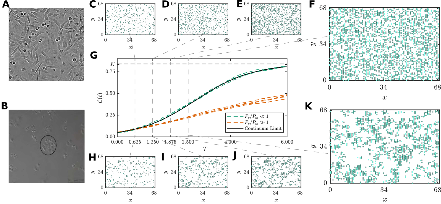
For example, the discrete model formulation can replicate many realistic spatiotemporal patterns observed in cell biology. Figure 1(A),(B) demonstrates typical microscopy images obtained from in vitro cell culture assays; ubiquitous and important experimental techniques used in the study of cell motility, cell proliferation and drug design. Various patterns are observed: prostate cancer cells (PC-3 line) tend to be highly motile, and spread uniformly to invade vacant spaces (Figure 1(A)); in contrast breast cancer cells (MBA-MD-231 line) tend be relatively stationary with proliferation events driving the formation of aggregations (Figure 1(B)). These phenomena may be captured using a lattice-based discrete model framework by varying the ratio where and are, respectively, the probabilities that an agent attempts to proliferate and attempts to move during a time interval of duration (See Section 3.2). For , behavior akin to PC-3 cells is recovered (Figure 1(C)–(F)) (Jin et al., 2016). Setting , as in Figure 1(H)–(K), leads to clusters of occupied lattices sites that are similar to the aggregates of MBA-MD-231 cells (Agnew et al., 2014; Simpson et al., 2013).
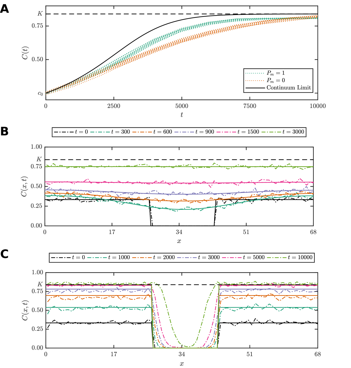
It is common practice to derive approximate continuum-limit differential equation descriptions of discrete models (Callaghan et al., 2006; Jin et al., 2016; Simpson et al., 2010) (Supplementary Material). Such approximations provide a means of performing analysis with significantly reduced computational requirements, since evaluating an exact analytical solution, if available, or otherwise numerically solving a differential equation is typically several orders of magnitude faster than generating a single realization of the discrete model, of which hundreds or thousands may be required for reliable ABC sampling (Browning et al., 2018). However, such approximations are generally only valid within certain parameter regimes, for example here when (Callaghan et al., 2006; Simpson et al., 2010). Consider Figure 1(G), the population density growth curve from the continuum-limit logistic growth model is superimposed with stochastic data for four realizations of a discrete model with and , under initial conditions simulating a proliferation assay, where each lattice site is randomly populated with constant probability, such that there are no macroscopic gradients present at . The continuum-limit logistic growth model is an excellent match for the case (Figure 1(C)–(F)), but severely overestimates the population density when since the mean-field assumptions underpinning the continuum-limit model are violated by the presence of clustering (Figure 1(H)–(K)) (Agnew et al., 2014; Simpson et al., 2013).
As we demonstrate in Section 3, our methods generate accurate ABC posteriors for inference on the discrete problem for a range of biologically relevant parameter regimes, including those where the continuum-limit approximation is poor. In this respect we demonstrate a novel use of approximations that qualitatively respond to changes in parameters in a similar way to the full exact stochastic model.
2 Methods
In this section, we present details of two new algorithms for the acceleration of ABC inference for expensive stochastic models when an appropriate approximation is available. First, we present essential background in ABC inference and sequential Monte Carlo (SMC) samplers for ABC (Sisson et al., 2007; Toni et al., 2009). We then describe our extensions to SMC samplers for ABC and provide numerical examples of our approaches using topical examples from ecology and cell biology.
2.1 Sequential Monte Carlo for Approximate Bayesian computation
Bayesian analysis techniques are powerful tools for the quantification of uncertainty in parameters, models and predictions (Gelman et al., 2014). Unfortunately, for many stochastic models of practical interest, the likelihood function is intractable. ABC methods replace likelihood evaluation with an approximation based on stochastic simulations of the proposed model, this is captured directly in ABC rejection sampling (Pritchard et al., 1999; Tavaré et al., 1997) where samples are generated from an approximate posterior, denoted by . Here is a data generation process based on simulation of the model, is a discrepancy metric, and is the discrepancy threshold. The resulting accepted parameter samples are distributed according to as .
The average acceptance probability of a proposed parameter sample is (Fearnhead and Prangle, 2012), where is the dimensionality of the data space, . This renders rejection sampling computationally expensive or even completely prohibitive, especially for high-dimensional parameter spaces (Marjoram et al., 2003; Sisson et al., 2007). Summary statistics can reduce the data dimensionality, however, they will often incur information loss (Barnes et al., 2012; Blum et al., 2013; Fearnhead and Prangle, 2012). However, strategies including regression adjustment and marginal adjustment strategies can improve the accuracy of dimension reductions (Beaumont et al., 2002; Nott et al., 2014).
In the SMC-ABC method, importance resampling is applied to a sequence of ABC posteriors with discrepancy thresholds , with indicating the target ABC posterior. Given weighted samples , called particles, from the prior , particles are filtered through each ABC posterior using three main steps for each particle : (i) the particle is perturbed using a proposal kernel density ; (ii) an accept/reject step is performed; and (iii) importance weights are updated. Once all particles have been updated and reweighted, resampling of particles is performed to avoid particle degeneracy. For reference, the SMC-ABC algorithm as initially developed by Sisson et al. (2007) and Toni et al. (2009) is given in Algorithm 1. The number of particles, , and the number of intermediate distributions, , influence the accuracy and performance, respectively, of the sampler. Setting too small can lead to large estimator variability and particle degeneracy, and setting too small leads to large divergence between successive distributions that can result in high rejection rates.
Note that throughout all algorithms used in this manuscript, we assume that the initial set of weighted particles, , are independent, identically distributed samples from the prior, , and therefore have uniform weight, , for all . However, the methods are general enough to deal with prior distributions that require importance sampling to draw truly weighted particles.
For a fixed choice of , efficient use of SMC-ABC depends critically on the selection of appropriate proposal kernels and threshold sequences. The process of sampling at the target threshold, , given the weights of the previous threshold, , is described by Filippi et al. (2013)
| (1) |
where the data space, , has dimensionality , is a -dimensional ball centered on the data with radius , and denotes the indicator function with if , otherwise . The normalization constant, , can be interpreted as the average acceptance probability across all particles. We see this by noting that Equation (1) can be reduced to
| (2) |
Here the distribution represent the proposal mechanism,
| (3) |
and is the probability that simulated data is within of the data given a parameter value . Therefore, the normalizing constant is
| (4) |
that is, is the average acceptance probability.
From a computational perspective, the goal is to choose to maximize . However, this would not necessarily result in a that is an accurate approximation to the true target ABC posterior . To achieve this goal, we require such that the Kullback-Leibler divergence (Kullback and Leibler, 1951), , is minimized. Beaumont et al. (2009) and Filippi et al. (2013) demonstrate how the latter goal provides insight into how to optimally choose . The key is to note that can be decomposed as follows,
| (5) | ||||
where is independent of . By rearranging Equation (5), we obtain
That is, minimizing is equivalent to minimizing
and maximizing simultaneously.
Therefore, any proposal mechanism that is closer, in the Kullback-Liebler sense, to is more efficient.
2.2 Preconditioning SMC-ABC
Consider a fixed sequence of ABC posteriors for the stochastic model inference problem, . We want to apply SMC-ABC (Supplementary Material) to efficiently sample from this sequence with adaptive proposal kernels, (Beaumont et al., 2009; Filippi et al., 2013). Our method exploits an approximate model to further improve the average acceptance probability.
2.2.1 Algorithm development
Say we have a set of weighted particles that represent the ABC posterior at threshold using the stochastic model, that is, . Now, consider applying the next importance resampling step using an approximate data generation step, , where is the simulation process of an approximate model222Throughout, the overbar tilde notation, e.g. , is used to refer to the ABC entities related to the approximate model, whereas quantities without the overbar tilde notation, e.g. , are used to refer fo the ABC entities related to the exact model.. Furthermore, assume the computational cost of simulating the approximate model, , is significantly less than the computational cost of the exact model, , that is, . The result will be a new set of particles that represent the ABC posterior at threshold using this approximate model, denoted . As noted in the examples in Section 1, approximate models are not always valid. This implies that is always biased and will not in general converge to as . However, since , it is computationally inexpensive to compute the distribution
| (6) |
in comparison to computing (Equation (3)). In Equation (6), the proposal kernel is possibly distinct from the used in (Equation (3)). To improve the efficiency of the sampling process we simply require
| (7) |
for (Equation (6)) to be more efficient as a proposal mechanism compared with (Equation (3)). Provided the condition holds, any improvements in sampling efficiency will translate directly into computational performance improvements. That is, it does not matter that is biased, it just needs to be less biased than and computationally inexpensive.
This idea yields an intuitive new algorithm for SMC-ABC; proceed through the sequential sampling of by applying two resampling steps for each iteration. The first moves the particles from acceptance threshold to using the computationally inexpensive approximate model, and the second corrects for the bias between and using the expensive stochastic model, but at an improved acceptance rate. Since the intermediate distribution acts on the proposal mechanism to accelerate the convergence time of SMC-ABC, we denote the sequence as the preconditioner distribution sequence. The algorithm, called preconditioned SMC-ABC (PC-SMC-ABC), is given in Algorithm 2. We note that similar notions of preconditioning with approximation informed proposals have been applied in the context of Markov chain Monte Carlo samplers (Parno and Marzouk, 2018). However, to the best of our knowledge, our approach represents the first application of preconditioning ideas to SMC-ABC.
One particular advantage of the PC-SMC-ABC method, that is demonstrated in the next section, is that it is unbiased. Effectively, one can consider PC-SMC-ABC as standard SMC-ABC method with a specialized proposal mechanism based on the preconditioner distribution. This means that PC-SMC-ABC is completely general, as discussed in Section 4, and is independent of the specific stochastic models that we consider here. This property of unbiasedness holds even for cases where the approximate model is a poor approximation of the forward dynamics of the model. However, the closer that is to the better the performance improvement will be, as we demonstrate in Section 3.
2.3 Moment-matching SMC-ABC
The PC-SMC-ABC method is a promising modification to SMC-ABC that can accelerate inference for expensive stochastic models without introducing bias. However, other approaches can be used to obtain further computational improvements. Here, we consider an alternate approach to utilizing approximate models that aims to get the most out of a small sample of expensive stochastic simulations. Unlike PC-SMC-ABC, this method is generally biased, but it has the advantage of yielding a small and fixed computational budget. Specifically, we define a parameter , such that is the target computational speedup, for example, should result in approximate times speedup. We apply the SMC-ABC method using particles based on the approximate model, and then use particles based on the stochastic model to construct a hybrid population of particles that will represent the final inference on the stochastic model. The key idea is that we use the particles of the expensive stochastic model to inform a transformation on the particles of the approximation such that they the emulate particles of expensive stochastic model. Here, and are, respectively, the floor and ceiling functions.
2.3.1 Algorithm development
Assume that we have applied SMC-ABC to sequentially sample particles through the ABC posteriors from the approximate model, , with . For the sake of the derivation, say that for all we have available the mean vector, , and the covariance matrix, , of the ABC posterior under the stochastic model. In this case, we use particles to emulate particles by using the moment matching transform (Lei and Bickel, 2011; Sun et al., 2016)
| (8) |
where and are the empirical mean vector and convariance matrix of particles , and are lower triangular matrices obtained through the Cholesky factorization (Press et al., 1997) of and , respectively, and is the matrix inverse of . This transform will produce a collection of particles that has a sample mean vector of and covariance matrix . That is, the transformed sample matches the ABC posterior under the stochastic model up to the first two moments. In Section 3, we demonstrate that matching two moments is sufficient for the problems we investigate here, however, in principle we could extend this matching to higher order moments if required. For discussion on the advantages and disadvantages of matching higher moments, see Section 4.
In practice, it would be rare that and are known. If is available, then we can use importance resampling to obtain particles, , from , that is, we perform a step from SMC-ABC using the expensive stochastic model. We can then use the unbiased estimators
| (9) |
to obtain estimates of and . Substituting Equation (9) into Equation (8) gives an approximate transform
| (10) |
where . This enables us to construct an estimate of by applying the moment-matching transform (Equation (10)) to the particles then pooling the transformed particles with the particles that were used in the estimates and . The goal of the approximate transform application is for the transforms particles to be more accurate in higher moments due, despite only matching the first two moments (see Section 3.6 for numerical justification of this property for some specific examples). This results in an approximation of using a set of particles with where .
This leads to our moment-matching SMC-ABC (MM-SMC-ABC) method. First, SMC-ABC inference is applied using the approximate model with particles. Then, given samples from the prior, , we can sequentially approximate
. At each iteration the following steps are performed: (i) generate a small number of particles from using importance resampling and stochastic model simulations; (ii) compute and ; (iii) apply the transform from Equation (10) to the particles at from the approximate model; (iv) pool the resulting particles with the stochastic model samples; and (v) reweight particles and resample.
The final MM-SMC-ABC algorithm is provided in Algorithm 3.
The performance of this method depends on the choice of . Note that in Algorithm 3, standard SMC-ABC for the expensive stochastic model is recovered as
(no speedup, inference unbiased), and standard SMC-ABC using the approximate model is recovered as (maximum speedup, but inference biased). Therefore we expect there is a choice of that provides an optimal trade-off between computational improvement and accuracy. Clearly, the expected speed improvement is proportional to , however, if is chosen to be too small, then the statistical error in the estimates in Equation (9) will be too high. We explore this trade-off in detail in Section 3.6 and find that seems to give a reasonable result.
3 Results
In this section, we provide numerical examples to demonstrate the accuracy and performance of the PC-SMC-ABC and MM-SMC-ABC methods. First we apply PC-SMC-ABC to a tractable example to demonstrate the mechanisms of the method and provide insight into effective choices of approximate model. The tractable example considered here is inference for an Ornstein–Uhlenbeck process (Uhlenbeck and Ornstein, 1930). We then consider two intractable problems based on expensive discrete model. For our first example, we consider the analysis of spatially averaged population growth data. The discrete model used in this instance is relevant in the ecological sciences as it describes population growth subject to a weak Allee effect (Taylor and Hastings, 2005). We then analyze data that is typical of in vitro cell culture scratch assays in experimental cell biology using a discrete model that leads to the well-studied Fisher-KPP model (Edelstein-Keshet, 2005; Murray, 2002). In both examples, we present the discrete model and its continuum limit, then compute the full Bayesian posterior for the model parameters using the PC-SMC-ABC (Algorithm 2) and MM-SMC-ABC (Algorithm 3) methods, and compare the results with the SMC-ABC (Supplementary Material) using either the discrete model or continuum limit alone. We also provide numerical experiments to evaluate the effect of the tuning parameter on the accuracy and performance of the MM-SMC-ABC method.
It is important to clarify that when we refer to the accuracy of our methods, we refer to their ability to sample from the target ABC posterior under the expensive stochastic model. The evaluation of this accuracy requires sampling from the target ABC posterior under the expensive stochastic model using SMC-ABC. As a result, the target acceptance thresholds are chosen to ensure this is computationally feasible.
3.1 A tractable example: Ornstein–Uhlenbeck process
The Ornstein–Uhlenbeck process is a mean reverting stochastic process with many applications in finance, biology and physics (Uhlenbeck and Ornstein, 1930). The evolution of the continuous state is given by an Itō stochastic differential equation (SDE) of the form
| (11) |
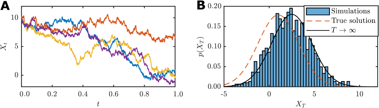
where is the long-term mean, is the rate of mean reversion, is the process volatility, is a Wiener process and is a constant initial condition. Example realisations are shown in Figure 2(A).
We consider data consisting of independent realisations of the Ornstein–Uhlenbeck processs at time , that is, . This inference problem is analytically tractable since the Fokker–Planck equation can be solved to obtain a Gaussian distribution for the data,
| (12) |
For demonstration purposes we will assume a solution for the full Fokker–Planck equation is unavailable and perform ABC inference to estimate the volatility parameter, , using stochastic simulation with the Euler–Maruyama discretisation (Maruyama, 1955),
| (13) |
where is a standard normal variate and is a small time step. For the approximate model we take the stationary distribution of the Ornstein–Uhlenbeck process obtained by taking and solving the steady state of the Fokker–Planck equation,
| (14) |
This kind of approximation will often be possible since the steady state Fokker–Planck equation is more likely to be tractable than the transient solution for most SDE models. As shown in Figure 2(B), the stationary solution is a better approximation for the true variance than for the true mean. Therefore, for small this approximation would be more appropriate as a preconditioner for inference of the volatility parameter, , in Equation (11) than for the long-time mean, . In general, the performance expected from preconditioning will increase as increases since the stationary approximation will become more accurate (Supplementary Material).
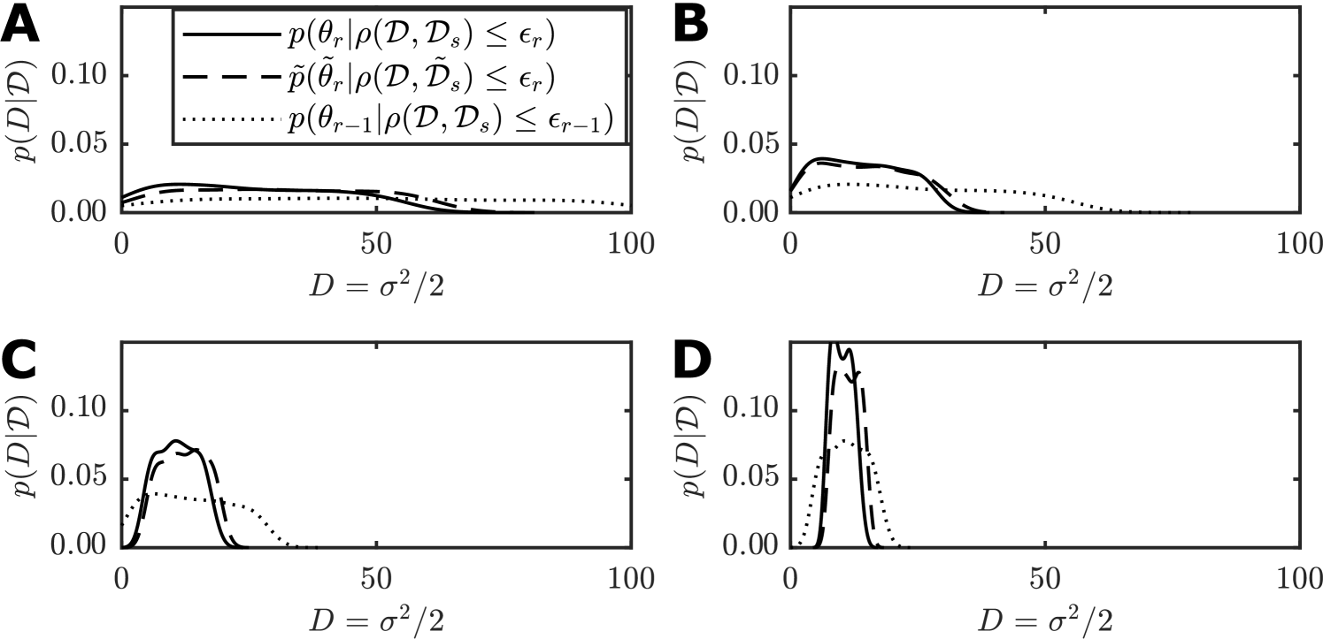
Figure 3 demonstrates th results of applying PC-ABC-SMC (Algorithm 2) with particles, showing intermediate distributions, for inferring given data at , using stochastic simulation for the exact model (Equation (13)) with , and the stationary distribution (Equation (14)) for the approximate model used in the preconditioning step.
In this example, all other parameters are treated as known with , and . Data is generated using as in Figure 2. In each step, the preconditioner distribution for threshold (dashed line) is a better proposal distribution for the target (solid line) than that of the exact model at threshold (dotted line). The overall speedup factor is approximately for this example, and it continues to improve as increases since Equation (14) becomes an increasingly better approximation to Equation (12) (See Supplementary Material). For truly intractable problems, such as the lattice-based random walk models presented in Sections 3.4 and 3.5, we obtain superior performance gains of up to a factor of four.
3.2 Lattice-based stochastic discrete random walk model
The stochastic discrete model we consider is a lattice-based random walk model that is often used to describe populations of motile cells (Jin
et al., 2016). The model involves initially placing a population of agents of size on a lattice, (Callaghan
et al., 2006; Simpson
et al., 2010), for example an hexagonal lattice (Jin
et al., 2016). This hexagonal lattice is defined by a set of indices
, and a neighborhood function,
Lattice indices are mapped to Cartesian coordinates using
| (15) |
We define an occupancy function such that if site is occupied by an agent at time , otherwise . This means that in our discrete model each lattice site can be occupied by, at most, one agent.
During each discrete time step of duration , agents attempt to move with probability and attempt to proliferate with probability . If an agent at site attempts a motility event, then a neighboring site will be selected uniformly at random. The motility event is aborted if the selected site is occupied, otherwise the agent will move to the selected site (Figure 4(A)–(C)).
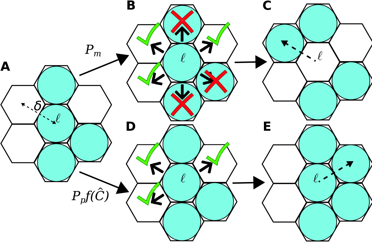
For proliferation events, the local neighborhood average occupancy,
is calculated and a uniform random number is drawn. If , where is called the crowding function (Browning et al., 2017; Jin et al., 2016), then the proliferation event is aborted due to local crowding effects and contact inhibition. If , then proliferation is successful and a daughter agent is placed at a randomly chosen unoccupied lattice site in (Figure 4(A),(D)–(E)). The evolution of the model is generated through repeating this process though time steps, . This approach, based on the work by Jin et al. (2016), supports a generic proliferation mechanism since is an arbitrary smooth function satisfying and , where is the carrying capacity density. However, in the literature there are also examples that include other mechanisms such as cell-cell adhesion (Johnston et al., 2013), directed motility (Binny et al., 2016), and Allee effects (Böttger et al., 2015).
3.3 Approximate continuum-limit descriptions
Discrete models do not generally lend themselves to analytical methods, consequently, their application is intrinsically tied to computationally intensive stochastic simulations and Monte Carlo methods (Jin et al., 2016). As a result, it is common practice to approximate mean behavior using differential equations by invoking mean-field assumptions, that is, to treat the occupancy status of lattice sites as independent (Callaghan et al., 2006; Simpson et al., 2010). The resulting approximate continuum-limit descriptions (Supplementary Material) are partial differential equations (PDEs) of the form
| (16) |
where , is the diffusivity, is the proliferation rate with , and is the crowding function that is related to the proliferation mechanism implemented in the discrete model (Browning et al., 2017; Jin et al., 2016). For spatially uniform populations there will be no macroscopic spatial gradients on average, that is . Thus, is just a function of time, , and the continuum limit reduces to an ordinary differential equation (ODE) describing the net population growth,
| (17) |
For many standard discrete models, the crowding function is implicitly (Callaghan et al., 2006). That is, the continuum limits in Equation (16) and Equation (17) yield the Fisher-KPP model (Edelstein-Keshet, 2005; Murray, 2002) and the logistic growth model (Tsoularis and Wallace, 2002; Warne et al., 2017), respectively. However, non-logistic growth models , for example, for , have also been considered (Jin et al., 2016; Simpson et al., 2010; Tsoularis and Wallace, 2002).
3.4 Temporal example: a weak Allee model
The Allee effect refers to the reduction in growth rate of a population at low densities. This is particularly well studied in ecology where there are many mechanisms that give rise to this phenomenon (Taylor and Hastings, 2005; Johnston et al., 2017). We introduce an Allee effect into our discrete model by choosing a crowding function of the form
where is the local density at the lattice site , at time , is the carrying capacity density, and is the Allee parameter which yields a weak Allee effect for (Wang et al., 2019). Note that smaller values of entail a more pronounced Allee effect with leading to a strong Allee effect that can lead to species extinction (Wang et al., 2019). For simplicity, we only consider the weak Allee effect here, but our methods are general enough to consider any sufficiently smooth .
Studies in ecology often involve population counts of a particular species over time (Taylor and Hastings, 2005). In the discrete model, the initial occupancy of each lattice site is independent, and hence there are no macroscopic spatial gradients on average. It is reasonable to summarize simulations of the discrete model at time by the average occupancy over the entire lattice, . Therefore, the continuum limit for this case is given by (Wang et al., 2019)
| (18) |
with , , and .
We generate synthetic time-series ecological data using the discrete model, with observations made at times , resulting in data with where is the average occupancy at time for a single realization of the discrete model (Supplementary Material). For this example, we consider an hexagonal lattice with , , and parameters , , , , and . Reflecting boundary conditions are applied at all boundaries and a uniform initial condition is applied, specifically, each site is occupied with probability for all , giving . This combination of parameters is selected since it is known that the continuum limit (Equation (18)) will not accurately predict the population growth dynamics of the discrete model in this regime since (Supplementary Material).
For the inference problem we assume is known, and we seek to compute under the discrete model with and . We utilize uninformative priors, , and with the additional constraint that , that is, and are not independent in the prior. The discrepancy metric used is the Euclidean distance. For the discrete model, this is
where is the average occupancy at time of a realization of the discrete model given . Similarly, for the continuum limit we have
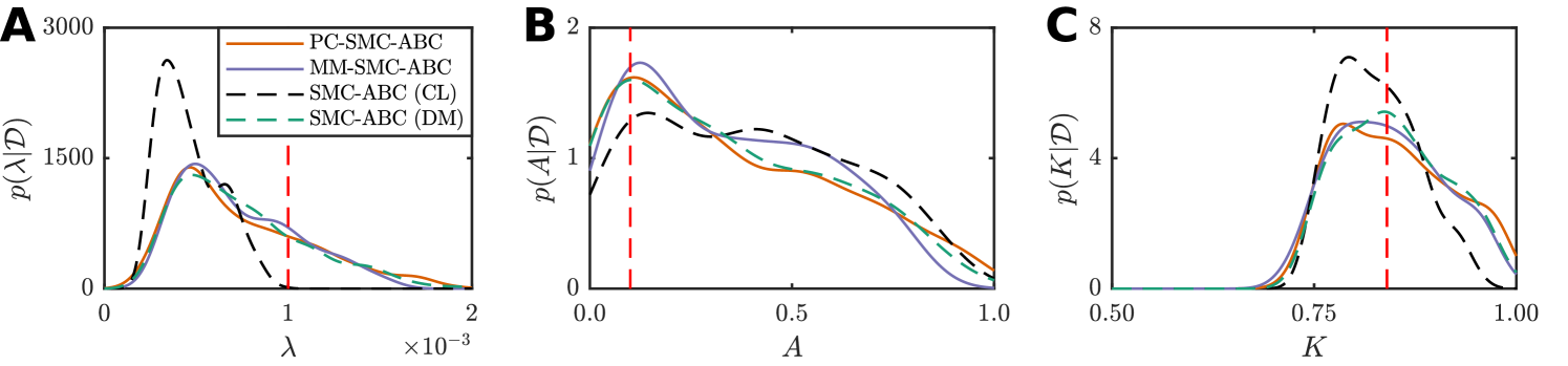
where is the solution to the continuum limit (Equation (18)), computed numerically (Supplementary Material). We compute the posterior using our PC-SMC-ABC and MM-SMC-ABC methods to compare with SMC-ABC under the continuum limit and SMC-ABC under the discrete model. In each instance, particles are used to approach the target threshold using the sequence with . In the case of MM-SMC-ABC the tuning parameter is . The Gaussian proposal kernels, and , are selected adaptively (Fehlberg, 1969; Iserles, 2008) (Supplementary Material).
Figure 5 and Table 1 present the results. SMC-ABC using the continuum-limit model is a poor approximation for SMC-ABC using the discrete model, especially for the proliferation rate parameter, (Figure 5(a)), which is expected because . However, the posteriors estimated using PC-SMC-ABC are an excellent match to the target posteriors estimated using SMC-ABC with the expensive discrete model, yet the PC-SMC-ABC method requires only half the number of stochastic simulations (Table 1). The MM-SMC-ABC method is not quite as accurate as the PC-SMC-ABC method, however, the number of expensive stochastic simulations is reduced by more than a factor of eight (Table 1) leading to considerable increase in computational efficiency.
| Method | Stochastic samples | Continuum samples | Run time (hours) | Speedup |
|---|---|---|---|---|
| SMC-ABC | ||||
| PC-SMC-ABC | ||||
| MM-SMC-ABC |
3.5 Spatiotemporal example: a scratch assay
We now look to a discrete model commonly used in studies of cell motility and proliferation, and use spatially extended data that is typical of in vitro cell culture experiments, specifically scratch assays (Liang et al., 2007).
In this case we use a crowding function of the form , where is the carrying capacity density, since it will lead to a logistic growth source term in Equation (16) which characterizes the growth dynamics of many cell types (Simpson et al., 2010; Warne et al., 2017). The discrete model is initialized such that initial density is independent of . Therefore, we summarize the discrete simulation by computing the average occupancy for each coordinate, that is, we average over the -axis in the hexagonal lattice (Jin et al., 2016), that is, . Thus, one arrives at the Fisher-KPP model (Edelstein-Keshet, 2005; Murray, 2002) for the continuum limit,
| (19) |
where , , and .
Just as with the weak Allee model, here we generate synthetic spatiotemporal cell culture data using the discrete model. Observations are made at times , resulting in data
with where is the average occupancy over sites at time for a single realization of the discrete model. As with the weak Allee model, we consider an hexagonal lattice with , , and parameters , , and . We simulate a scratch assay by specifying the center 20 cell columns () to be initially unoccupied, and apply a uniform initial condition outside the scratch area such that overall. Reflecting boundary conditions are applied at all boundaries. Note, we have selected a parameter regime with for which the continuum limit is an accurate representation of the discrete model average behavior (Supplementary Material).
Since we have spatial information for this problem, we assume is also an unknown parameter and perform inference on the discrete model to compute with
, , and . We utilize uninformative priors,
, , and . For the discrepancy metric we use the Frobenius norm; for the discrete model, this is
where is the average occupancy at site at time of a realization of the discrete model given parameters . Similarly, for the continuum limit we have
where is the solution to the continuum-limit PDE (Equation (19)), computed using a backward-time, centered-space finite difference scheme with fixed-point iteration and adaptive time steps (Simpson et al., 2007; Sloan and Abbo, 1999) (Supplementary Material). We estimate the posterior using our PC-SMC-ABC and MM-SMC-ABC methods to compare with SMC-ABC using the continuum limit and SMC-ABC using the discrete model. In each case, particles are used to approach the target threshold, , using the sequence with . In the case of MM-SMC-ABC the tuning parameter is . Again, Gaussian proposal kernels, and , are selected adaptively (Supplementary Material).
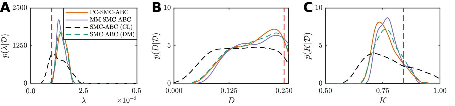
Results are shown in Figure 6 and Table 2. Despite the continuum limit being a good approximation of the discrete model average behavior, using solely this continuum limit in the inference problem still leads to bias. Just as with the weak Allee model, both PC-SMC-ABC and MM-SMC-ABC methods produce a more accurate estimate of the SMC-ABC posterior density with the discrete model. Overall, PC-SMC-ABC is unbiased, however, MM-SMC-ABC is still very accurate. The main point for our work is that the PC-SMC-ABC and MM-SMC-ABC methods both produce posteriors that are accurate compared with the expensive stochastic inference problem, whereas the approximate model alone does not. From Table 2, both PC-SMC-ABC and MM-SMC-ABC require a reduced number of stochastic simulations of the discrete model compared with direct SMC-ABC. For PC-SMC-ABC, the reduction is almost a factor of four and, for MM-SMC-ABC, the reduction is almost a factor of eleven.
| Method | Stochastic samples | Continuum samples | Run time (hours) | Speedup |
|---|---|---|---|---|
| SMC-ABC | ||||
| PC-SMC-ABC | ||||
| MM-SMC-ABC |
3.6 A guide to selection of for MM-SMC-ABC
The performance of MM-SMC-ABC is dependent on the tuning parameter . Since MM-SMC-ABC will only propagate particles based on the expensive stochastic model, can be considered as a target computational cost reduction factor with being the target speed up factor. However, intuitively there will be a limit as to how small one can choose before the statistical error incurred from the estimates of and is large enough to render the approximate moment matching transform inaccurate. It is non-trivial to analyze MM-SMC-ABC to obtain a theoretical guideline for choosing , therefore we perform a computational benchmark to obtain a heuristic. It should be noted that we use an SMC-ABC sampler with as a benchmark for accuracy and performance. As a result, it may be that repeating the analysis with larger could lead to a smaller optimal .
Here, using different values for we repeatedly solve the weak Allee model (Section 3.4) and the scratch assay model (Section 3.5). For both inverse problems we applied MM-SMC-ABC under identical conditions as in Sections 3.4 and 3.5 with the exception of the tuning parameter that takes values from the sequence with and for . For each in the sequence, we consider independent applications of MM-SMC-ABC. The computational cost for each is denoted by and represents the run time in seconds for an application of MM-SMC-ABC with tuning parameter . We also calculate an error metric,
where is a set of particles from an application of SMC-ABC using the expensive stochastic model, and is the pooled exact and approximate transformed particles from the th application of MM-SMC-ABC. For , the function is the -th order empirical moment-matching distance function (Liao et al., 2015; Lillacci and Khammash, 2010; Zechner et al., 2012), given by
for two sample sets and with for , and . For any -dimensional discrete vector , then is the th empirical raw moment of the sample
set ,
where . Note that must be greater than the number of moments that are matched in the approximate transform (Equation (10)) to ensure that MM-SMC-ABC is improving the accuracy in higher moments also.
We estimate the average and for each value of for both the weak Allee effect and the scratch assay inverse problems. Figure 7 displays the estimates and standard errors given and , with the value of shown. We emphasize that , that is our error measure compares the first six moments while only two moments are matched.
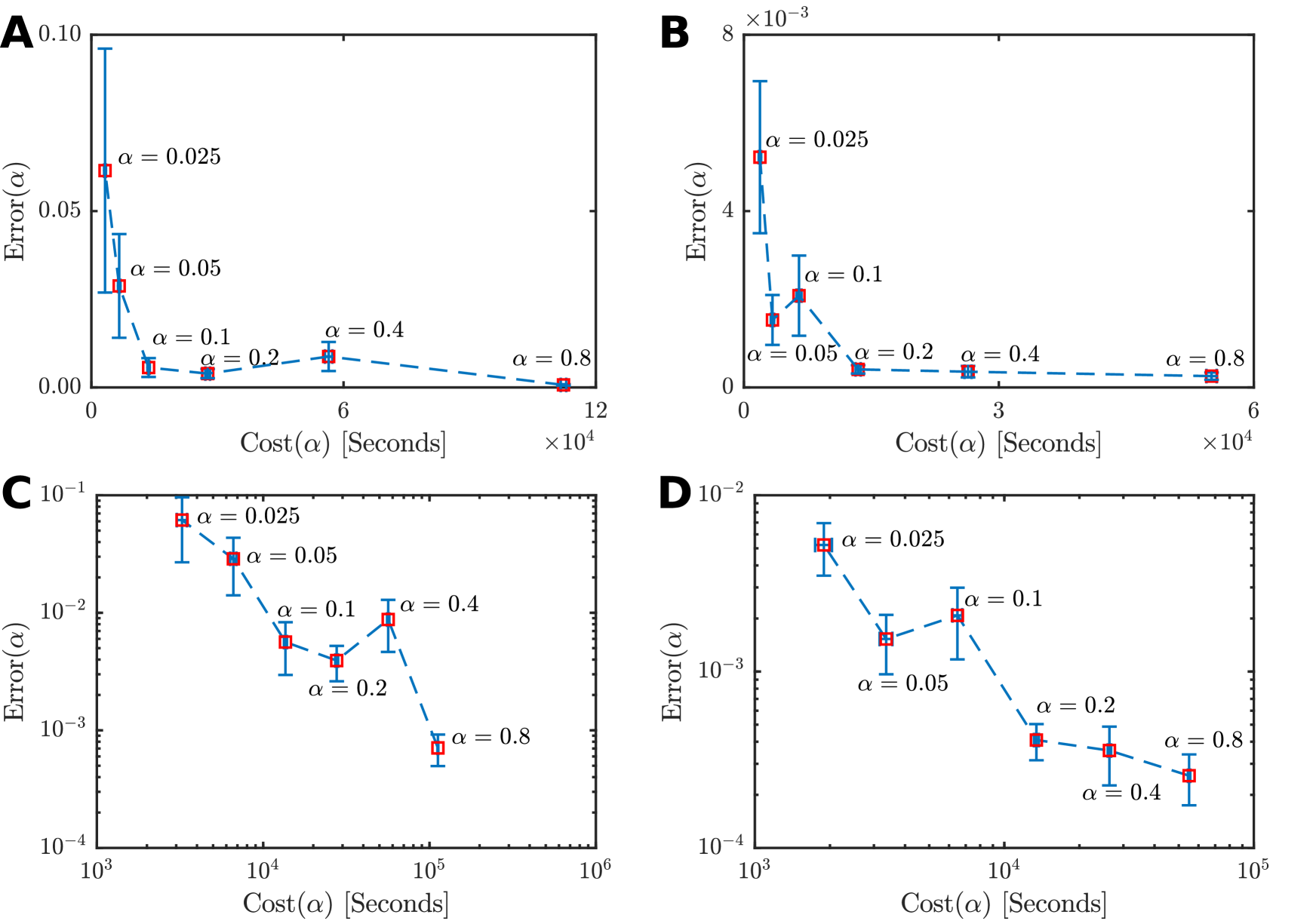
There is clearly a threshold for , below which the error becomes highly variable. For both the weak Allee effect model (Figure 7(A),(C)) and the scratch assay model (Figure 7(B),(D)), the optimal choice of is located between and . Therefore, we suggest a heuristic of to be a reliable choice. If extra performance is needed may also be acceptable, but if accuracy is of the utmost importance then seems to be the most robust choice. This experiment also provides insight in to the consistency and stability of the MM-SMC-ABC method, where leads to results that are consistently fast and have low variability in the error metric. While further work is required to assess theoretically the stability and consistency properties of this method, these numerical results are promising. In general, the choice of optimal is still an open problem and is likely to be impacted by the specific nature of the relationship between the exact model and the approximate model.
3.7 Summary
This section presented numerical examples to demonstrate our new methods, PC-SMC-ABC and MM-SMC-ABC, for ABC inference with expensive stochastic discrete models. The tractable Ornstein–Uhlenbeck process was used to highlight the mechanisms leading to the performance improvements of PC-ABC-SMC. Then two examples based on lattice-based random walks were used to demonstrate the efficacy of both PC-SMC-ABC and MM-SMC-AB. In the weak Allee model example, data were generated using parameters that violate standard continuum-limit assumptions; in the scratch assay model example, the Fisher-KPP continuum limit is known to be a good approximation in the parameter regime of the generated data. In both examples, final inferences are biased when the continuum limit is exclusively relied on in the SMC-ABC sampler. However, the results from our new algorithms, PC-SMC-ABC and MM-SMC-ABC, show significantly more accurate posteriors can be computed at a fraction of the cost of the full SMC-ABC using the discrete model, with speed improvements over an order of magnitude.
As mentioned in Section 2.3, the tuning parameter, , in the MM-SMC-ABC method effectively determines the trade-off between the computational speed of the approximate model and the accuracy of the expensive stochastic model. The values and correspond to performing inference exclusively with, respectively, the continuum limit and the stochastic discrete model. Based on numerical experimentation, we find that is quite reasonable, however, this conclusion will be dependent on the specific model, the parameter space dimensionality, and the number of particles used for the SMC scheme.
4 Discussion
In the life sciences, computationally challenging stochastic discrete models are routinely used to characterize the dynamics of biological populations (Codling et al., 2008; Callaghan et al., 2006; Simpson et al., 2010). In practice, approximations such as the mean-field continuum limit are often derived and used in place of the discrete model for analysis and, more recently, for inference. However, parameter inferences will be biased when the approximate model is solely utilized for inference, even in cases when the approximate model provides an accurate description of the average behaviour of the stochastic model.
We provide a new approach to inference for stochastic models that maintains all the methodological benefits of working with discrete mathematical models, while avoiding the computational bottlenecks of relying solely upon repeated expensive stochastic simulations. Our two new algorithms, PC-SMC-ABC and MM-SMC-ABC, utilize samples from the approximate model inference problem in different ways to accelerate SMC-ABC sampling. The PC-SMC-ABC method is asymptotically unbiased, and we demonstrate computational improvements of up to a factor of almost four are possible. While potentially biased, MM-SMC-ABC can provide further improvements. In general, the expected speedup is around , and is reasonable based on our numerical investigations. For larger values of it may be that even smaller values of could be effective.
There are some assumptions in our approach that could be generalized in future work. First, in PC-SMC-ABC, we assume that the condition in Equation (7) holds for all ; this is reasonable for the models we consider since we never observe a decrease in performance. However, it may be possible for the bias in the approximate model to be so extreme for some that the condition in Equation (7) is violated, leading to a decrease in performance at specific generations. Acceptance probabilities could be estimated by performing a small set of trial samples from both and proposal mechanisms, enabling automatic selection of the optimal proposal mechanism. Second, in the moment matching transform proposed in Equation (8), we use two moments only as this is sufficient for the problems we consider here with numerical examples demonstrating accuracy in the first six moments. However, our methodology is sufficiently flexible that additional moments can be incorporated if necessary. While including higher moments will improve the accuracy of the moment-matching transform, more samples from the exact model will be required to achieve initial estimates of these moments resulting in eroded performance.
While the performance improvements we demonstrate here are significant, it is also possible to obtain improvements of similar order through detailed code optimization techniques applied to standard SMC-ABC. We emphasize that our schemes would also benefit from such optimizations as advanced vectorization and parallelization to further improve their performance (Lee et al., 2010; Warne et al., 2021). Our algorithm extensions are also more direct to implement over advanced high performance computing techniques for acceleration of computational schemes.
There are many extensions to our methods that could be considered. We have based our presentation on a form of an SMC-ABC sampler that uses a fixed sequence of thresholds. However, the ideas of using the preconditioning distribution, as in PC-SMC-ABC, and the moment matching transform, as in MM-SMC-ABC, are applicable to SMC schemes that adaptively select thresholds (Drovandi and Pettitt, 2011). Recently, there have been a number of state-of-the-art inference schemes introduced based on multilevel Monte Carlo (MLMC) (Giles, 2015; Warne et al., 2019a). Our new SMC-ABC schemes could exploit MLMC to combine samples from all acceptance thresholds using a coupling scheme and bias correction telescoping summation, such as in the work of Jasra et al. (2019) or Warne et al. (2018). Early accept/rejection schemes, such as those considered by Prangle (2016), Prescott and Baker (2020), and Lester (2020), could also be introduced for the sampling steps involving the expensive discrete model. Lastly, the PC-SMC-ABC and the MM-SMC-ABC methods could also be applied together and possibly lead to a compounding effect in the performance. Delayed acceptance schemes (Banterle et al., 2019; Everitt and Rowińska, 2020; Golightly et al., 2015) are also an alternative approach with similar motivations to the methods we propose in this work. However, these approaches can be highly sensitive to false negatives, that is, cases where a particular value of would be rejected under the approximate model but accepted under the exact model . Our PC-SMC-ABC approach is not affected by false negatives due to the use of the second set of proposal kernels.
We have demonstrated our methods using a two-dimensional lattice-based discrete random-walk model that leads to mean-field continuum-limit approximations with linear diffusion and a source term of the form . However, our methods are more widely applicable. We could further generalize the model to deal with a more general class of reaction-diffusion continuum limits involving nonlinear diffusion (Warne et al., 2019b; Witelski, 1995) and generalized proliferation mechanisms (Simpson et al., 2013; Tsoularis and Wallace, 2002). Our framework is also relevant to lattice-free discrete models (Codling et al., 2008; Browning et al., 2018) and higher dimensional lattice-based models (Browning et al., 2019); we expect the computational improvements will be even more significant in this case. Many other forms of model combinations are also be possible. For example, a sequence of continuum models of increasing complexity could be considered, as in Browning et al. (2019). Alternatively, a sequence of numerical approximations of increasing accuracy could be used for inference using a complex target PDE model (Cotter et al., 2010). Linear mapping approximations of higher order chemical reaction network models, such as in Cao and Grima (2018), could also exploit our approach. Another relevant and very general application in systems biology is utilize reaction rate equations, that are deterministic ODEs, as approximations to stochastic chemical kinetics models (Higham, 2008; Wilkinson, 2009).
Of course, not all approximate models will necessarily provide performance improvements. As demonstrated for the Ornstein–Uhlenbeck example (Section 3.1), the stationary distribution will be more appropriate for inference of rather than with the approximation improving as the model sample time increases. However, as shown for lattice-based random walk models (Sections 3.4 and 3.5), even when the assumptions associated with the approximation do not hold, it is still possible to improve sampling with PC-SMC-ABC and MM-ABC-SMC. Therefore, we suggest that approximations that are derived from some limiting, averaged behavior of the exact model will be good initial candidates for our methods. Semi-automated model reduction techniques also are potential approaches to obtain approximations (Transtrum and Qiu, 2014) that could be investigated in the future.
In this work, novel methods have been presented for exploiting approximate models to accelerate Bayesian inference for expensive stochastic models. We have shown that, even when the approximation leads to biased parameter inferences, it can still inform the proposal mechanisms for ABC samplers using the stochastic model. Our numerical examples show performance improvements of more than tenfold. These substantial computational improvements are promising and expands the feasibility of Bayesian analysis for problems involving expensive stochastic models.
Software availability
Numerical examples presented in this work are available from GitHub
https://github.com/ProfMJSimpson/Warne_RapidBayesianInference_2019.
Acknowledgements
This work was supported by the Australian Research Council (DP170100474). D.J.W. and M.J.S. acknowledge continued support from the Centre for Data Science at the Queensland University of Technology. D.J.W. and M.J.S. are members of the Australian Research Council Centre of Excellence for Mathematical and Statistical Frontiers. R.E.B. would like to thank the Leverhulme Trust for a Leverhulme Research Fellowship, the Royal Society for a Wolfson Research Merit Award, and the BBSRC for funding via BB/R00816/1. M.J.S. appreciates support from the University of Canterbury Erskine Fellowship. Computational resources where provided by the eResearch Office, Queensland University of Technology. The authors thank Wang Jin for helpful discussions.
References
- Agnew et al. (2014) Agnew, D., J. Green, T. Brown, M. Simpson, and B. Binder (2014). Distinguishing between mechanisms of cell aggregation using pair-correlation functions. Journal of Theoretical Biology 352, 16–23.
- Baker et al. (2018) Baker, R. E., J.-M. Peña, J. Jayamohan, and A. Jérusalem (2018). Mechanistic models versus machine learning, a fight worth fighting for the biological community? Biology Letters 14(5), 20170660.
- Banterle et al. (2019) Banterle, M., C. Grazian, A. Lee, and C. P. Robert (2019). Accelerating Metropolis-Hastings algorithms by delayed acceptance. Foundations of Data Science 1(2), 103–128.
- Barnes et al. (2012) Barnes, C. P., S. Filippi, M. P. H. Stumpf, and T. Thorne (2012). Considerate approaches to constructing summary statistics for ABC model selection. Statistics and Computing 22(6), 1181–1197.
- Beaumont et al. (2009) Beaumont, M. A., J.-M. Cornuet, J.-M. Marin, and C. P. Robert (2009). Adaptive approximate Bayesian computation. Biometrika 96(4), 983–990.
- Beaumont et al. (2002) Beaumont, M. A., W. Zhang, and D. J. Balding (2002). Approximate Bayesian computation in population genetics. Genetics 162(4), 2025–2035.
- Binny et al. (2016) Binny, R. N., P. Haridas, A. James, R. Law, M. J. Simpson, and M. J. Plank (2016). Spatial structure arising from neighbour-dependent bias in collective cell movement. PeerJ 4, e1689.
- Black and McKane (2012) Black, A. J. and A. J. McKane (2012). Stochastic formulation of ecological models and their applications. Trends in Ecology & Evolution 27(6), 337–345.
- Blum et al. (2013) Blum, M. G. B., M. A. Nunes, D. Prangle, and S. A. Sisson (2013). A comparative review of dimension reduction methods in approximate Bayesian computation. Statistical Science 28(2), 189–208.
- Böttger et al. (2015) Böttger, K., H. Hatzikirou, A. Voss-Böhme, E. A. Cavalcanti-Adam, M. A. Herrero, and A. Deutsch (2015). An emerging Allee effect is critical for tumor initiation and persistence. PLOS Computational Biology 11(9), e1004366.
- Browning et al. (2019) Browning, A. P., P. Haridas, and M. J. Simpson (2019). A Bayesian sequential learning framework to parameterise continuum models of melanoma invasion into human skin. Bulletin of Mathematical Biology 81(3), 676–698.
- Browning et al. (2018) Browning, A. P., S. W. McCue, R. N. Binny, M. J. Plank, E. T. Shah, and M. J. Simpson (2018). Inferring parameters for a lattice-free model of cell migration and proliferation using experimental data. Journal of Theoretical Biology 437, 251–260.
- Browning et al. (2017) Browning, A. P., S. W. McCue, and M. J. Simpson (2017). A Bayesian computational approach to explore the optimal duration of a cell proliferation assay. Bulletin of Mathematical Biology 79(8), 1888–1906.
- Buzbas and Rosenberg (2015) Buzbas, E. O. and N. A. Rosenberg (2015). AABC: Approximate approximate Bayesian computation for inference in population-genetic models. Theoretical Population Biology 99, 31–42.
- Callaghan et al. (2006) Callaghan, T., E. Khain, L. M. Sander, and R. M. Ziff (2006). A stochastic model for wound healing. Journal of Statistical Physics 122(5), 909–924.
- Cao and Grima (2018) Cao, Z. and R. Grima (2018). Linear mapping approximation of gene regulatory networks with stochastic dynamics. Nature Communications 9(1), 3305.
- Chen and Zhang (2014) Chen, C. P. and C.-Y. Zhang (2014). Data-intensive applications, challenges, techniques and technologies: a survey on Big Data. Information Sciences 275, 314–347.
- Chkrebtii et al. (2015) Chkrebtii, O. A., E. K. Cameron, D. A. Campbell, and E. M. Bayne (2015). Transdimensional approximate Bayesian computation for inference on invasive species models with latent variables of unknown dimension. Computational Statistics & Data Analysis 86, 97–110.
- Codling et al. (2008) Codling, E. A., M. J. Plank, and S. Benhamou (2008). Random walk models in biology. Journal of The Royal Society Interface 5(25), 813–834.
- Cotter et al. (2010) Cotter, S. L., M. Dashti, and A. M. Stuart (2010). Approximation of Bayesian inverse problems for PDEs. SIAM Journal on Numerical Analysis 48(1), 322–345.
- Coveney et al. (2016) Coveney, P. V., E. R. Dougherty, and R. R. Highfield (2016). Big data need big theory too. Philosophical Transactions of the Royal Society A: Mathematical, Physical and Engineering Sciences 374(2080), 20160153.
- DeAngelis and Grimm (2014) DeAngelis, D. L. and V. Grimm (2014). Individual-based models in ecology after four decades. F1000Prime Reports 6, 39.
- Del Moral et al. (2006) Del Moral, P., A. Doucet, and A. Jasra (2006). Sequential Monte Carlo samplers. Journal of the Royal Statistical Society: Series B (Statistical Methodology) 68(3), 411–436.
- Drawert et al. (2017) Drawert, B., M. Griesemer, L. R. Petzold, and C. J. Briggs (2017). Using stochastic epidemiological models to evaluate conservation strategies for endangered amphibians. Journal of The Royal Society Interface 14(133), 20170480.
- Drovandi and Pettitt (2011) Drovandi, C. C. and A. N. Pettitt (2011). Estimation of parameters for macroparasite population evolution using approximate Bayesian computation. Biometrics 67(1), 225–233.
- Edelstein-Keshet (2005) Edelstein-Keshet, L. (2005). Mathematical Models in Biology. Society for Industrial and Applied Mathematics.
- Ellison (2004) Ellison, A. M. (2004). Bayesian inference in ecology. Ecology Letters 7(6), 509–520.
- EHT Collaboration et al. (2019) EHT Collaboration et al. (2019). First M87 Event Horizon Telescope results. VI. the shadow and mass of the central black hole. The Astrophysical Journal Letters 875(1), L6.
- Everitt and Rowińska (2020) Everitt, R. G. and P. A. Rowińska (2020). Delayed acceptance ABC-SMC. Journal of Computational and Graphical Statistics.
- Fearnhead and Prangle (2012) Fearnhead, P. and D. Prangle (2012). Constructing summary statistics for approximate Bayesian computation: semi-automatic approximate Bayesian computation. Journal of the Royal Statistical Society: Series B (Statistical Methodology) 74(3), 419–474.
- Fehlberg (1969) Fehlberg, E. (1969). Low-order classical Runge-Kutta formulas with step size control and their application to some heat transfer problems. Technical Report R-315, NASA.
- Filippi et al. (2013) Filippi, S., C. P. Barnes, J. Cornebise, and M. P. H. Stumpf (2013). On optimality of kernels for approximate Bayesian computation using sequential Monte Carlo. Statistical Applications in Genetics and Molecular Biology 12(1), 87–107.
- Gelman et al. (2014) Gelman, A., J. B. Carlin, H. S. Stern, D. B. Dunson, A. Vehtari, and D. B. Rubin (2014). Bayesian Data Analysis (3rd ed.). Chapman & Hall/CRC.
- Giles (2015) Giles, M. B. (2015). Multilevel Monte Carlo methods. Acta Numerica 24, 259–328.
- Golightly et al. (2015) Golightly, A., D. A. Henderson, and C. Sherlock (2015). Delayed acceptance particle MCMC for exact inference in stochastic kinetic models. Statistics and Computing 25(5), 1039–1055.
- Guindani et al. (2014) Guindani, M., N. Sepúlveda, C. D. Paulino, and P. Müller (2014). A Bayesian semiparametric approach for the differential analysis of sequence counts data. Journal of the Royal Statistical Society: Series C (Applied Statistics) 63(3), 385–404.
- Gunawan et al. (2005) Gunawan, R., Y. Cao, L. Petzold, and F. J. Doyle III (2005). Sensitivity analysis of discrete stochastic systems. Biophysical Journal 88(4), 2530–2540.
- Higham (2008) Higham, D. J. (2008). Modeling and simulating chemical reactions. SIAM Review 50(2), 347–368.
- Holden et al. (2018) Holden, P. B., N. R. Edwards, A. Ridgwell, R. D. Wilkinson, K. Fraedrich, F. Lunkeit, H. Pollitt, J.-F. Mercure, P. Salas, A. Lam, F. Knobloch, U. Chewpreecha, and J. E. Viñuales (2018). Climate–carbon cycle uncertainties and the Paris Agreement. Nature Climate Change 8(7), 609–613.
- Iserles (2008) Iserles, A. (2008). A First Course in the Numerical Analysis of Differential Equations (2nd ed.). Cambridge University Press.
- Jasra et al. (2019) Jasra, A., S. Jo, D. Nott, C. Shoemaker, and R. Tempone (2019). Multilevel Monte Carlo in approximate Bayesian computation. Stochastic Analysis and Applications 37(3), 346–360.
- Jin et al. (2016) Jin, W., C. J. Penington, S. W. McCue, and M. J. Simpson (2016). Stochastic simulation tools and continuum models for describing two-dimensional collective cell spreading with universal growth functions. Physical Biology 13(5), 056003.
- Jin et al. (2017) Jin, W., E. T. Shah, C. J. Penington, S. W. McCue, P. K. Maini, and M. J. Simpson (2017). Logistic proliferation of cells in scratch assays is delayed. Bulletin of Mathematical Biology 79(5), 1028–1050.
- Johnston et al. (2017) Johnston, S. T., R. E. Baker, D. L. S. McElwain, and M. J. Simpson (2017). Co-operation, competition and crowding: a discrete framework linking Allee kinetics, nonlinear diffusion, shocks and sharp-fronted travelling waves. Scientific Reports 7, 42134.
- Johnston et al. (2014) Johnston, S. T., M. J. Simpson, D. L. S. McElwain, B. J. Binder, and J. V. Ross (2014). Interpreting scratch assays using pair density dynamics and approximate Bayesian computation. Open Biology 4(9), 140097.
- Johnston et al. (2013) Johnston, S. T., M. J. Simpson, and M. J. Plank (2013). Lattice-free descriptions of collective motion with crowding and adhesion. Physical Review E 88, 062720.
- King et al. (2014) King, T. E., G. G. Fortes, P. Balaresque, M. G. Thomas, D. Balding, P. M. Delser, et al. (2014). Identification of the remains of King Richard III. Nature Communications 5(1), 5631.
- Kullback and Leibler (1951) Kullback, S. and R. A. Leibler (1951). On information and sufficiency. The Annals of Mathematical Statistics 22(1), 79–86.
- Law et al. (2003) Law, R., D. J. Murrell, and U. Dieckmann (2003). Population growth in space and time: Spatial logistic equations. Ecology 84(1), 252–262.
- Lawson et al. (2018) Lawson, B. A. J., C. C. Drovandi, N. Cusimano, P. Burrage, B. Rodriguez, and K. Burrage (2018). Unlocking data sets by calibrating populations of models to data density: A study in atrial electrophysiology. Science Advances 4(1), e1701676.
- Lee et al. (2010) Lee, A., C. Yau, M. B. Giles, A. Doucet, and C. C. Holmes (2010). On the utility of graphics cards to perform massively parallel simulation of advanced Monte Carlo methods. Journal of Computational and Graphical Statistics 19(4), 769–789.
- Lei and Bickel (2011) Lei, J. and P. Bickel (2011). A moment matching ensemble filter for nonlinear non-Gaussian data assimilation. Monthly Weather Review 139(12), 3964–3973.
- Lester (2020) Lester, C. (2020). Multi-level approximate Bayesian computation. ArXiv e-prints arXiv:1811.08866 [q-bio.QM]
- Lester et al. (2017) Lester, C., C. A. Yates, and R. E. Baker (2017). Efficient parameter sensitivity computation for spatially extended reaction networks. The Journal of Chemical Physics 146(4), 044106.
- Liang et al. (2007) Liang, C.-C., A. Y. Park, and J.-L. Guan (2007). In vitro scratch assay: a convenient and inexpensive method for analysis of cell migration in vitro. Nature Protocols 2(2), 329.
- Liao et al. (2015) Liao, S., T. Vejchodský, and R. Erban (2015). Tensor methods for parameter estimation and bifurcation analysis of stochastic reaction networks. Journal of The Royal Society Interface 12(108), 20150233.
- Lillacci and Khammash (2010) Lillacci, G. and M. Khammash (2010). Parameter estimation and model selection in computational biology. PLOS Computational Biology 6(3), e1000696.
- Liu et al. (2018) Liu, Q.-H., M. Ajelli, A. Aleta, S. Merler, Y. Moreno, and A. Vespignani (2018). Measurability of the epidemic reproduction number in data-driven contact networks. Proceedings of the National Academy of Sciences 115(50), 12680–12685.
- Malaspinas et al. (2016) Malaspinas, A.-S., M. C. Westaway, C. Muller, V. C. Sousa, O. Lao, I. Alves, et al. (2016). A genomic history of Aboriginal Australia. Nature 538(7624), 207–214.
- Marino et al. (2008) Marino, S., I. B. Hogue, C. J. Ray, and D. E. Kirschner (2008). A methodology for performing global uncertainty and sensitivity analysis in systems biology. Journal of Theoretical Biology 254(1), 178–96.
- Marjoram et al. (2003) Marjoram, P., J. Molitor, V. Plagnol, and S. Tavaré (2003). Markov chain Monte Carlo without likelihoods. Proceedings of the National Academy of Sciences 100(26), 15324–15328.
- Maruyama (1955) Maruyama, G. (1955). Continuous Markov processes and stochastic equations. Rendiconti del Circolo Matematico di Palermo 4(1), 48–90.
- McLane et al. (2011) McLane, A. J., C. Semeniuk, G. J. McDermid, and D. J. Marceau (2011). The role of agent-based models in wildlife ecology and management. Ecological Modelling 222(8), 1544–1556.
- Murray (2002) Murray, J. D. (2002). Mathematical Biology: I An Introduction. Springer, New York.
- Nott et al. (2014) Nott, D. J., Y. Fan, L. Marshall, and S. A. Sisson (2014). Approximate Bayesian computation and Bayes’ linear analysis: toward high-dimensional ABC. Journal of Computational and Graphical Statistics 23(1), 65–86.
- O’Dea et al. (2016) O’Dea, A., H. A. Lessios, A. G. Coates, R. I. Eytan, S. A. Restrepo-Moreno, A. L. Cione, et al. (2016). Formation of the Isthmus of Panama. Science Advances 2(8), e1600883.
- Parno and Marzouk (2018) Parno, M. D. and Y. M. Marzouk (2018). Transport map accelerated Markov chain Monte Carlo. SIAM/ASA Journal on Uncertainty Quantification 6(2), 645–682.
- Prangle (2016) Prangle, D. (2016). Lazy ABC. Statistics and Computing 26(1), 171–185.
- Prescott and Baker (2020) Prescott, T. P. and R. E. Baker (2020). Multifidelity approximate Bayesian computation. SIAM/ASA Journal of Uncertainty Quantification 8(1), 114–138.
- Press et al. (1997) Press, W. H., S. A. Teukolsky, W. T. Vetterling, and B. P. Flannery (1997). Numerical Recipes in C: The Art of Scientific Computing. Cambridge University Press.
- Pritchard et al. (1999) Pritchard, J. K., M. T. Seielstad, A. Perez-Lezaun, and M. W. Feldman (1999). Population growth of human Y chromosomes: a study of Y chromosome microsatellites. Molecular Biology and Evolution 16(12), 1791–1798.
- Rynn et al. (2019) Rynn, J. A. J., S. L. Cotter, C. E. Powell, and L. Wright (2019). Surrogate accelerated Bayesian inversion for the determination of the thermal diffusivity of a material. Metrologia 56(1), 015018.
- Simpson et al. (2013) Simpson, M. J., B. J. Binder, P. Haridas, B. K. Wood, K. K. Treloar, D. L. S. McElwain, and R. E. Baker (2013). Experimental and modelling investigation of monolayer development with clustering. Bulletin of Mathematical Biology 75(5), 871–889.
- Simpson et al. (2007) Simpson, M. J., K. A. Landman, and K. Bhaganagarapu (2007). Coalescence of interacting cell populations. Journal of Theoretical Biology 247(3), 525–543.
- Simpson et al. (2010) Simpson, M. J., K. A. Landman, and B. D. Hughes (2010). Cell invasion with proliferation mechanisms motivated by time-lapse data. Physica A: Statistical Mechanics and its Applications 389(18), 3779–3790.
- Sisson et al. (2018) Sisson, S. A., Y. Fan, and M. Beaumont (2018). Handbook of Approximate Bayesian Computation (1st ed.). Chapman & Hall/CRC.
- Sisson et al. (2007) Sisson, S. A., Y. Fan, and M. M. Tanaka (2007). Sequential Monte Carlo without likelihoods. Proceedings of the National Academy of Sciences 104(6), 1760–1765.
- Sloan and Abbo (1999) Sloan, S. W. and A. J. Abbo (1999). Biot consolidation analysis with automatic time stepping and error control part 1: theory and implementation. International Journal for Numerical and Analytical Methods in Geomechanics 23(6), 467–492.
- Stumpf (2014) Stumpf, M. P. H. (2014). Approximate Bayesian inference for complex ecosystems. F1000Prime Reports 6, 60.
- Sun et al. (2016) Sun, B., J. Feng, and K. Saenko (2016). Return of frustratingly easy domain adaptation. In Proceedings of the Thirtieth AAAI Conference on Artificial Intelligence, AAAI’16, pp. 2058–2065. AAAI Press.
- Tavaré et al. (1997) Tavaré, S., D. J. Balding, R. C. Griffiths, and P. Donnelly (1997). Inferring coalescence times from DNA sequence data. Genetics 145(2), 505–518.
- Taylor and Hastings (2005) Taylor, C. M. and A. Hastings (2005). Allee effects in biological invasions. Ecology Letters 8(8), 895–908.
- Toni et al. (2009) Toni, T., D. Welch, N. Strelkowa, A. Ipsen, and M. P. Stumpf (2009). Approximate Bayesian computation scheme for parameter inference and model selection in dynamical systems. Journal of The Royal Society Interface 6(31), 187–202.
- Transtrum and Qiu (2014) Transtrum, M. K., and P. Qiu (2014). Model reduction by manifold boundaries. Physical Review Letters 113, 098701.
- Tsoularis and Wallace (2002) Tsoularis, A. and J. Wallace (2002). Analysis of logistic growth models. Mathematical Biosciences 179(1), 21–55.
- Uhlenbeck and Ornstein (1930) Uhlenbeck, G. E. and L. S. Ornstein (1930). On the theory of Brownian Motion. Physical Review 36(5), 823–841.
- Vankov et al. (2019) Vankov, E. R., M. Guindani, and K. B. Ensor (2019). Filtering and estimation for a class of stochastic volatility models with intractable likelihoods. Bayesian Analysis 14, 29–52.
- Vincenot et al. (2016) Vincenot, C. E., F. Carteni, S. Mazzoleni, M. Rietkerk, and F. Giannino (2016). Spatial self-organization of vegetation subject to climatic stress—insights from a system dynamics—individual-based hybrid model. Frontiers in Plant Science 7, 636.
- Vo et al. (2015) Vo, B. N., C. C. Drovandi, A. N. Pettitt, and M. J. Simpson (2015). Quantifying uncertainty in parameter estimates for stochastic models of collective cell spreading using approximate Bayesian computation. Mathematical Biosciences 263, 133–142.
- von Hardenberg et al. (2001) von Hardenberg, J., E. Meron, M. Shachak, and Y. Zarmi (2001. Diversity of vegetation patterns and desertification. Physical Review Letters 87, 198101.
- Wang et al. (2019) Wang, Y., J. Shi, and J. Wang (2019). Persistence and extinction of population in reaction–diffusion–advection model with strong Allee effect growth. Journal of Mathematical Biology 78(7), 2093–2140.
- Warne et al. (2017) Warne, D. J., R. E. Baker, and M. J. Simpson (2017). Optimal quantification of contact inhibition in cell populations. Biophysical Journal 113(9), 1920–1924.
- Warne et al. (2018) Warne, D. J., R. E. Baker, and M. J. Simpson (2018). Multilevel rejection sampling for approximate Bayesian computation. Computational Statistics & Data Analysis 124, 71–86.
- Warne et al. (2019a) Warne, D. J., R. E. Baker, and M. J. Simpson (2019a). Simulation and inference algorithms for stochastic biochemical reaction networks: from basic concepts to state-of-the-art. Journal of The Royal Society Interface 16(151), 20180943.
- Warne et al. (2019b) Warne, D. J., R. E. Baker, and M. J. Simpson (2019b). Using experimental data and information criteria to guide model selection for reaction–diffusion problems in mathematical biology. Bulletin of Mathematical Biology 81(6), 1760–1804.
- Warne et al. (2019c) Warne, D. J., R. E. Baker, and M. J. Simpson (2019c). A practical guide to pseudo-marginal methods for computational inference in systems biology. Journal of Theoretical Biology 496(7), 110255.
- Warne et al. (2021) Warne, D. J., S. A. Sisson, and C. Drovandi (2021). Vector operations for accelerating expensive Bayesian computations – a tutorial guide. Bayesian Analysis (to appear).
- Wilkinson (2009) Wilkinson, D. J. (2009). Stochastic modelling for quantitative description of heterogeneous biological systems. Nature Reviews Genetics 10(2), 122–133.
- Witelski (1995) Witelski, T. P. (1995). Merging traveling waves for the porous-Fisher’s equation. Applied Mathematics Letters 8(4), 57–62.
- Woods and Barnes (2016) Woods, M. L. and C. P. Barnes (2016). Mechanistic modelling and Bayesian inference elucidates the variable dynamics of double-strand break repair. PLOS Computational Biology 12(10), e1005131.
- Zechner et al. (2012) Zechner, C., J. Ruess, P. Krenn, S. Pelet, M. Peter, J. Lygeros, and H. Koeppl (2012). Moment-based inference predicts bimodality in transient gene expression. Proceedings of the National Academy of Sciences 109(21), 8340–8345.
Appendix A Analysis of PC-SMC-ABC
Here we demonstrate that the PC-SMC-ABC method is asymptotically unbiased. Using similar arguments to Del Moral et al. Del Moral et al. (2006) and Sisson et al. Sisson et al. (2007), we show that the weighting update scheme can be interpreted as importance sampling on the joint space distribution of particle trajectories and that this joint target density admits the target posterior density as a marginal.
Given the target sequence, , and approximate sequence, , with prior , and proposal kernels and , we write the unnormalized weighting update scheme for PC-SMC-ABC. That is,
| (A.1) |
and
| (A.2) |
where and are arbitrary backwards kernels. Note that Algorithm 2 in the main manuscript is not expressed in terms of these arbitrary kernels, but rather we utilize optimal backwards kernels. To proceed we substitute Equation (A.1) into Equation (A.2) and simplify as follows,
| (A.3) |
Now, recursively expand the weight update sequence (Equation (A.3)) to obtain the final weight for the th particle,
| (A.4) |
where is the composite proposal kernel and is the composite backward kernel. We observe that Equation (A.4) is equivalent to the weight obtained from direct importance sampling on the joint space of the entire particle trajectory Del Moral et al. (2006); Sisson et al. (2007), that is,
Here, the importance distribution, given by
is the process of sampling from the prior and performing a sequence of kernel transitions. Finally, we note that the target distribution admits the target ABC posterior as a marginal density, that is,
Therefore, for any function that is integrable with respect to the ABC posterior measure we have,
as , that is, the PC-SMC-ABC method is unbiased.
Appendix B Example of MM-SMC-ABC with the Ornstein-Uhlenbeck process
The Ornstein-Uhlenbeck process Uhlenbeck and Ornstein (1930) (Equation (11)) is used in the main manuscript (Section 3.1) to demonstrate the PC-SMC-ABC. Here, we replicate the demonstration for MM-SMC-ABC.
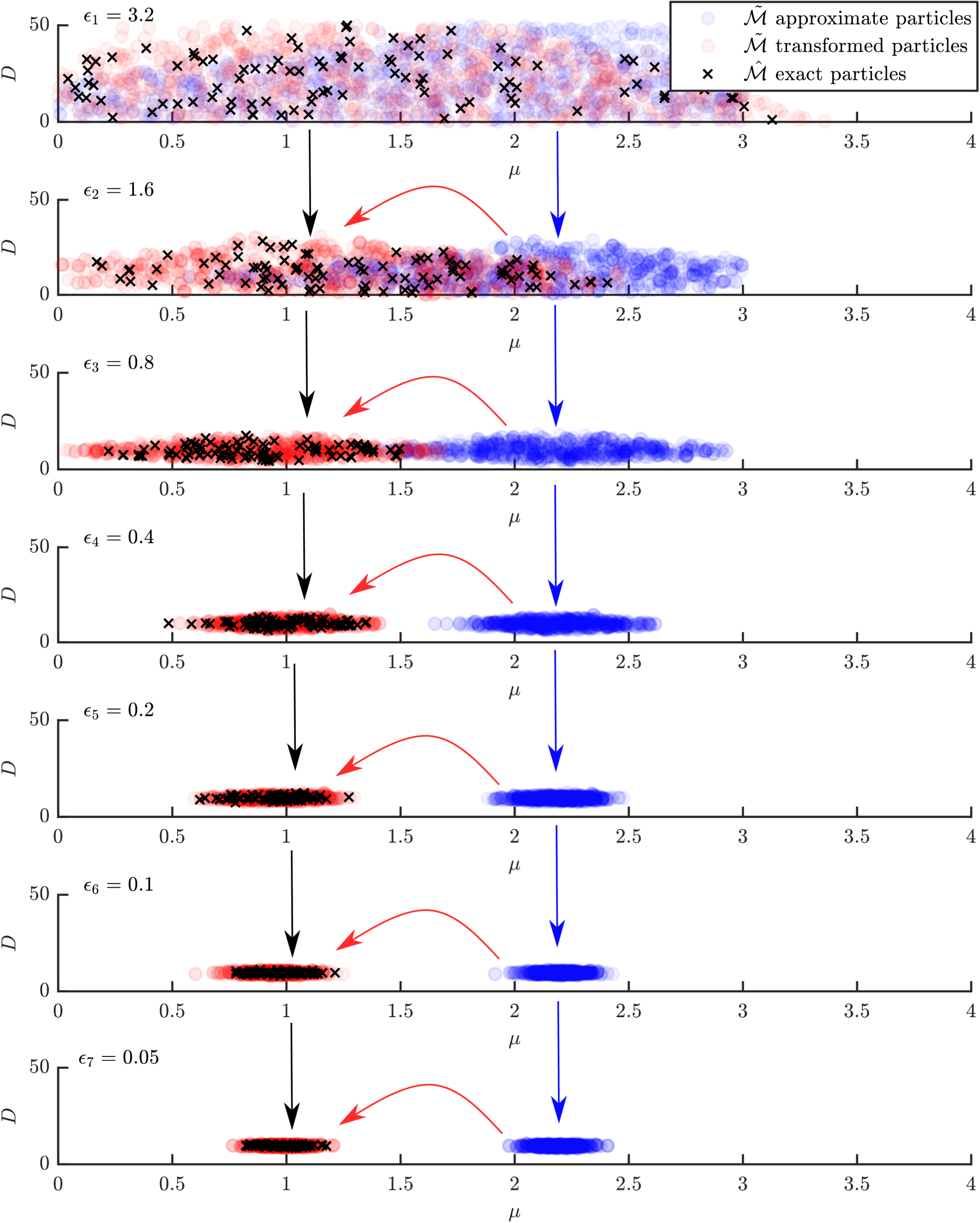
Following the main manuscript, we use Euler-Maruyama simulations Maruyama (1955) with time discretisation (Equation (13) ) for the exact model, and the stationary distribution of the Ornstein-Uhlenbeck process (Equation (14)) for the approximate model. Similarly, the main manuscript is followed for the data which is generated with , , , , , and . To better visually demonstrate MM-SMC-ABC, we infer the joint distribution of where using MM-ABC-SMC (Algorithm 3 in main manuscript) with particles, tuning parameter , and ABC threshold sequence for with .
Figure B.1 demonstrates the movement of approximate particles (blue dots), that are transformed (red dots) using exact particles (black crosses) according to Equation (10) from the main manuscript. For this example, the speedup factor is approximately .
Appendix C Derivation of approximate continuum-limit description
Here we derive the approximate continuum-limit description for our hexagonal lattice based discrete random walk model with generalized crowding function . We follow the method of Simpson et al., Simpson et al. (2010) and Jin et al., Jin et al. (2016).
Our main modification is dealing with a potentially negative crowding function. To deal with this case, we define two auxiliary functions,
| (C.1) |
Note that , as this is important later.
We assume a mean-field, that is, for any two lattice sites, , then their occupancy probabilities are independent, which results in the property,
. Using this property, we denote and write the conservation of probability equation that describes the change in occupancy probability of a site over a single time step,
| (C.2) | ||||
where ,
| (C.3) |
and
| (C.4) |
The conservation of probability equation (Equation C.2) deserves some interpretation. The first term is the probability that site is unoccupied at time and becomes occupied at time due to a successful motility event that moves an agent from an occupied neighboring site into . The second term is the probability that site is occupied at time and becomes unoccupied at time due to a successful motility event that moves the agent away to a neighboring site. The third term is the probability that site is unoccupied at time and becomes occupied at time due to a successful proliferation event from an occupied neighboring site. The final term is the probability that the site is occupied at time and becomes unoccupied at time due to .
For a hexagonal lattice site, , we have six immediate neighboring lattice sites, , , ,
, , and
. The positions of these neighbors are shown in the schematic in Figure C.1.

, , and
.
We obtain an expression for at each of the six neighboring lattice points by associating with a continuous function and performing a Taylor expansion about the point . The result is,
| (C.5) | ||||
Therefore, we obtain an expression for ,
| (C.6) |
This expression is required for the first, second, and fourth terms in the conservation equation (Equation (C.2)).
To deal with the third term in Equation (C.2) we require an expression for
, . By combining Equation (C.5) and Equation (C.6) we obtain
| (C.7) | ||||
Each expression in Equation (C.7) is of the form , where
. This allows us to consider the Taylor expansion of about the density , that is,
| (C.8) |
Using Equation (C.8), we can obtain an expression for the summation within the third term of the conservation equation (Equation (C.2)), that is,
| (C.9) |
After substitution of Equation (C.7) into Equation (C.9) and some tedious algebra we arrive at
| (C.10) |
Finally, we substitute Equation (C.6) and Equation (C.10) into Equation (C.2) to obtain
| (C.11) |
Here we have used the notation , and . After rearranging Equation (C.11), we obtain
| (C.12) |
where
Note that and, by Equation (C.1), that
. Then Equation (C.12) becomes
After dividing by the time interval, , and choosing and , then we have the following limits,
Therefore, we arrive at the continuum-limit approximation
Appendix D Forward problem simulation
This section presents standard computational methods that are applied to forwards problems of the models we consider in this work.
D.1 Stochastic simulation of the discrete model
In the work of Jin et al. Jin et al. (2016), they consider crowding functions with . This is not quite sufficient to enable a crowding function with a carrying capacity since motility events will cause the carrying capacity to be violated. Therefore, we take . If then the site is removed from the set of occupied sites at time , denoted by , with probability . Given these definitions, the lattice-based random walk proceeds according to Algorithm D.1.
D.2 Numerical solutions of continuum-limit differential equations
In our case, the approximate model is a deterministic continuum equation that is either a nonlinear ODE or PDE. In both cases we apply numerical schemes that automatically adapt the time step size to control the truncation error.
D.2.1 ODE numerical solutions
The Runge-Kutta-Fehlberg fourth-order-fifth-order method (RKF45) Fehlberg (1969) is a numerical scheme in the Runge-Kutta family of methods to approximate the solution of a nonlinear ODE of the form,
where is a function that satisfies certain regularity conditions and the initial condition, .
Given the approximate solution, , an embedded pair of Runge-Kutta methods, specifically a fourth and fifth order pair, are used to advanced the solution to and estimate the truncation error that can be used to adaptively adjust to ensure the error is always within some specified tolerance .
The fourth and fifth order estimates are, respectively,
| (D.1) |
and
| (D.2) |
where
Note that the truncation error can be estimated by . After each evaluation of Equation (D.1) and Equation (D.2), a new step size is determined by , where . If , then the solution is accepted and the new is used for the next iteration. Alternatively, if then the solution is rejected and a new attempt is made using the new time step. This process is repeated until the solution advances to some desired time point . For more details and analysis of this method, see Iserles Iserles (2008).
D.2.2 PDE numerical solutions
In this work, we consider numerical solutions to PDEs of the form
| (D.3) |
with initial conditions
and Neumann boundary conditions
Given the approximate solution, for , then we apply a first order backward Euler discretization in time and first order central differences in space to yield
| (D.4) | ||||
where . The solution is stepped forward in time using fixed point iterations that are initialized by a first order forward Euler estimate.
The truncation error is estimated by
After solving the nonlinear system (Equation (D.4)) using fixed point iteration, a new step size is determined by , where and is the truncation error tolerance Simpson et al. (2007); Sloan and Abbo (1999). If , then the solution is accepted and the new is used for the next time step. Alternatively, if then the solution is rejected and a new attempt is made using the new time step. This process is repeated until the solution advances to some desired time point .
Appendix E Additional results
We provide the multivariate posteriors for the results provided in the main text. In both Figure E.1 and Figure E.2 the contours of the posterior bivariate marginals generated, at a significant reduction in computational cost, both the PC-SMC-ABC and MM-SMC-ABC methods align very well with contours of the posterior bivariate marginals SMC-ABC using the expensive discrete model alone, however, the is a clear bias in the contours posterior bivariate marginals generated with SMC-ABC using the continuum-limit approximation alone.
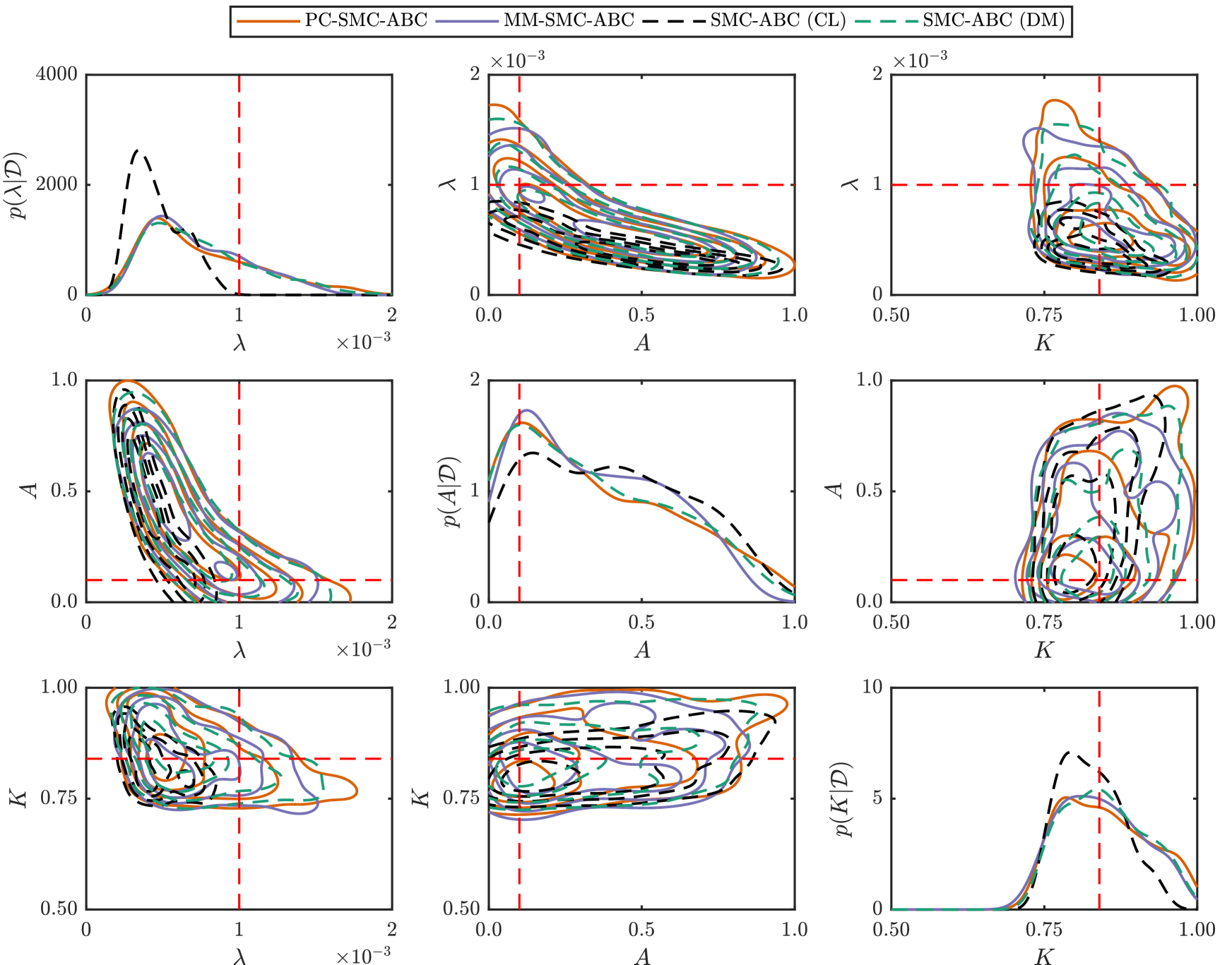
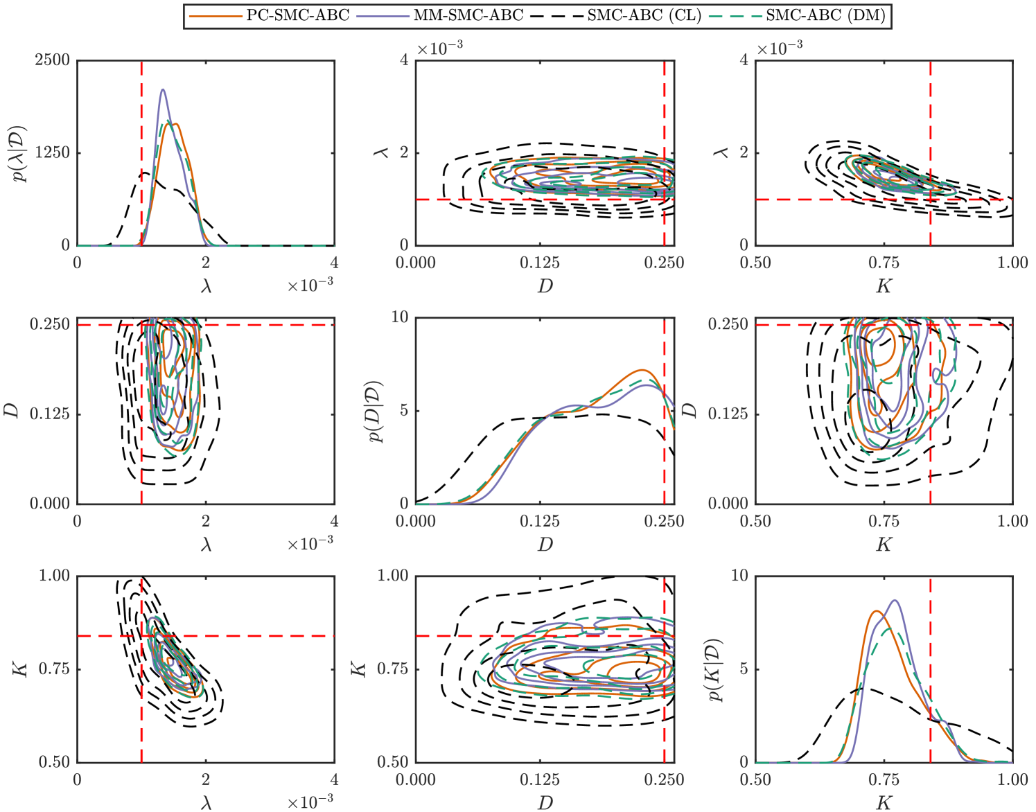
Appendix F Effect of motility rate on continuum-limit approximation
Here we demonstrate the ability (or lack thereof) of the continuum-limit approximation to capture the average behavior of the discrete model for the two examples considered in the main manuscript: the weak Allee model; and the scratch assay model. Figure F.1 plots the solutions to the continuum-limit differential equation against realizations of the discrete model for both motile, , and non-motile, , agents.
In the case of the weak Allee model (Figure F.1(A)), the continuum limit does not match the average behavior in either case, though it does perform better when than when . The remaining discrepancy when is can be related to the ratio and to the effect of the neighborhood radius, (see Jin et al. Jin et al. (2016) for further explanation). Decreasing and increasing will correct this discrepancy. The scratch assay continuum limit captures the average behavior of the discrete model very well when (Figure F.1(B)), but does not capture the scratch closing behavior of the discrete model when (Figure F.1(C)).