Rapid heuristic projection on simplicial cones ^††thanks: 1991 A M S Subject Classification. Primary 90C33; Secondary 15A48, Key words and phrases. Metric projection on simplicial cones

Projection on polyhedral cones is one of the important problems applied optimization is confronted with. Many applied numerical optimization methods uses projection on polyhedral cones as the main tool.

In most of them, projection is part of an iterative process which involve its repeated application (see e. g. problems of image reconstruction [1], nonlinear complementarity [4, 9], etc.). Hence, it is important to get fast projection algorithms.

The main streems of the current methods in use rely on the classical von Neumann algorithm (see e.g. the Dykstra algorithm [3, 2, 10]), but they are rather expensive for a numerical handling (see the numerical results in [7] and the remark preceding section 6.3 in [5]).

Finite methods of projections are of combinatorial nature which reduces their applicability to low dimensional ambient spaces.

Recently we have given a simple projection method exposed in note [8] for projecting on so called isotone projection cones. Isotone projection cones are special simplicial cones, and due to their good properties we can project on them in $n$ steps, where $n$ is the dimension of the ambient space. In the first part of that note we have explained our approach by considering the problem of projection on simplicial cones by giving an exact method based on duality. This method has combinatorial character and therefore it is inefficient. More recently we observed that a heuristic method based on the same ideas gives surprisingly good results. This note describes the theoretical foundation of the heuristic method and draws conclusions based on millions of numerical experiments.

Projection on polyhedral cones is a problem of high impact on scientific community.¹¹1see the popularity of the Wikimization page Projection on Polyhedral Cone at http://www.convexoptimization.com/wikimization/index.php/Special:Popularpages.

Let $\mathbb{R}^{n}$ be an $n$-dimensional Euclidean space endowed with a Cartesian reference system. We assume that each point of $\mathbb{R}^{n}$ is a column vector.

We shall use the term cone in the sense of closed convex cone. That is, the nonempty closed subset $K\subset\mathbb{R}^{n}$ in our terminology is a cone, if $K+K\subset K$, and $tK\subset K$ whenever $t\in\mathbb{R},\;t\geq 0$.

Let $m\leq n$ and $\mathbf{e}_{1},\dots,\mathbf{e}_{m}$ be $m$ elements in $\mathbb{R}^{n}$. Denote

the cone engendered by $\mathbf{e}_{1},\dots,\mathbf{e}_{m}$. Then,

where $\mathbf{E}=(\mathbf{e}_{1},\dots,\mathbf{e}_{m})$ is the matrix with columns $\mathbf{e}_{1},\dots,\mathbf{e}_{m}$ and $\mathbb{R}^{m}_{+}$ is the non-negative orthant in $\mathbb{R}^{m}$.

Suppose that $\mathbf{e}_{1},\dots,\mathbf{e}_{n}\in\mathbb{R}^{n}$ are linearly independent elements. Then, the cone

with $\mathbf{E}$ the matrix from (1) for $m=n$, is called simplicial cone. Denote $N=\{1,2,\dots,n\}$.

The polar of $K$ is the set

$K^{*}=-K^{\circ}$ is called the dual of $K$. $K$ is called subdual, if $K\subset K^{*}$. This is equivalent to the condition $\mathbf{e}_{\ell}^{\top}\mathbf{e}_{k}\geq 0,\,\ell,k\in N.$

Proof. Let $\mathbf{y}=\sum_{j=1}^{n}\mu^{j}\mathbf{u}_{j}$ and $\mathbf{z}=\sum_{i=1}^{n}\alpha^{i}\mathbf{e}_{i}$ for any non-negative real numbers $\alpha^{i}$ and $\mu^{j}$. The inner produce of $\mathbf{y}$ and $\mathbf{z}$ is non-positive because

But $\mathbf{y}$ is an arbitrary element of the right hand side of (4) and $\mathbf{z}$ is an arbitrary element of $K$, thus we can conclude that the righ hand side of (4) is a subset of $K^{\circ}$.

The vectors $\mathbf{u}_{1},\dots,\mathbf{u}_{n}$ are linearly independent. (This can be verified by assuming the contrary, and by multiplying the subsequent relation by $\mathbf{e}_{j}$ to get a contradiction.) Hence for $\mathbf{y}\in K^{\circ}$ we have the representation

By (3),

so $\beta^{k}\geq 0$ which prove that $\mathbf{y}$ is an element of the right hand side of (4). Thus we can conclude that $K^{\circ}$ is a subset of the right hand side of (4). $\Box$

The formula (5) of Lemma 1 is equivalent to the formula (380) of [1].

Proof. Assume that

for some reals $\alpha^{i}$ and $\beta^{j}.$ By the mutual orthogonality of the vectors $\mathbf{e}_{i},i\in I$ and $\mathbf{u}_{j},j\in I^{c}$ it follows, by multiplication of the relation (6) with $\sum_{i\in I}\alpha^{i}\mathbf{e}_{i}^{\top}$ and respectively with $\sum_{j\in I^{c}}\beta^{j}\mathbf{u}_{j}^{\top}$, that

and

Hence, $\alpha^{i}=\beta^{j}=0$ must hold. $\Box$

The cone $K_{0}\subset K$ is called a face of $K$ if from $\mathbf{x}\in K_{0},\mathbf{y}\in K$ and $\mathbf{x}-\mathbf{y}\in K$ it follows that $\mathbf{y}\in K_{0}.$ The face $K_{0}$ is called a proper face of $K$, if $K_{0}\not=K.$

Proof.

The relation in (7) follows from the definition of the vectors $\mathbf{u}_{j}$ in Lemma 1, while the assertion on the dimension of $F_{I}$ is obvious.

Suppose that $\mathbf{x}\in F_{I}$ and $\mathbf{y}\in K$ with $\mathbf{y}\leq\mathbf{x}$.

Then $(\mathbf{x}-\mathbf{y})^{\top}\mathbf{u}_{j}=-\mathbf{y}^{\top}\mathbf{u}_{j}\leq 0$, $\forall j\in I^{c}$ and $\mathbf{y}^{\top}\mathbf{u}_{j}\leq 0,\;\forall j\in N$, because $\mathbf{y}\in K$. Thus $\mathbf{y}^{\top}\mathbf{u}_{j}=0,\;\forall j\in I^{c}$, hence $y\in F_{I},$ showing that $F_{I}$ is a face.

Suppose that $\mathbf{x}\in F$ for $F$ an arbitrary proper face of $K$. Since $\mathbf{x}\in K$, by the definition of the vectors $\mathbf{u}_{j},$ $\mathbf{x}^{\top}\mathbf{u}_{j}\leq 0$ for $j\in N.$

If $\mathbf{x}^{\top}\mathbf{u}_{j}<0,\;\forall j\in N$, then there exists a positive scalar $t$ with $(\mathbf{x}-t\mathbf{y})^{\top}\mathbf{u}_{j}\leq 0,\;\forall j\in N$. Hence, $\mathbf{x}-t\mathbf{y}\in K$ and thus $t\mathbf{y}\leq\mathbf{x}$. But then $t\mathbf{y}\in F$ and since $F$ is a cone, $\mathbf{y}\in F$. This means that $K\subset F$, that is, $F$ cannot be a proper face.

We have to show that $F$ has a representation like (7). By the above reasoning, for each $\mathbf{x}\in F$ there exist some index $i\in N$ with with $\mathbf{x}^{\top}\mathbf{u}_{i}=0.$

If $F=\{\mathbf{0}\}$ we have the representation (7) with $I=\emptyset.$

If $F\not=\{\mathbf{0}\}$, take $\mathbf{x}$ in the relative interior of $F$ and let $I$ be the complement in $N$ of the maximal set of indices $j$ with $\mathbf{x}^{\top}\mathbf{u}_{j}=0.$ ($I$ must be a nonempty, proper subset of $N$ since $\mathbf{x}\not=\mathbf{0}.$)

Take $\mathbf{y}\in F$ arbitrarily. By the definition of $\mathbf{x}$, $\mathbf{x}-t\mathbf{y}\in F$ for some sufficiently small $t>0$. Hence,

By $\mathbf{y}\in F\subset K$ we also have $\mathbf{y}^{\top}\mathbf{u}_{i}\leq 0,\;\forall i\in N.$ If $\mathbf{y}^{\top}\mathbf{u}_{j}<0$ for some $j\in I^{c}$, then (8) would imply

which is a contradiction. Hence, we must have $\mathbf{y}^{\top}\mathbf{u}_{j}=0,\;\forall j\in I^{c}$; and accordingly

Suppose that $\mathbf{y}\in K$ and $\mathbf{y}^{\top}\mathbf{u}_{j}=0,\;\forall j\in I^{c}$. From definition we have $\mathbf{x}^{\top}\mathbf{u}_{i}<0$ for each $i\in I$, whereby for a sufficiently large $t>0$,

Hence, $t\mathbf{x}-\mathbf{y}$ is in the polar of $K^{\circ}$, which by Farkas’ lemma is $K$ (This follows in fact, in our case, also by the symmetry of the vectors $\mathbf{e}_{i}$ and $\mathbf{u}_{j}$ in the formulae of Lemma 1.) Thus $\mathbf{0}\leq\mathbf{y}\leq t\mathbf{x}$, whereby $\mathbf{0}\leq(1/t)\mathbf{y}\leq\mathbf{x}.$ Since $F$ is a face of $K$, we have $(1/t)\mathbf{y}\in F$ and since it is also a cone, $\mathbf{y}\in F.$ This proves the converse of the inclusion in (9) and completes the proof.

$\Box$

Thus a maximal proper face of $K$ is of the form

hence it is also called the face of $K$ orthogonal to $\mathbf{u}_{i_{0}}$. Similarly, we have a maximal proper face of $K^{\circ}$ orthogonal to some $\mathbf{e}_{j_{0}}$.

An equivalent result to the one presented in Lemma 2 is given by the Cone Table 1 on page 179 of [1].

Thus a maximal proper face of $K$ is of the form

hence it is also called the face of $K$ orthogonal to $\mathbf{u}_{i_{0}}$. Similarly, we have a maximal proper face of $K^{\circ}$ orthogonal to some $\mathbf{e}_{j_{0}}$.

Let $F=\operatorname{cone}\{\mathbf{e}_{i}:\;i\in I\}$ and $F^{\perp}=\operatorname{cone}\{\mathbf{u}_{j}:\;j\in I^{c}\}.$ Then, from the above results it follows that

and

The faces $F\subset K$ and $F^{\perp}\subset K^{\circ}$ of the above form are called a pair of orthogonal faces where $F^{\perp}$ is called the orthogonal face of $F$ and $F$ is called the orthogonal face of $F^{\perp}$.

For an arbitrary $\mathbf{u}\in\mathbb{R}^{n}$ denote $\|\mathbf{u}\|=\sqrt{\mathbf{u}^{\top}\mathbf{u}}$. Let $K\in\mathbb{R}^{n}$ be an arbitrary cone and $K^{\circ}$ its polar, and $C\subset\mathbb{R}^{n}$ an arbitrary closed convex set. Recall that the projection mapping $\mathbf{P}_{C}:H\to H$ on $C$ is well defined by $\mathbf{P}_{C}\mathbf{x}\in C$ and

Then, Moreau’s decomposition theorem asserts:

Suppose now, that $K$ is a simplicial cone in $\mathbb{R}^{n}$. We shall use the representation (2) for $K$ and the representation (4) for $K^{\circ}$. Hence,

where $\delta^{i}_{j}$ the Kronecker symbol. As a direct implication of Moreau’s decomposition theorem and the constructions in the preceding section we have:

Proof. The first assertion is the consequence of Corollary 1.

The projections $\mathbf{P}_{K}\mathbf{x}$ and $\mathbf{P}_{K^{\circ}}\mathbf{x}$ as elements of $K$ and $K^{\circ}$, respectively can be represented as

and

To prove existence, let $I^{c}=\{j\in N:\beta^{j}>0\}$ and let $I$ be the complement of $I^{c}$ in the set $N$ of indices. For an arbitrary element $\mathbf{z}\in\mathbb{R}^{n}$, denote $\mathbf{P}_{K}^{\top}\mathbf{z}=(\mathbf{P}_{K}\mathbf{z})^{\top}$. If $\alpha^{j}>0$ would hold in (14), for some $j\in I^{c}$, then by Lemma 1 it would follow that $\mathbf{P}_{K}^{\top}\mathbf{x}\cdot\mathbf{P}_{K^{\circ}}\mathbf{x}<0,$ which contradicts the theorem of Moreau. Hence, (13) can be written in the form (11) and (14) can be written in the form (12). Therefore, Theorem 1 implies

where $\alpha^{i}\geq 0$, $\forall i\in I$ and $\beta^{j}>0$, $\forall j\in I^{c}$.

To prove uniqueness, suppose that in the representation (10) of $\mathbf{x}$ we have $\alpha^{i}\geq 0,\;\beta^{i}=0$ for $i\in I$ and $\beta^{j}>0,\;\alpha^{j}=0$ for $j\in I^{c}$, where $I$ is a subset of $N$, and $I^{c}$ is the complement of $I$ in $N$ (the cases $I=\emptyset$ and $I=N$ are not excluded). Then representations (11) and (12) follow from Theorem 1 by using the mutual orthogonality of the vectors $\mathbf{e}_{i},\;i\in I$ and $\mathbf{u}_{j},\;j\in I^{c}$. From (11) and the uniqueness of the projection $\mathbf{P}_{K}\mathbf{x}$ it follows that $I$ is unique.

$\Box$

From this theorem it follows that a given simplicial cone $K\subset\mathbb{R}^{n}$ determines a partition of the space $\mathbb{R}^{n}$ in $2^{n}$ cones in the sense that

and for two different sets $I$ of indices the respective cones do not contain common interior points. The cones in the above union are exactly the sums of orthogonal faces.

This theorem suggests the following algorithm for finding the projection $\mathbf{P}_{K}\mathbf{x}$:

Step 1. For the subset $I\subset N$ we solve the following linear system in $\alpha^{i}$

Step 2. Then, we select from the family of all subsets in $N$ the subfamily $\Delta$ of subsets $I$ for which the system possesses non-negative solutions.

Step 3. For each $I\in\Delta$ we solve the linear system in $\beta^{j}$

By Theorem 2 among these systems there exists exactly one with non-negative solutions. By this theorem, for corresponding $I$ and for the solution of the system (15), we must have

This algorithm requires that we solve $2^{n}$ linear systems of at most $n$ equations in Step 1 (15) and another $2^{|\Delta|}$ systems in Step 2 (16). (Observe that all these systems are given by Gram matrices, hence they have unique solutions.) Perhaps this great number of systems can be substantially reduced, but it still remains considerable.

Regardless the inconveniences of the above presented exact method, which follow from its combinatorial character, it suggests an interesting heuristic algorithm. To explain its intuitive background we consider again the simplicial cone

and its polar

given by Lemma 1.

Take an arbitrary $\mathbf{x}\in\mathbb{R}^{n}$. We are seeking the projection $\mathbf{P}_{K}x.$

If $\mathbf{e}_{i}^{\top}\mathbf{x}\leq 0,\;\forall\;i\in N$, then $\mathbf{x}\in K^{\circ}=\ker\mathbf{P}_{K}$, hence $\mathbf{P}_{K}\mathbf{x}=0.$

If $\mathbf{u}_{j}^{\top}\mathbf{x}\leq 0,\;\forall\;j\in N$, then $\mathbf{x}\in K$, and hence $\mathbf{P}_{K}\mathbf{x}=\mathbf{x}$.

We can assume that $\mathbf{x}\notin K\cup K^{\circ}$. Hence, $\mathbf{x}$ projects in a proper face of $K$ and in a proper face of $K^{\circ}.$

Take an arbitrary family $I\subset N$ of indices. Then, the vectors

entgender by Corollary 1 a reference system in $\mathbb{R}^{n}$. Then,

with some $\alpha^{i},\;\beta^{j}\in\mathbb{R}.$ (As far as the family $I\subset N$ of indices is given, we can determine the coefficients $\alpha^{i}$ and $\beta^{j}$, according to Theorem 2, by solving the systems (15) and (16).)

If we have $\alpha^{i}\geq 0,\;\beta^{j}\geq 0:\;i\in I,\;j\in I^{c}$, then from Theorem 2 we obtain

and

In this case $\mathbf{x}$ is projected onto face $F=\operatorname{cone}\{\mathbf{e}_{i}:\;i\in I\}$ ortogonally along the subspace engendered by the elements $\{\mathbf{u}_{j}:\;j\in I^{c}\}$, roughly speaking, along the orthogonal face $F^{\perp}$ of $F$.

Suppose that $\beta^{j}<0$ for some $j\in I^{c}$. Then, considering the reference system entgendered by $\mathbf{e}_{i},\;\mathbf{u}_{j},\;i\in I,\;j\in I^{c}$, $\mathbf{x}$ lies in its orthant with negative $j^{th}$ coordinate, that is in the direction of the vector $-\mathbf{u}_{j}$. By construction, $\mathbf{e}_{j}$ and $\mathbf{u}_{j}$ form an obtuse angle. Hence the angle of $\mathbf{e}_{j}$ and $-\mathbf{u}_{j}$ is an acute one. Thus there is a real chance that in a new reference system in which $\mathbf{e}_{j}$ replaces $\mathbf{u}_{j}$, the coordinate of $\mathbf{x}$ with respect to $\mathbf{e}_{j}$ has the same sign as its coordinate with respect to $-\mathbf{u}_{j}$, that is positive (or at least non-negative).

If we have $\alpha^{i}<0$ for some $i\in I$, then by similar reasoning it seems to be advantageous to replace $\mathbf{e}_{i}$ with $\mathbf{u}_{i}$, and so on.

Thus, we arrive to the following step in our algorithm:

Substitute $\mathbf{u}_{j}$ with $\mathbf{e}_{j}$ if $\beta^{j}<0$ and substitute $\mathbf{e}_{i}$ with $\mathbf{u}_{i}$ if $\alpha^{i}<0$ and solve the systems (15) and (16) for the new configuration of indices $I$. We shall call this step an iteration of the heuristic algorithm.

Then, repeat the procedure for the new configuration of $I$ and so on, until we obtain a representation (17) of $\mathbf{x}$ with all the coefficients non-negative.

The heuristic algorithm was programmed in Scilab, an open source platform for numerical computation.²²2http://www.scilab.org/ Experiments were performed on numerical examples for $2,\,3,\,5,\,10,\,15,\,20,\,25,\,30,\,50,\,75,\,100,\,200,\,300,\,500$ dimensional cones. The algorithm was performed on $100000$ random examples for each of the problem sizes $2,\dots,\,100$. Statistical analysis on a subset of $10000$ examples from the set of $100000$ examples for size $100$ indicates no significant difference in overall results and performance, therefore we subsequenlty reduced the number of experiments on larger problem sizes. $10000$ random examples were used for sizes $200$ and $300$ and $1000$ examples for size $500$, as the time needed by the algorithm increases with size.

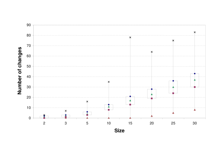
Table 1 shows the experimental results. For each problem size, the averages of all runs are shown, together with a confidence interval at confidence level $95\%$ where appropriate.³³3Any difference less than $\pm 0.5$ for integers and $\pm 0.1$ for percentages, respectively, is not shown, as deemed irrelevant for the analysis. The Changes column indicates the total number of swaps $\mathbf{u}_{j}$ for $\mathbf{e}_{j}$ and $\mathbf{e}_{j}$ for $\mathbf{u}_{j}$, respectively, before reaching the solution. The Iterations column indicates the number of iterations (as defined in Section 4) the algorithm performed before reaching a solution. The Iterations with increases column shows the percentage of iterations where the number of changes increased from the previous iteration. We noticed that in the majority of iterations the number of changes decreased, which led to the quick convergence of the algorithm in the vast majority of cases. In all examples the starting point for the search was the $\mathbf{e}_{1},\dots,\,\mathbf{e}_{n}$ base. The final column shows the percentage of problems where the algorithm was aborted due to going in a loop by allocating in some iteration a set of $\mathbf{e}_{j}$s and $\mathbf{u}_{j}$s that were encountered in a previous iteration. The percentage of loops was exponentially decreasing as the size increased and we did not observe any loops in any experiments on problem sizes of $30$ or above. Overall, loops were observed in $0.1\%$ of the experiments, so the heuristic algorithm was successful $99.9\%$ of the time. A solution that we see for solving the problems that lead to a loop is to restart the algorithm from a different initial set of $\mathbf{e}_{j}$s and $\mathbf{u}_{j}$s. The problems ending in a loop were excluded from the detailed analysis that follows.

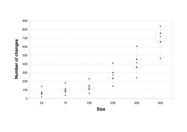
More detailed analysis of the three main performance indicators of changes, iterations and iterations with increases was performed using boxplots as shown in Figures 1, 2 and 3. Although the total number of changes performed increases linearly with problem size (at a rate of less than $2\times n$, even if considering maximum numer of changes), this does not affect the performance substantially (see Figure 1, where the results were split into two parts for a clearer view).

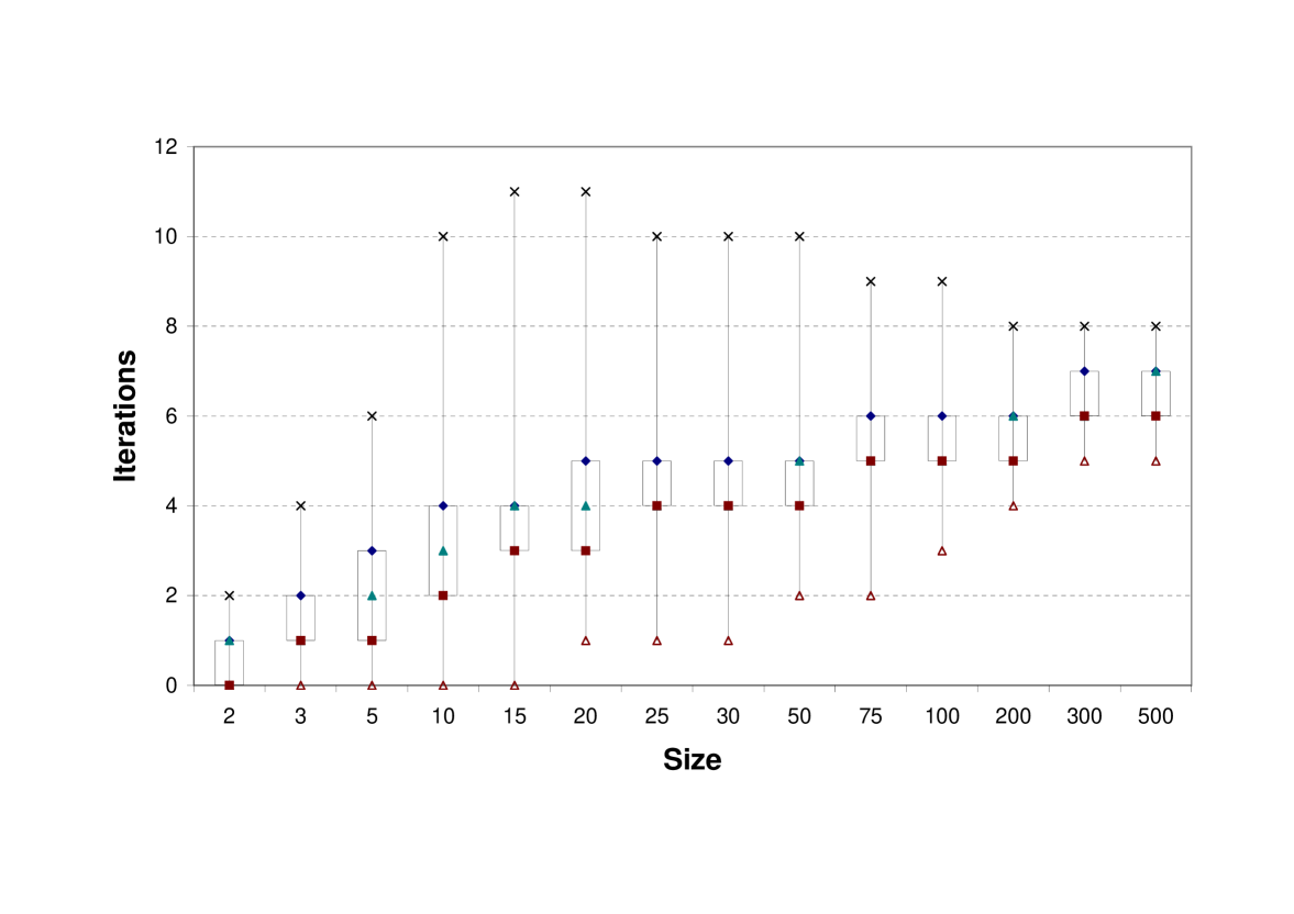
The number of iterations is the crucial indicator of performance. As shown in Figure 2 the number of iterations reaches at most $11$ (for sizes $15$ and $20$), but in $75\%$ of cases has a value of $7$ or below. We ran a few experiments on larger sizes, up to $1750$, and the largest number of iterations we obeserved was $13$. Running experiments on very large problem sizes is problematic due to computer memory limitations and the Scilab built-in solving of linear systems.⁴⁴4 Note that the time needed by one iteration substantially increases with problem size $n$ as one iteration involves solving a linear system with $n$ equations and $n$ variables. The major benefit of this heuristic algorithm is the small number of iterations even for very large number of cone dimensions.

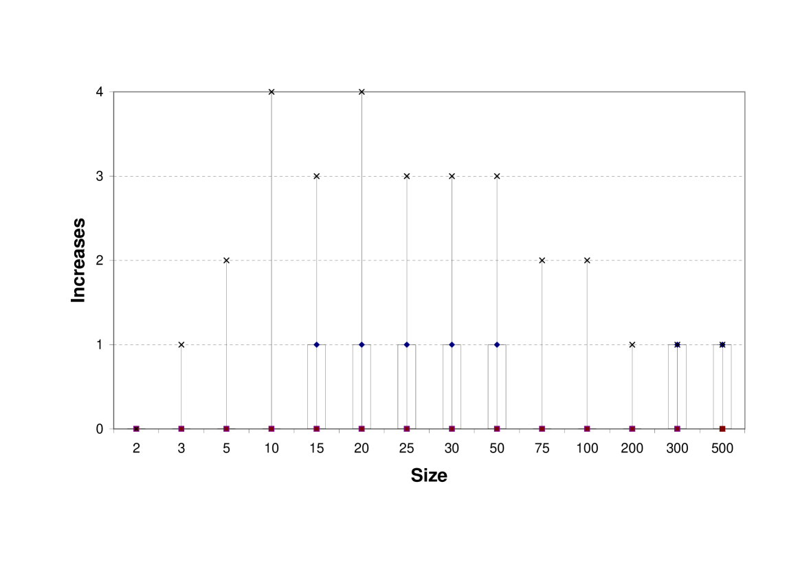
As our heuristic algorithm seems to converge quickly, we wanted to know how frequently it deviates from the optimal path. An optimal path would consist of iterations with decreasing number of changes. Figure 3 shows the boxplots for the number of iterations where an increase in the number of changes took place. The maximum number of such iterations over all experiments is $4$, but $75\%$ of examples involved only one or no such iteration. This provides an explanation for the fast convergence: the algorithm very rarely deviates from the optimal path.

We presented a heuristic method of projection on simplicial cones based on Moreau’s decomposition theorem. The heuristic algorithm presented in this note iteratively finds the projection onto a simplicial cone in a surprisingly small number of steps even for large cone dimensions in $99.9.\%$ of the cases. We attribute the success to the fact that the algorithm rarely deviates from the optimal path, in every iteration it usually has to change less base values than in the previous iteration. We are planning to further extend the algorithm with random restart hoping to achieve $100\%$ success rate.

S. Z. Németh was supported by the Hungarian Research Grant OTKA 60480. The authors are grateful to J. Dattorro for many helpful conversations.

References

- [1] J. Dattorro. Convex Optimization Euclidean Distance Geometry. , 2005, v2009.04.11.
- [2] F. Deutsch and H. Hundal. The rate of convergence of Dykstra’s cyclic projections algorithm: the polyhedral case. Numer. Funct. Anal. Optim., 15(5-6):537–565, 1994.
- [3] R. L. Dykstra. An algorithm for restricted least squares regression. J. Amer. Stat. Assoc., 78(384):273–242, 1983.
- [4] G. Isac and A. B. Németh. Projection methods, isotone projection cones, and the complementarity problem. J. Math. Anal. Appl., 153(1):258–275, 1990.
- [5] T. Ming, T. Guo-Liang, F. Hong-Bin, and Ng. Kai Wang. A fast EM algorithm for quadratic optimization subject to convex constraints. Statist. Sinica, 17(3):945–964, 2007.
- [6] J. J. Moreau. Décomposition orthogonale d’un espace hilbertien selon deux cônes mutuellement polaires. C. R. Acad. Sci., 255:238–240, 1962.
- [7] P. M. Morillas. Dykstra’s algorithm with strategies for projecting onto certain polyhedral cones. Applied Mathematics and Computation, 167(1):635–649, 2005.
- [8] A. B. Németh and S. Z. Németh. How to project onto an isotone projection cone. Linear Algebra Appl., submitted.
- [9] S. Z. Németh. Iterative methods for nonlinear complementarity problems on isotone projection cones. J. Math. Anal. Appl., 350(1):340–347, 2009.
- [10] X. Shusheng. Estimation of the convergence rate of Dykstra’s cyclic projections algorithm in polyhedral case. Acta Math. Appl. Sinica (English Ser.), 16(2):217–220, 2000.