RASPNet: A Benchmark Dataset for Radar Adaptive
Signal Processing Applications
RASPNet: Supplementary Information
Abstract
We present a large-scale dataset for radar adaptive signal processing (RASP) applications to support the development of data-driven models within the adaptive radar community. The dataset, RASPNet, exceeds 16 TB in size and comprises 100 realistic scenarios compiled over a variety of topographies and land types from across the contiguous United States. For each scenario, RASPNet consists of 10,000 clutter realizations from an airborne radar setting, which can be used to benchmark radar and complex-valued learning algorithms. RASPNet intends to fill a prominent gap in the availability of a large-scale, realistic dataset that standardizes the evaluation of adaptive radar processing techniques and complex-valued neural networks. We outline its construction, organization, and several applications, including a transfer learning example to demonstrate how RASPNet can be used for realistic adaptive radar processing scenarios.
1 Introduction
The success of radar technologies over the past century has been characterized by landmark advances in signal processing techniques. In this domain of radar adaptive signal processing (RASP), Space-Time Adaptive Processing (STAP) has been instrumental in achieving order-of-magnitude improvements in detection and localization performance, especially in environments dominated by interference and noise, which has revolutionized modern radar systems (Brennan & Reed, 1973). For decades, STAP has been integral to advancing surveillance, defense, and navigation (Ward, 1995; Li & Stoica, 2008). The foundations of RASP, realized using STAP, lies in the adaptive combination of spatial and temporal processing to optimize radar response to signals (Ward, 1998; Guerci, 2000; Melvin, 2004; Wicks et al., 2006).
Despite the theoretical and practical advancements in RASP, the development, testing, and validation of RASP algorithms remains a significant challenge. This difficulty arises from the complexity of the real-world scenarios in which radar systems operate, which are characterized by dynamic and unpredictable environmental conditions. Theoretical models alone cannot capture the full range of operational scenarios, limiting the effectiveness of RASP algorithms developed in a vacuum (Klemm, 2002; Melvin, 2004).
Paralleling the evolution of adaptive radar, complex-valued neural networks (CVNNs) have emerged as promising tools for enhancing signal processing capabilities (Hirose et al., 2006; Trabelsi et al., 2017; Wu et al., 2023). While CVNNs are well-suited for handling the inherently complex-valued data produced by radar systems, benchmarking CVNNs is limited by a lack of comprehensive datasets with naturally occurring complex-valued features (Mohammadi Asiyabi et al., 2023). Practitioners often convert real-valued datasets to the frequency domain for benchmarking (Trabelsi et al., 2017; Scardapane et al., 2020), which fails to capture the nuanced characteristics of real-world complex-valued data.
The need for large-scale, comprehensive, realistic datasets in the adaptive radar community cannot be overstated. High-quality datasets serve multiple critical functions in the development lifecycle of RASP algorithms. Firstly, they provide a benchmark for evaluating and comparing the performance of algorithms under a wide range of conditions that mirror real-world operational environments. Furthermore, these datasets facilitate the development of data-driven approaches that leverage machine learning and artificial intelligence (Hara et al., 1994; Jiang et al., 2022; Venkatasubramanian et al., 2023). The Knowledge Aided Sensor Signal Processing and Expert Reasoning (KASSPER) dataset represents a seminal effort in this direction (Guerci & Baranoski, 2006), offering a focused repository of radar data that has been significant in advancing the field (Crooks, 2004; Blunt et al., 2006; Stoica et al., 2008; Wang et al., 2009).
In spite of the value provided by existing repositories like KASSPER, the adaptive radar community continues to face data-related challenges. KASSPER, for instance, comprises one radar scenario, which is inadequate for data-driven algorithms. Thus, the primary issue is the absence of a publicly available dataset that encompasses the diversity of scenarios that adaptive radar systems encounter, as existing datasets are either too narrow in scope or restricted in accessibility and utility (Gogineni et al., 2022).
To address these challenges, we present RASPNet, a large-scale, benchmark dataset for radar adaptive signal processing applications. RASPNet comprises a comprehensive set of scenarios from across the United States, compiled over a variety of environmental conditions, topographies, and land types via the RFView® modeling and simulation software. For each scenario, we provide realizations of clutter returns gathered with an airborne radar platform over a kilometer distance. RASPNet has the flexibility to support both traditional RASP algorithms and emerging data-driven approaches, facilitating a concrete benchmark to compare the performance of adaptive radar processing methods, and providing a critical testbed for CVNNs.
The outline of this paper is as follows. In Section 2, we discuss the properties of RASPNet, including the radar parameters used to generate the dataset, the radar scenarios in the dataset, and validate RFView® versus measured data. In Section 3, we describe the organization of RASPNet via the energy distance metric. In Section 4, we delineate two relevant applications of RASPNet for benchmarking target localization accuracy, and for transfer learning in realistic adaptive radar processing scenarios. Finally, in Section 6, we summarize RASPNet and discuss future work. RASPNet is accessible at https://shyamven.github.io/RASPNet.
2 Dataset Properties
We first describe the procedure used to generate the scenarios comprising RASPNet and detail the intuition behind our scenario choices, subject to empirical validation.
2.1 Radar Platform Parameters
To obtain the data for each scenario comprising RASPNet, we make use of the RFView® modeling and simulation tool. This physics-based, RF modeling and simulation platform integrates a global database of terrain and land cover for RF ray tracing simulations. RFView® has been compared with measured datasets from VHF to Ka band (Gogineni et al., 2022). We further validate RFView® versus the MCARM measured dataset (Babu et al., 1996) in Section 2.4.
The scenarios we consider simulate an airborne radar surveying various regions across the United States. For simplicity, the radar was assumed as static during the simulation. The complete list of radar platform parameters is provided in Table 4 of the Supplementary Information.
We position the radar platform at a preset, scenario-specific, latitude and longitude location, utilizing the parameters from Table 4. The radar platform aims km to the southwest and operates in spotlight mode. The clutter return is beamformed for each size receiver sub-array, condensing the array to size . Formally, let denote the set of scenario indices, where is the total number of scenarios within the dataset. We denote as the random variable describing the clutter for scenario . Now, consider , which denotes the clutter return for the th independent realization for scenario . To obtain the clutter dataset for scenario , we obtain i.i.d. realizations to form , where .
2.2 Radar Scenarios
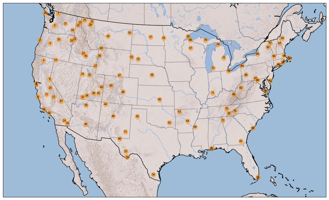
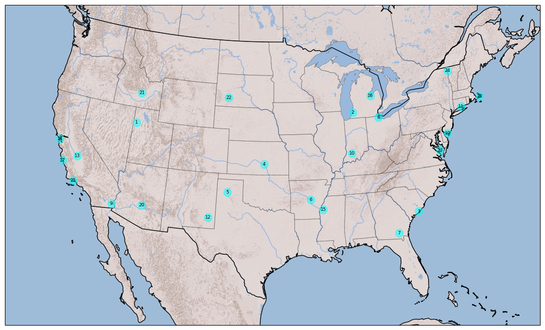
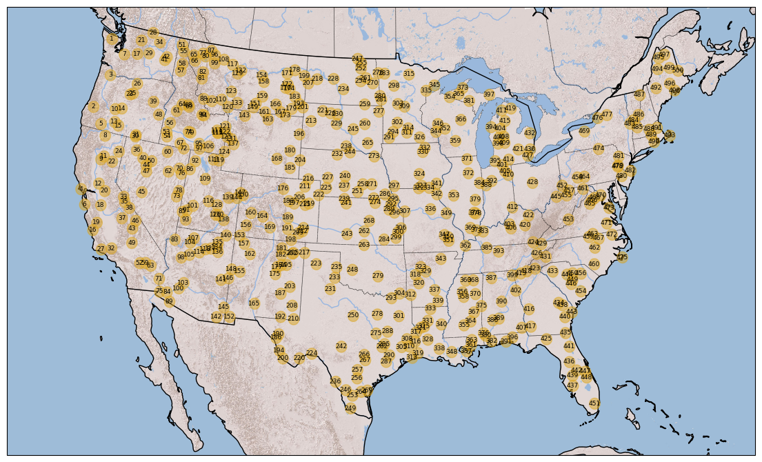
RASPNet comprises hand-picked scenarios from the contiguous United States, where the clutter dataset for each scenario, with , is obtained via the procedure described in Section 2.1. The selection criteria for these scenarios prioritize geographical diversity, focusing on varied landforms and topographies that present distinct challenges for radar systems. The geographic coverage of RASPNet scenarios across the contiguous United States is depicted in Figure 1, wherein the indices, , are ordered from the westernmost to easternmost scenario by default.
To evaluate whether RASPNet encompasses a realistic and extensive feature set, we empirically verify the exemplar nature of our hand-picked scenarios in Section 2.3. Additionally contained within these scenarios are land-to-water transition scenarios, which capture the complexities associated with implementing adaptive radar processing algorithms in coastal regions. The complete tabulation of scenarios comprising RASPNet, along with short descriptions, is provided in Section G of the Supplementary Information.
2.3 Exemplar Scenario Validation
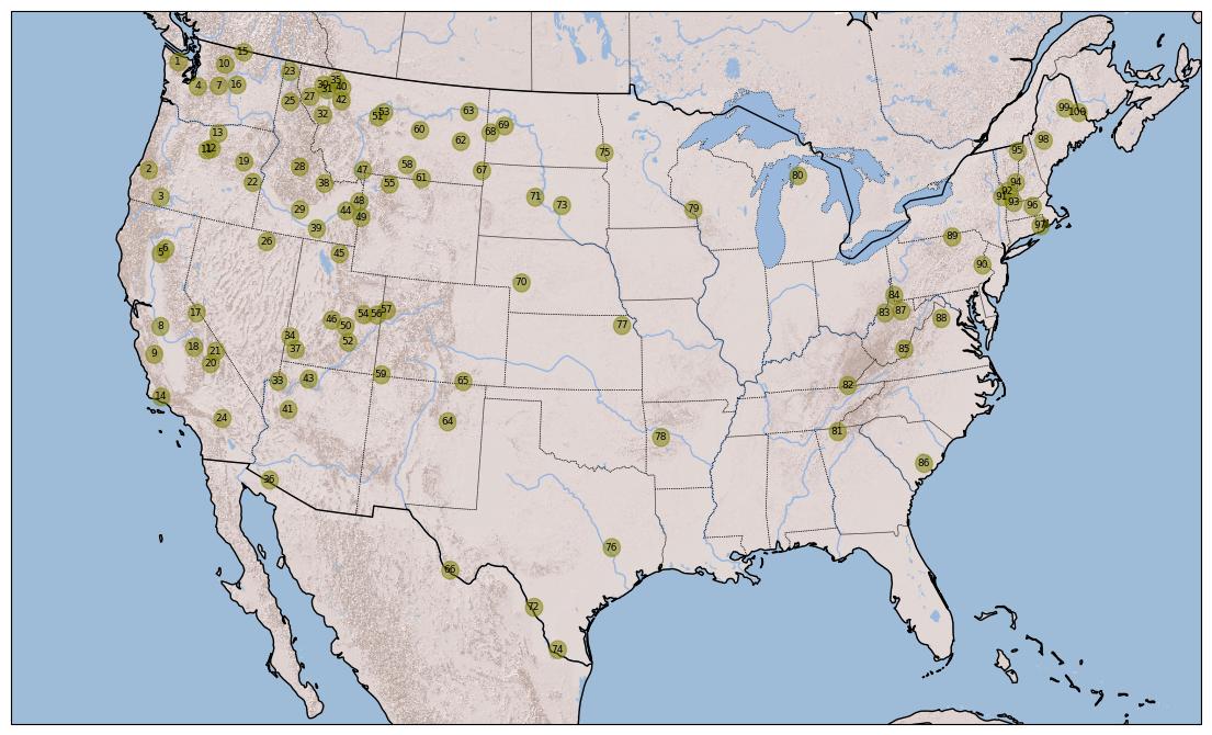
To determine whether our hand-picked scenarios are exemplar, we compare their geographic coverage with that of a collection of scenarios obtained through the Partitioning Around Medoids (PAM) algorithm (Kaufman & Rousseeuw, 1990), from total scenarios uniformly selected at random across the contiguous United States. We denote as the set of indices pertaining to the scenarios, and denote as the set of indices yielded by PAM, where .
To determine using the PAM algorithm, we employ the energy statistic (-statistic) as our distance metric (Székely & Rizzo, 2013). The -statistic quantifies the statistical distance between the distributions of random variables by aggregating pairwise sample distances, capturing differences in their distributional characteristics. Rooted in potential energy principles, the -statistic facilitates robust comparisons of complex, multivariate datasets beyond location or scale. The formal definition of the -statistic for our analysis is provided in Definition 2.1.
Definition 2.1.
Consider clutter random variables , for , wherein we have the clutter datasets , . The -statistic is given by:
| (1) | |||
We now outline the PAM algorithm for our analysis. We first construct the -statistic matrix, , for , where each element, , is precomputed using for every pair . This precomputation step facilitates efficient distance lookups during the PAM algorithm’s execution. Subsequently, over steps, the PAM algorithm iteratively refines a subset of representative scenarios, , through a process of swapping current medoids with non-medoids to minimize the total cost, , where is computed as the sum of distances from each scenario to its nearest medoid, based on the precomputed -statistic matrix, . This procedure is summarized in Algorithm 1. The total scenarios and the representative scenarios from PAM are depicted in Section A of the Appendix.
We observe that the geographic coverage of the hand-picked scenarios in RASPNet closely mirrors the coverage of the representative scenarios determined through PAM. A large concentration of these scenarios are in the Western United States — this region is characterized by a wider variety of terrain types, which introduces greater variability in the distribution of geographic features, leading to a greater concentration of representative scenarios. We also note that the hand-picked scenarios in RASPNet are more dispersed across the contiguous United States by construction, particularly because they encompass identifiable geographical landmarks representing a broad spectrum of environmental conditions. A greater emphasis was also placed on incorporating land-to-water transition zones in the hand-picked scenarios, acknowledging these as inherently more varied scenarios.
2.4 Validation Against Measured Data
To evaluate the realistic nature of the RFView® simulator, we compare it with the MCARM measured dataset, focusing on Flight #5 Acquisition 575 (Babu et al., 1996). The MCARM radar parameters are tabulated in Section B of the Appendix. Let , for , denote the clutter random variables for the MCARM, RFView®, and bald-earth (BE) models, wherein the bald-earth model is a more classical clutter model without terrain heights. For the RFView® and BE models, we generate the clutter datasets and , which we then reshape to obtain . The MCARM Flight #5 Acquisition 575 provides a single clutter realization, , which we reshape to form .
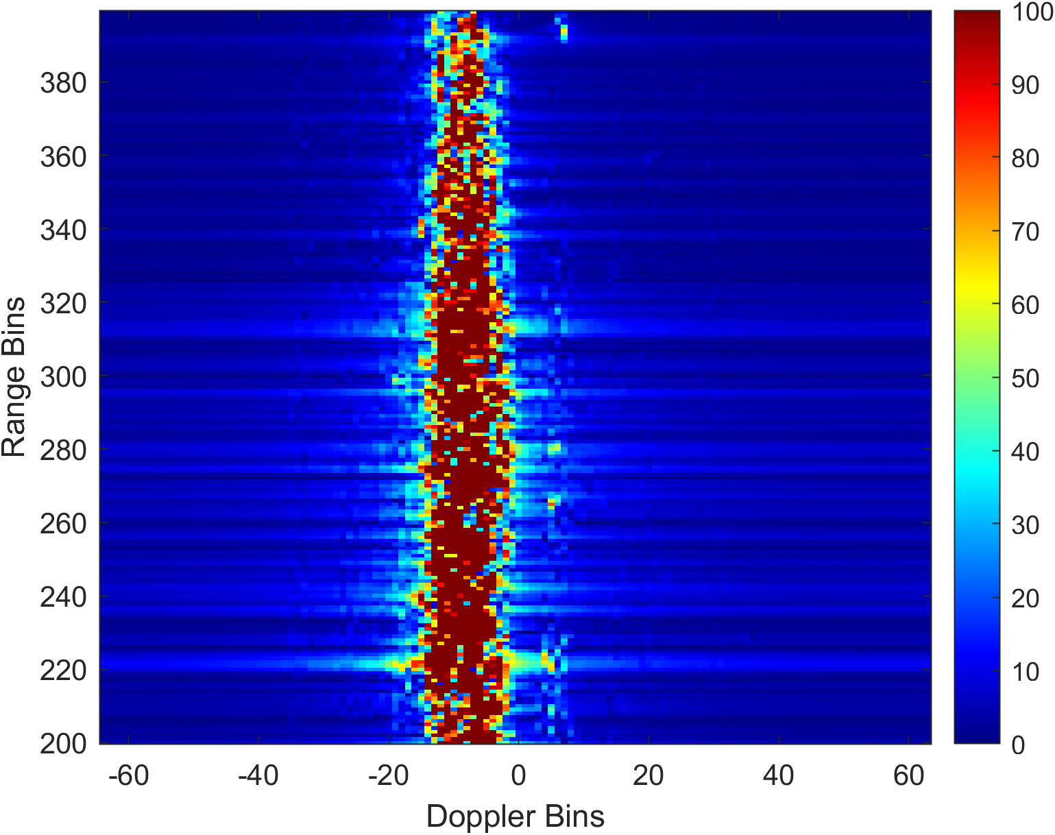
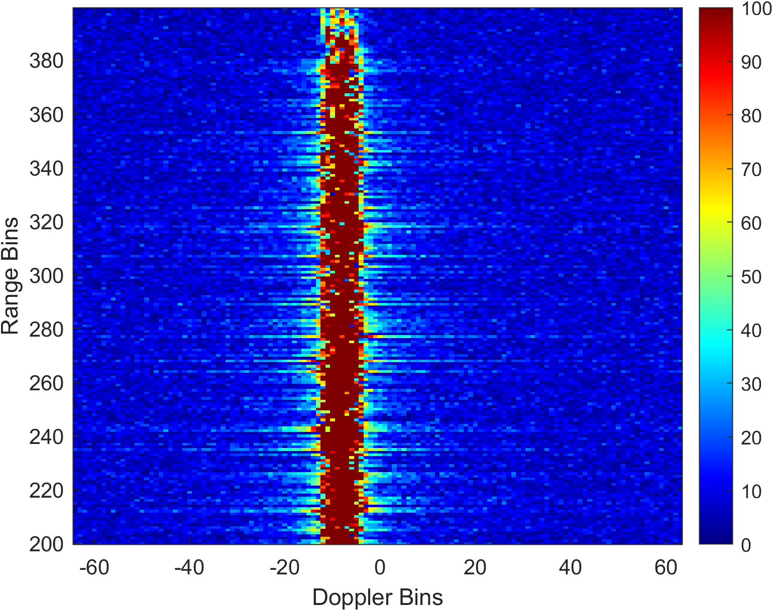
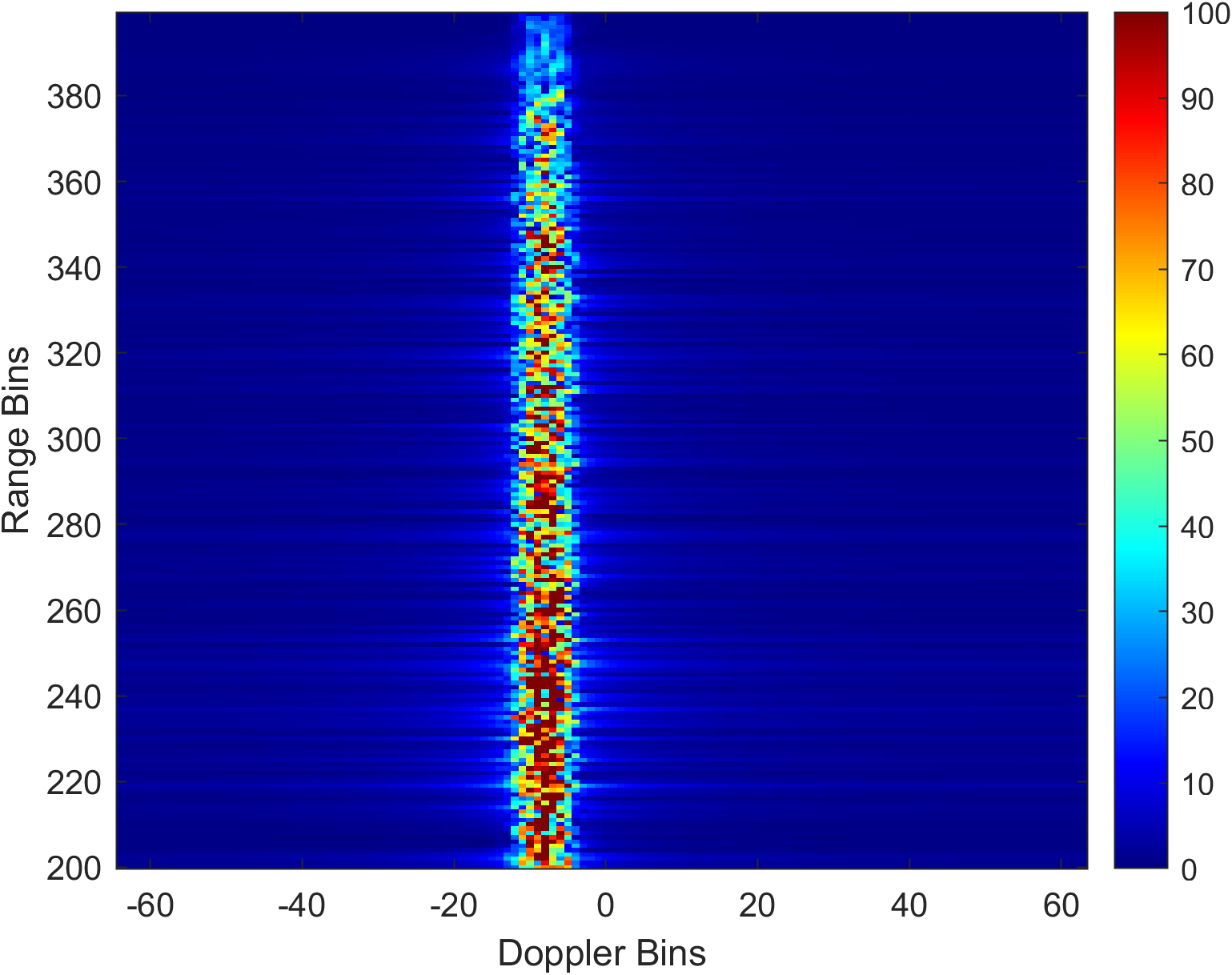
We produce range-Doppler plots for both the RFView® simulated data and the MCARM measured data by performing Doppler processing via the Fast Fourier Transform (FFT), coherently integrating across antenna elements. The range-Doppler plots for the MCARM, RFView®, and BE models are shown in Figure 2. We clearly observe that the RFView-generated data exhibits a higher degree of similarity to the MCARM measured data than the classical BE model.
To validate the similarity between the RFView® simulated data and the MCARM measured data, we perform a modified version of the likelihood-based test from (Johnson & Abramovich, 2010). Let , , and form the MCARM, RFView®, and bald-earth clutter realizations, for the -th Doppler bin and -th range bin. The null hypothesis, , asserts that is from the same distribution as — we repeat this procedure for ). Next, , we compare the likelihood of the MCARM clutter realization to the empirical distribution of likelihoods from the RFView® clutter realizations. We let denote the sample covariance matrix for the RFView case, where the likelihood of the MCARM data given , and the likelihood of the RFView clutter realization given , are given by:
| (2) | ||||
| (3) |
To determine if the real-world data is consistent with the simulated data distribution, we compare to the empirical distribution of . We form the confidence interval from the percentiles of . If falls within this confidence interval, we fail to reject . We compute the total fraction of how often the MCARM likelihood falls in the confidence interval over all Doppler and range bins, denoted :
| (4) | ||||
In the RFView® case (), we obtain for the real part of , for the imaginary part of . In the bald-earth case (), we obtain for both the real and imaginary parts of . This study shows that while RFView® does not offer a complete match with the real-world data, it is more realistic than the bald-earth model. Furthermore, this study suggests that for real-world applications, it is feasible to train networks on RASPNet scenarios, and fine tune them using real-world samples. We explore this further in Section 4.3.
3 Dataset Organization
The organization of RASPNet is guided by the premise of ranking scenarios based on their difficulty for RASP algorithms, which we quantify using the -statistic. We employ this metric to systematically order the scenarios from the most similar to the baseline scenario, defined as index from (the Bonneville Salt Flats), to the least similar, as a proxy for difficulty. This baseline scenario typifies an environment that has minimal variability in elevation and a uniform land type — characteristics that typically simplify adaptive processing tasks. We denote as the sequence of ordered indices, and let be an -dimensional array with elements , where , and is the index of the baseline scenario. Thus, the scenario corresponds to the ‘easiest’ scenario, , in RASPNet. We summarize this ordering procedure in Algorithm 2.
The rationale behind using the -statistic with respect to the Bonneville Salt Flats as a benchmark is its inherent simplicity for RASP algorithms. Scenarios with lower -values relative to this baseline are deemed less challenging, as their clutter characteristics more closely resemble those of an environment with low variability and uniformity, simplifying the radar’s task of distinguishing between targets and clutter. Conversely, scenarios with higher -values are deemed more challenging as they indicate nonuniform environments, requiring advanced radar processing algorithms.
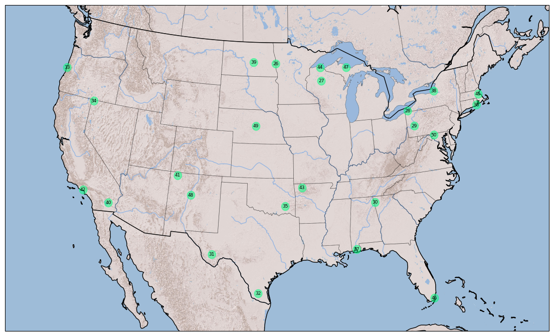
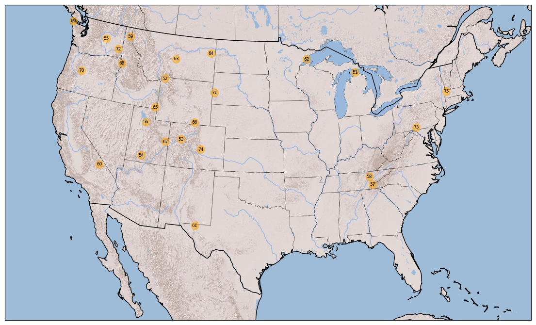
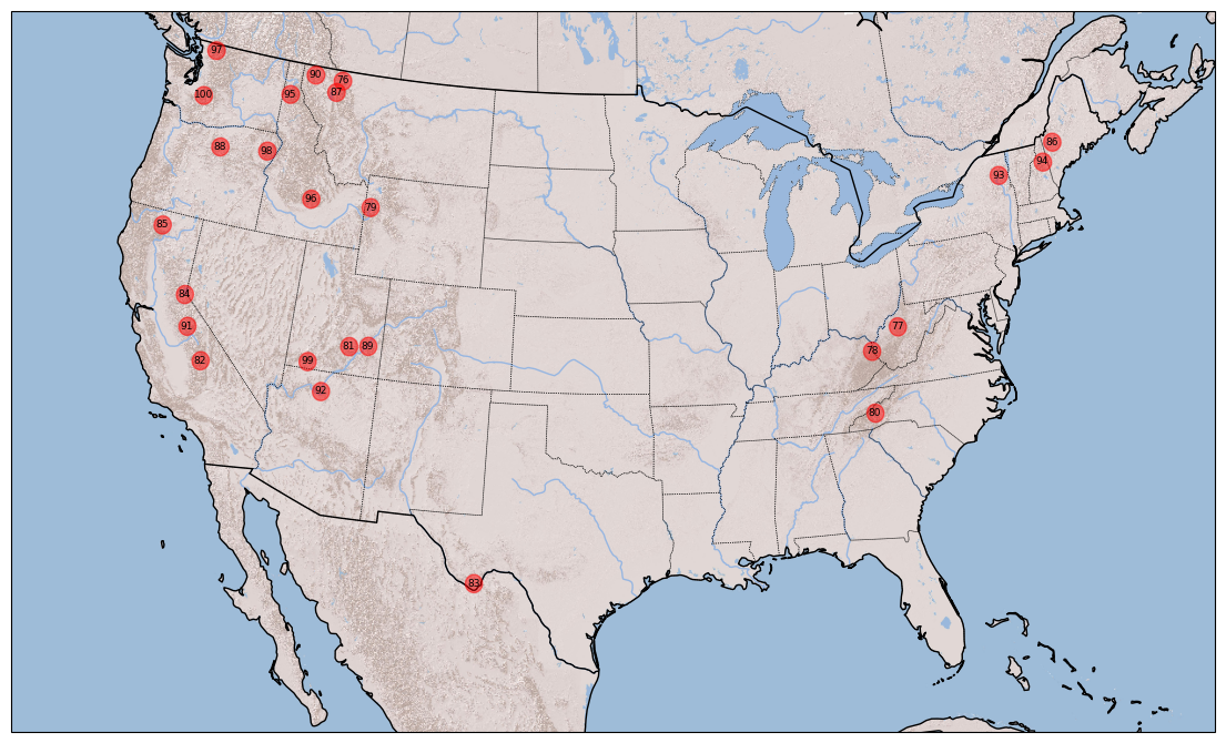
We categorize the scenarios in RASPNet into four subsets by difficulty: Basic scenarios, for , Intermediate scenarios, for , Challenging scenarios, for , and Eye-watering scenarios, where . These subsets are depicted in Figure 3 — the basic scenarios are largely concentrated in the Eastern United States and plains regions, having simpler clutter characteristics (e.g., the Bonneville Salt Flats). The intermediate scenarios have more uneven terrain than the basic scenarios, and encompass hillside regions, coastlines and valleys. The challenging scenarios are largely concentrated in the Western United States, comprising mountainous and variable terrain — this shift to more rugged and uneven terrain introduces clutter characteristics that deviate substantially from the baseline scenario. Lastly, the eye-watering scenarios are composed almost exclusively of mountainous terrain, canyons, and other diversified land types, representing scenarios with highly irregular and unpredictable clutter characteristics.
4 Dataset Applications
RASPNet has several applications relevant to the radar community. We describe two key applications in this section. Firstly, RASPNet can be used to benchmark data-driven algorithms for target localization against existing approaches. Secondly, RASPNet supports transfer learning in realistic radar scenarios, enabling the adaptation of pre-trained models to new environments — we demonstrate this via a toy example. Across both of these applications, we consider five example scenarios in RASPNet: Bonneville Salt Flats, UT () as the baseline scenario, Central Kansas, KS () from the Basic scenarios, the Ouachita Mountains, OK () from the Intermediate scenarios, the Great Smoky Mountains, TN () from the Challenging scenarios, and the Grand Canyon, AZ () from the Eye-watering scenarios, wherein . We first preprocess the RASPNet data via conventional RASP techniques, per Section 4.1. We compiled all results on a NVIDIA GeForce RTX 3090 GPU.
4.1 Data Preprocessing
To prepare RASPNet for the target localization and transfer learning tasks, we consider sub-regions from the scenarios, , which we call radar processing regions. The minimum and maximum range of each radar processing region from the airborne radar platform and the azimuth angle bounds of each radar processing region are provided in Table 3 (see Appendix Section C.1), and the range bin indices are , whereby . We run a set of independent experiments, where in each experiment, a point target is placed in range and azimuth, uniformly at random inside each radar processing region. We select the radar cross section (RCS) of each target independently at random from the uniform distribution, (dBsm), and we generate independent random realizations of the radar return for each target placement. We consider stationary targets in this example, with , wherein there is no Doppler processing. For compatibility with our generated target data, we divide the clutter realizations provided by RASPNet for scenario into separate clutter datasets with realizations, where . As , we only consider the first pulse from the clutter realizations. For the CVNN target localization benchmark task, we solely consider the first of the realizations, wherein . Using this construction, we now consider the signal model outlined in Section C.2 of the Appendix.
For both non-CVNN target localization and transfer learning tasks, we leverage datasets of heatmap matrices (Venkatasubramanian et al., 2023), which comprise test statistics obtained via the signal model from Appendix Section C.2, where . To produce each heatmap matrix, we sweep the radar steering vector, , across azimuth with step size , from to , producing an NAMF azimuth spectrum at each range bin. Arranging these spectra across the range bins gives a size matrix of NAMF test statistics. The values for and are in Table 3 for scenarios . The cumulative dataset contains heatmap matrices, formed using all combinations of and . For the CVNN target localization task, we consider -dimensional feature vectors, which are formed from the radar return data matrices described in Section C.2 of the Appendix, where . The cumulative dataset comprises the first feature vectors of the total combinations.
4.2 Target Localization Benchmark
Having obtained the datasets of heatmap matrices for scenarios , we benchmark the non-CVNN target localization performance of two existing algorithms — we consider the classical peak-cell midpoint algorithm outlined in (Venkatasubramanian et al., 2022), and compare it with the regression CNN architecture introduced in (Venkatasubramanian et al., 2023). We clarify that other classical algorithms exist for target localization, including gradient-based local search methods; these algorithms can also be benchmarked using RASPNet. The considered regression CNN architecture is further described in Section D.1 of the Appendix.
We now produce the training and test datasets for each scenario, . We partition each dataset of heatmap matrices such that the first examples form the training dataset, and the remaining examples form the test dataset. Let denote the range and azimuth of the midpoint of the peak heatmap matrix cell, and let denote the azimuth and velocity values predicted by the regression CNN, for example from our dataset for scenario . While our heatmap matrices follow the polar coordinate system, we can transform their ground truth target locations into Cartesian coordinates to report the localization error in meters, whereby and . Let be the ground truth target location and velocity for example from our dataset. For vector inputs , the localization error, , over the test examples, is defined as:
| (5) |
Regarding our case, , with for the peak cell midpoint , and for the regression CNN . For each scenario, , we train the regression CNN until convergence on the training dataset using MSE as our loss function, and we leverage the Adam optimizer (Kingma & Ba, 2014) with a learning rate of . The localization errors on the test dataset are summarized for the peak cell midpoint and the regression CNN in Table 1. We see that as the scenarios become more challenging — measured using the -statistic with respect to the baseline scenario — the localization performance of both methods worsen.
| (m) | (m) | -stat. | ||
|---|---|---|---|---|
| 1 | 29 | 21.62 0 | 9.88 0.50 | 0 |
| 4 | 60 | 21.83 0 | 14.60 0.82 | 3.51e-8 |
| 35 | 62 | 187.31 0 | 68.31 2.23 | 2.63e-7 |
| 57 | 76 | 360.53 0 | 145.34 5.91 | 7.91e-7 |
| 92 | 35 | 1004.20 0 | 220.45 9.67 | 4.04e-6 |
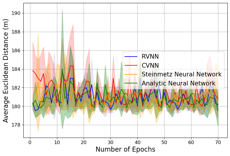
4.2.1 CVNN Target Localization Benchmark
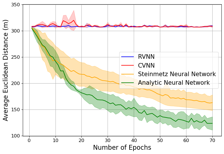
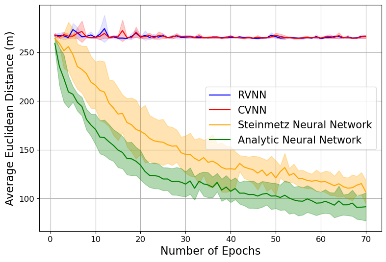
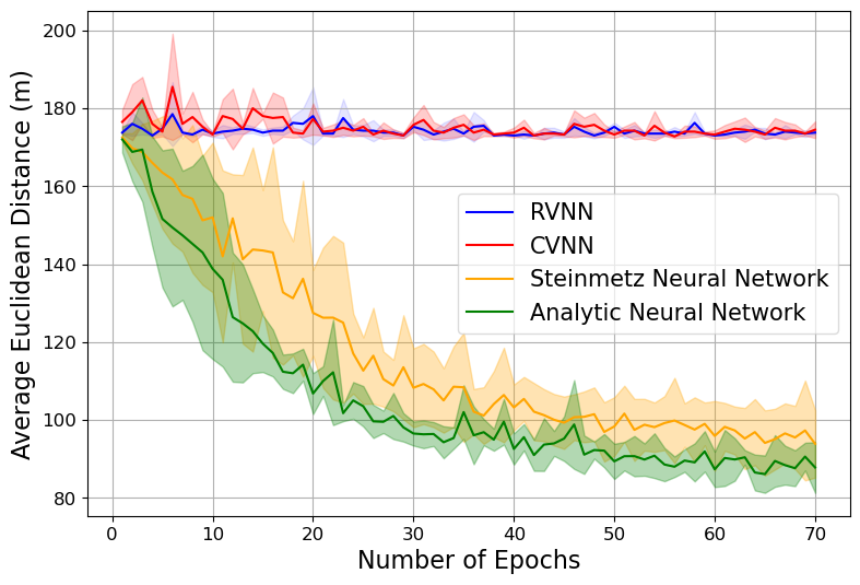
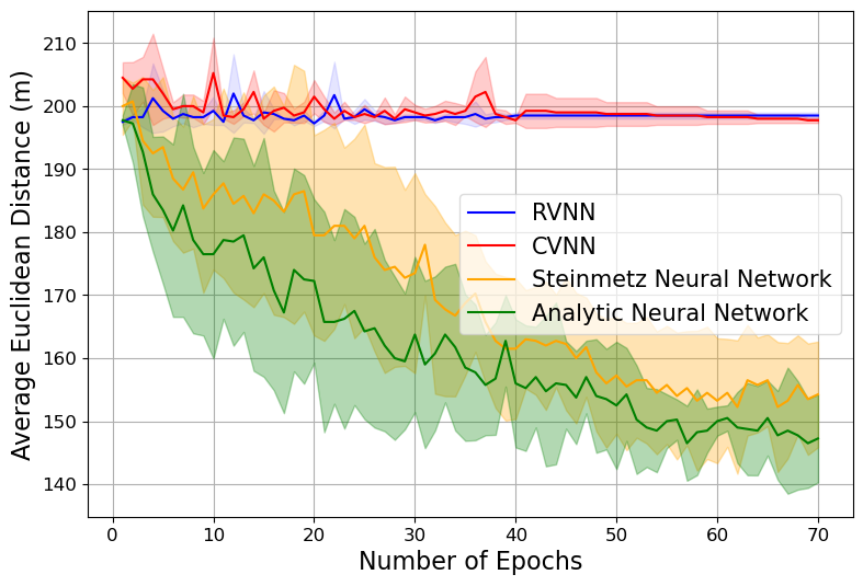
To benchmark the performance of CVNNs, we recall the datasets of feature vectors described in Section 4.1 for scenarios . Per (Trabelsi et al., 2017; Venkatasubramanian et al., 2024), we compare the performance of CVNNs and real-valued neural networks (RVNNs), versus Steinmetz and analytic neural networks (shown to achieve benchmark performance for complex-valued learning tasks). We partition each dataset of feature vectors such that the first examples form the training dataset, and the remaining examples form the test dataset. As our considered networks are regression CNN variants, we compute their localization errors via Eq. (5). For each scenario, , we train all networks until convergence on the training dataset using MSE as our loss function, and we leverage the Adam optimizer (Kingma & Ba, 2014) with a learning rate of . Per Figure 4, while the RVNN and CVNN are unable to learn the target localization task, the Steinmetz and analytic neural networks are able to effectively learn the task across all scenarios .
4.3 Transfer Learning
Apart from benchmarking the performance of algorithms, RASPNet can also be leveraged for transfer learning applications in realistic adaptive radar processing scenarios. We recall that the RFView®-generated data exhibits some degree of statistical similarity to real-world data, as examined in Section 2.4. As such, suppose we have collected clutter realizations, from some real-world scenario, , where . Suppose we also have neural networks trained for some predictive adaptive radar processing task on each of the RASPNet scenarios, . Our aim is to determine which of the trained neural networks should be chosen to achieve the best possible performance for the same task on the real-world scenario, . We can proceed by ranking the RASPNet scenarios, , by their similarity to scenario , using Algorithm 2. We hypothesize that the scenario with the lowest -statistic, relative to the real-world scenario, is the optimal choice for selecting the corresponding trained neural network. To improve the performance of this trained neural network on the real-world scenario, we can use a small number of samples from the real-world scenario to fine-tune it for the task at hand.
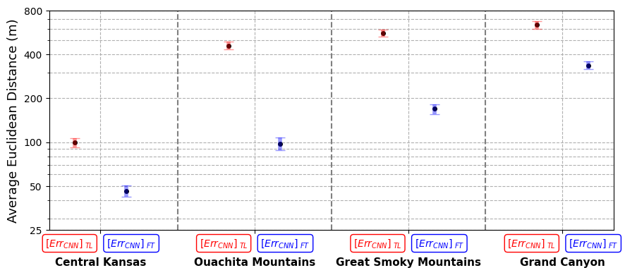
As a proof-of-concept, we again consider the non-CVNN target localization task, where we train our regression CNN to localize targets in scenario (Bonneville Salt Flats, UT). However, we evaluate this trained network on each of the scenarios to validate whether the scenario with the highest similarity to scenario from achieves the best localization performance. Paralleling Section 4.2, our training dataset comprises the first of the heatmap matrices generated for scenario . We consider four test datasets, each of which comprises the last of the total heatmap matrices generated for scenario , and we consider four datasets for fine-tuning, each of which comprises the first of the total heatmap matrices generated for scenario . We train the regression CNN on the training dataset using MSE as our loss function, and we leverage the Adam optimizer (Kingma & Ba, 2014) with . The localization accuracies on the test datasets, , , are depicted in Figure 5. As expected, the best performance is yielded by the neural network evaluated on the scenario (Central Kansas). This scenario has the lowest -statistic with respect to from .
We now consider the case of fine-tuning the trained regression CNN using a small set of heatmap matrices from the scenarios . We freeze the convolutional and batch normalization layers of our trained regression CNN, halving the number of parameters. Using the heatmap matrices, the weights and biases of the remaining layers are fine-tuned using MSE Loss and the Adam optimizer with . After fine-tuning the regression CNN for each scenario , we obtain the localization accuracies on the test datasets, , , depicted in Figure 5. We note that the improvements afforded by the regression CNN are largely recovered after fine-tuning.
5 Limitations and Other Applications
Apart from target localization, RASPNet serves as a comprehensive testbed for benchmarking adaptive radar target detection and classification algorithms. While it currently does not support target tracking capabilities, we plan to incorporate this feature in future work. A central limitation of RASPNet is the substantial size of its clutter datasets, with the entire dataset exceeding 16 TB and each scenario’s clutter data surpassing 160 GB. These large sizes are necessary to ensure sufficient resolution in range and Doppler and to provide ample clutter realizations for data-driven methods.
6 Conclusion
In this work, we presented RASPNet, a large-scale dataset for radar adaptive signal processing applications, consisting of scenarios across the contiguous United States with clutter realizations each. RASPNet provides a standardized benchmark for evaluating and developing RASP algorithms and complex-valued learning algorithms, bridging a significant gap in the availability of a comprehensive, realistic dataset for adaptive radar processing applications. We outlined relevant properties of RASPNet, described its organization, and provided two applications of the dataset for benchmarking target localization and transfer learning in realistic scenarios. Our experiments demonstrated RASPNet’s capability to support both traditional and data-driven approaches, highlighting its potential to accelerate research and development in the adaptive radar community.
Acknowledgements
This work was supported in part by the U.S. Air Force Office of Scientific Research (AFOSR) under award FA9550-21-1-0235. Dr. Muralidhar Rangaswamy and Dr. Bosung Kang were supported by AFOSR under project 20RYCORO51. The authors would like to thank the Sensors Directorate of the U.S. Air Force Research Laboratory for providing the radar sample of the Multi-Channel Airborne Radar Measurement (MCARM) program, and Dr. Erik Blasch at AFOSR for his continued support, which has made this effort possible. The opinions within this paper are the authors’ own and do not constitute any explicit or implicit endorsement by the U.S. Department of Defense.
References
- Babu et al. (1996) Babu, B. S., Torres, J. A., and Melvin, W. Processing and evaluation of multichannel airborne radar measurements (mcarm) measured data. In Proceedings of International Symposium on Phased Array Systems and Technology, pp. 395–399. IEEE, 1996.
- Blunt et al. (2006) Blunt, S. D., Gerlach, K., and Rangaswamy, M. Stap using knowledge-aided covariance estimation and the fracta algorithm. IEEE Transactions on Aerospace and Electronic Systems, 42(3):1043–1057, 2006.
- Brennan & Reed (1973) Brennan, L. and Reed, L. Theory of adaptive radar. IEEE Transactions on Aerospace and Electronic Systems, AES-9(2):237–252, 1973. doi: 10.1109/TAES.1973.309792.
- Crooks (2004) Crooks, S. Improving knowledge-aided stap performance using past cpi data [radar signal processing]. In Proceedings of the 2004 IEEE Radar Conference (IEEE Cat. No. 04CH37509), pp. 295–300. IEEE, 2004.
- Gogineni et al. (2022) Gogineni, S., Guerci, J. R., Nguyen, H. K., Bergin, J. S., Kirk, D. R., Watson, B. C., and Rangaswamy, M. High fidelity rf clutter modeling and simulation. IEEE Aerospace and Electronic Systems Magazine, 37(11):24–43, 2022. doi: 10.1109/MAES.2022.3208862.
- Guerci (2000) Guerci, J. R. Space-Time Adaptive Processing for Radar. Artech House, Norwood, MA, 2000.
- Guerci & Baranoski (2006) Guerci, J. R. and Baranoski, E. J. Knowledge-aided adaptive radar at darpa: an overview. IEEE Signal Processing Magazine, 23(1):41–50, 2006. doi: 10.1109/MSP.2006.1593336.
- Hara et al. (1994) Hara, Y., Atkins, R. G., Yueh, S. H., Shin, R. T., and Kong, J. A. Application of neural networks to radar image classification. IEEE Transactions on Geoscience and Remote Sensing, 32(1):100–109, 1994.
- Himed (1999) Himed, B. Mcarm/stap data analysis. volume ii. Volume II, 1999.
- Hirose et al. (2006) Hirose, A. et al. Complex-valued neural networks, volume 32. Wiley Online Library, 2006.
- Jiang et al. (2022) Jiang, W., Ren, Y., Liu, Y., and Leng, J. Artificial neural networks and deep learning techniques applied to radar target detection: A review. Electronics, 11(1):156, 2022.
- Johnson & Abramovich (2010) Johnson, B. A. and Abramovich, Y. I. Doa estimator performance assessment in the pre-asymptotic domain using the likelihood principle. Signal Processing, 90(5):1392–1401, 2010. ISSN 0165-1684. doi: https://doi.org/10.1016/j.sigpro.2009.11.006. Special Section on Statistical Signal & Array Processing.
- Kaufman & Rousseeuw (1990) Kaufman, L. and Rousseeuw, P. J. Partitioning Around Medoids (Program PAM), chapter 2, pp. 68–125. John Wiley & Sons, Ltd, 1990. ISBN 9780470316801. doi: https://doi.org/10.1002/9780470316801.ch2.
- Kingma & Ba (2014) Kingma, D. P. and Ba, J. Adam: A method for stochastic optimization. arXiv preprint arXiv:1412.6980, 2014.
- Klemm (2002) Klemm, R. Principles of Space-Time Adaptive Processing, volume 12. IET Radar, Sonar, Navigation and Avionics Series, London, UK, 2002.
- Li & Stoica (2008) Li, J. and Stoica, P. Advances in space-time adaptive processing. IEEE Transactions on Signal Processing, 56(6):2478–2497, 2008. doi: 10.1109/TSP.2008.917857.
- Matthès et al. (2021) Matthès, M. W., Bromberg, Y., de Rosny, J., and Popoff, S. M. Learning and avoiding disorder in multimode fibers. Phys. Rev. X, 11:021060, Jun 2021. doi: 10.1103/PhysRevX.11.021060. URL https://link.aps.org/doi/10.1103/PhysRevX.11.021060.
- Melvin (2004) Melvin, W. L. A stap overview. In IEEE Aerospace Conference, pp. 3–10, 2004. doi: 10.1109/AERO.2004.1367652.
- Mohammadi Asiyabi et al. (2023) Mohammadi Asiyabi, R., Datcu, M., Anghel, A., and Nies, H. Complex-valued end-to-end deep network with coherency preservation for complex-valued sar data reconstruction and classification. IEEE Transactions on Geoscience and Remote Sensing, 61:1–17, 2023. doi: 10.1109/TGRS.2023.3267185.
- Scardapane et al. (2020) Scardapane, S., Van Vaerenbergh, S., Hussain, A., and Uncini, A. Complex-valued neural networks with nonparametric activation functions. IEEE Transactions on Emerging Topics in Computational Intelligence, 4(2):140–150, 2020. doi: 10.1109/TETCI.2018.2872600.
- Stoica et al. (2008) Stoica, P., Li, J., Zhu, X., and Guerci, J. R. On using a priori knowledge in space-time adaptive processing. IEEE transactions on signal processing, 56(6):2598–2602, 2008.
- Székely & Rizzo (2013) Székely, G. J. and Rizzo, M. L. Energy statistics: A class of statistics based on distances. Journal of Statistical Planning and Inference, 143(8):1249–1272, 2013. ISSN 0378-3758. doi: https://doi.org/10.1016/j.jspi.2013.03.018.
- Trabelsi et al. (2017) Trabelsi, C., Bilaniuk, O., Zhang, Y., Serdyuk, D., Subramanian, S., Santos, J. F., Mehri, S., Rostamzadeh, N., Bengio, Y., and Pal, C. J. Deep complex networks. arXiv preprint arXiv:1705.09792, 2017.
- Venkatasubramanian et al. (2022) Venkatasubramanian, S., Wongkamthong, C., Soltani, M., Kang, B., Gogineni, S., Pezeshki, A., Rangaswamy, M., and Tarokh, V. Toward data-driven stap radar. In 2022 IEEE Radar Conference (RadarConf22), pp. 1–5, 2022. doi: 10.1109/RadarConf2248738.2022.9764354.
- Venkatasubramanian et al. (2023) Venkatasubramanian, S., Gogineni, S., Kang, B., Pezeshki, A., Rangaswamy, M., and Tarokh, V. Data-driven target localization using adaptive radar processing and convolutional neural networks, 2023.
- Venkatasubramanian et al. (2024) Venkatasubramanian, S., Pezeshki, A., and Tarokh, V. Steinmetz neural networks for complex-valued data, 2024.
- Wang et al. (2009) Wang, P., Li, H., and Himed, B. A new parametric glrt for multichannel adaptive signal detection. IEEE Transactions on Signal Processing, 58(1):317–325, 2009.
- Ward (1995) Ward, J. Space-time adaptive processing for airborne radar. In 1995 International Conference on Acoustics, Speech, and Signal Processing, volume 5, pp. 2809–2812 vol.5, 1995. doi: 10.1109/ICASSP.1995.479429.
- Ward (1998) Ward, J. Space-time adaptive processing for airborne radar. 1998.
- Wicks et al. (2006) Wicks, M. C., Rangaswamy, M., Adve, R., and Hale, T. B. Space-time adaptive processing: A knowledge-based perspective for airborne radar. IEEE Signal Processing Magazine, 23(1):51–65, 2006.
- Wu et al. (2023) Wu, J.-H., Zhang, S.-Q., Jiang, Y., and Zhou, Z.-H. Complex-valued neurons can learn more but slower than real-valued neurons via gradient descent. pp. 23714–23747, 2023.
Appendix
Appendix A Exemplar Scenario Validation
Below, Figure 6 pertains to the validation of the exemplary nature of RASPNet scenarios. We observe that the geographic coverage of the representative scenarios yielded by PAM mirrors the geographic coverage of the scenarios in RASPNet, as a preliminary proof-of-concept.
Appendix B MCARM Radar Platform Parameters
The list of parameters pertaining to the airborne radar platform from the MCARM measured dataset are provided in this section (Babu et al., 1996). To simulate the clutter realizations for the RFView and bald-earth cases, we instantiate an airborne radar platform in RFView® utilizing the parameters provided in Table 2. The complete description of MCARM parameters is provided in (Himed, 1999).
| Parameter | Value |
|---|---|
| Carrier frequency | |
| Bandwidth | |
| Pulse Repetition Frequency | |
| Radar platform altitude | |
| Radar platform position (lat, lon) | |
| Radar platform aim location (lat, lon) | |
| Radar platform speed | |
| Range resolution | |
| Antenna element configuration {horizontal vertical} | |
| Number of receiver channels {horizontal vertical} | |
| Antenna element horizontal spacing | |
| Antenna element vertical spacing | |
| Number of pulses | |
| Transmitted waveform number of samples | |
| Total number of range bins | |
| Radar range swath |
Appendix C Data Preprocessing Addendum
C.1 Radar Processing Region Parameters
Provided below are the radar processing region parameters for the scenarios considered in Section 4 from the main text, where .
| Bonneville Salt Flats, UT () – Parameters | Values |
|---|---|
| Radar platform position (lat, lon) | |
| Radar platform aim location (lat, lon) | |
| Sub-region extrema range bin midpoints | |
| Sub-region extrema azimuths | |
| Central Kansas, KS () – Parameters | Values |
| Radar platform position (lat, lon) | |
| Radar platform aim location (lat, lon) | |
| Sub-region extrema range bin midpoints | |
| Sub-region extrema azimuths | |
| Ouachita Mountains, OK () – Parameters | Values |
| Radar platform position (lat, lon) | |
| Radar platform aim location (lat, lon) | |
| Sub-region extrema range bin midpoints | |
| Sub-region extrema azimuths | |
| Great Smoky Mountains, TN () – Parameters | Values |
| Radar platform position (lat, lon) | |
| Radar platform aim location (lat, lon) | |
| Sub-region extrema range bin midpoints | |
| Sub-region extrema azimuths | |
| Grand Canyon, AZ () – Parameters | Values |
| Radar platform position (lat, lon) | |
| Radar platform aim location (lat, lon) | |
| Sub-region extrema range bin midpoints | |
| Sub-region extrema azimuths |
C.2 Signal Model
Suppose that are the random variables describing the target, clutter, and noise for scenario , and suppose that , , and denote the target, clutter, and noise data for the independent random realization of the radar return for scenario . Recording , , we obtain . We denote as the matched filtered radar return data matrix associated with range bin . The columns of are dimensional vectors that are built by stacking -dimensional array measurements, obtained from the radar pulse transmissions — for each pulse return, we have independent realizations. We consider a fixed clutter-to-noise ratio (CNR) of dB. The radar return data matrix is given by:
| (6) |
Where if range bin contains a target and otherwise, is the target response matrix, is the clutter response matrix, and is the noise response matrix. For the CVNN benchmark target localization task, we permute and reshape this radar return data matrix to obtain a -dimensional feature vector, .
Let denote the receiver array steering vector, where is the azimuth angle variable and is the elevation angle variable. Let be the Doppler processing linear phase vector across pulses; that is, , where is the Doppler shift frequency. Accordingly, the effective space-time steering vector, , in azimuth, elevation, and Doppler for radar processing is:
| (7) |
Where denotes Kronecker product. Suppose now that is the true clutter-plus-noise covariance matrix obtained from , where . The sample clutter-plus-noise covariance matrix is computed as: . The NAMF test statistic, , at coordinates in range bin , for scenario , is given by:
| (8) |
When the radar platform is at a long range from the ground scene, the elevation angle, , is close to zero. We consider this to be the case in our provided RASPNet empirical experiments.
Appendix D Neural Network Architectures
D.1 Regression CNN
The regression CNN architecture, shown in Figure 7, is designed for radar processing areas with an azimuth extent of and an azimuth step size of . The radar processing areas consist of range bins. Thus, each input data sample to the CNN is a size heatmap matrix.
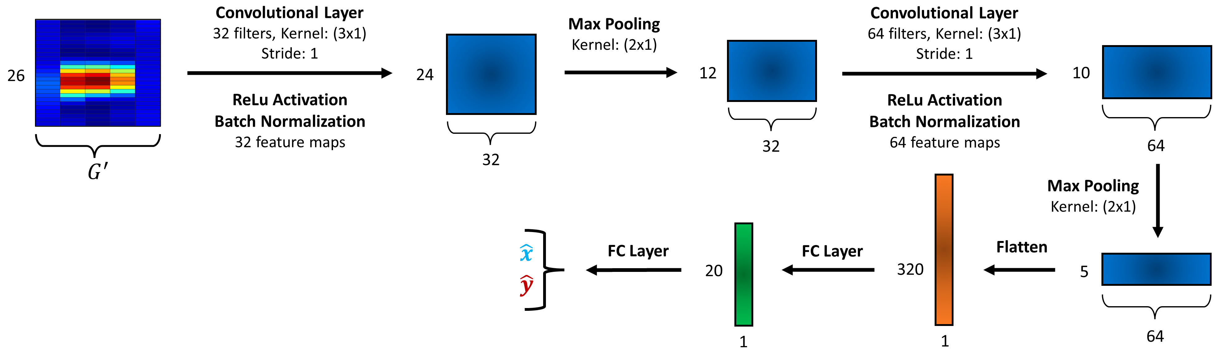
The input data first passes through a convolutional layer with a kernel and stride of 1, producing 32 feature maps, followed by ReLU activation and batch normalization. Max pooling is then applied with a kernel. This output goes through another convolutional layer with a kernel and stride of 1, producing 64 feature maps, again followed by ReLU activation, batch normalization, and max pooling utilizing a kernel. The output is flattened and passed through two fully connected layers to estimate the target location in range-azimuth coordinates, which is then converted to Cartesian coordinates .
D.2 Steinmetz Neural Network
The Steinmetz neural network is designed to handle both real and imaginary components of the input data separately before combining them for the final prediction. This architecture is evaluated on the CVNN benchmark from Section 4.2.1. The analytic neural network is a Steinmetz neural network in which the separately processed real and imaginary components are related by the discrete Hilbert transform (DHT), weighted by a tradeoff parameter, . Across all experiments in Section 4.2.1, we let , and consider , (see below).
-
•
Convolutional Layer (conv_real1): Applies a 2D convolution to the real input features, transforming them from -dimensional inputs to 32 feature maps using a kernel with padding 1, followed by a average pooling with stride 2 applied after activation.
-
•
ReLU Activation (real_relu1): Applies the ReLU activation function element-wise to the output of conv_real1.
-
•
Convolutional Layer (conv_real2): Applies a 2D convolution to the output of real_relu1, increasing feature maps from 32 to 64 using a kernel with padding 1, followed by a average pooling with stride 2 applied after activation.
-
•
ReLU Activation (real_relu2): Applies the ReLU activation function element-wise to the output of conv_real2.
-
•
Convolutional Layer (conv_imag1): Applies a 2D convolution to the imaginary input features, transforming them from -dimensional inputs to 32 feature maps using a kernel with padding 1, followed by a average pooling with stride 2 applied after activation.
-
•
ReLU Activation (imag_relu1): Applies the ReLU activation function element-wise to the output of conv_imag1.
-
•
Convolutional Layer (conv_imag2): Applies a 2D convolution to the output of imag_relu1, increasing feature maps from 32 to 64 using a kernel with padding 1, followed by a average pooling with stride 2 applied after activation.
-
•
ReLU Activation (imag_relu2): Applies the ReLU activation function element-wise to the output of conv_imag2.
-
•
Fully Connected Layer (fc1): Concatenates the flattened real and imaginary feature maps into a single vector and transforms it to an -dimensional latent space.
-
•
ReLU Activation (fcrelu1): Applies the ReLU activation function element-wise to the output of fc1.
-
•
Fully Connected Layer (fc2): Projects the -dimensional latent space to the final output dimension , producing the network’s prediction.
D.3 Real-Valued Neural Network
The real-valued neural network (RVNN) architecture is an approach for handling both real and imaginary components by concatenating them and processing them together. This architecture is evaluated on the CVNN benchmark from Section 4.2.1. Across all experiments in Section 4.2.1, we consider , (see below).
-
•
Convolutional Layer (conv1): Applies a 2D convolution to the concatenated real and imaginary input features, transforming them from -dimensional inputs to 32 feature maps using a kernel with padding 1, followed by a average pooling with stride 2 applied after activation.
-
•
ReLU Activation (relu1): Applies the ReLU activation function element-wise to the output of conv1.
-
•
Convolutional Layer (conv2): Applies a 2D convolution to the output of relu1, increasing feature maps from 32 to 64 using a kernel with padding 1, followed by a average pooling with stride 2 applied after activation.
-
•
ReLU Activation (relu2): Applies the ReLU activation function element-wise to the output of conv2.
-
•
Fully Connected Layer (fc1): Flattens the pooled feature maps into a single vector, transforming it to an -dimensional latent space.
-
•
ReLU Activation (fc_relu1): Applies the ReLU activation function element-wise to the output of fc1.
-
•
Fully Connected Layer (fc2): Projects the -dimensional latent space to the final output dimension , producing the network’s prediction.
D.4 Complex-Valued Neural Network
The Complex-Valued Neural Network (CVNN) is designed to handle complex-valued data by treating the real and imaginary parts jointly as complex numbers. To implement this network, we use the Complex PyTorch library (Matthès et al., 2021). This architecture is evaluated on the CVNN benchmark from Section 4.2.1. Across all experiments in Section 4.2.1, we consider , (see below).
-
•
Convolutional Layer (complex_conv1): Applies a 2D complex convolution to the complex-valued input features, transforming them from -dimensional inputs to 32 feature maps using a kernel with padding 1, followed by a average pooling with stride 2 applied after activation.
-
•
ReLU Activation (complex_relu1): Applies the complex ReLU activation function element-wise to the output of complex_conv1.
-
•
Convolutional Layer (complex_conv2): Applies a 2D complex convolution to the output of complex_relu1, increasing feature maps from 32 to 64 using a kernel with padding 1, followed by a complex average pooling with stride 2 applied after activation.
-
•
ReLU Activation (complex_relu2): Applies the complex ReLU activation function element-wise to the output of complex_conv2.
-
•
Fully Connected Layer (fc1): Flattens the pooled feature maps into a single vector, transforming it to an -dimensional latent space.
-
•
ReLU Activation (fc_relu1): Applies the complex ReLU activation function element-wise to the output of fc1.
-
•
Fully Connected Layer (fc2): Projects the -dimensional latent space to the final output dimension , producing the network’s prediction.
Appendix E Dataset and Code Access
E.1 Dataset Access and Organization
RASPNet is hosted within the Duke University Compute Cluster and can be accessed using the following Globus link: https://duke.is/8/jvkg. The dataset consists of radar scenarios from across the contiguous United States, each comprising clutter realizations. The main webpage for the dataset can be accessed at: https://shyamven.github.io/RASPNet.
The base folder in RASPNet contains three folders: EXAMPLES, CVNN, and CLUTTER. The EXAMPLES folder consists of data files used to generate the non-CVNN results presented in the main text, the CVNN folder consists of data files used to generate the CVNN results presented in the main text, and the CLUTTER folder consists of subfolders, each of which pertain to a different radar scenario. These scenarios are ordered from Westernmost to Easternmost, such that the folder CLUTTER/num1_lat_lon/ is the Westernmost scenario in RASPNet, and the folder CLUTTER/num100_lat_lon/ is the Easternmost scenario in RASPNet (lat and lon denote the platform latitude and longitude for each scenario). This nomenclature follows from the main text, where , and .
Each of the scenario subfolders in RASPNet contain i.i.d. clutter realizations, where each realization is stored within . The realization parallels from the main text, wherein , and . Importing the realization yields the variable X_clut, which is a size matrix.
The EXAMPLES folder consists of feature-labels pairs pertaining to five scenarios: . The features for scenario are stored in and the labels are stored in . These feature-label pairs were used to generate the non-CVNN target localization and transfer learning results from the main text, using the code files in Localization_Examples and Transfer_Learning_Examples (see Section E.2).
The CVNN folder consists of feature-labels pairs from five scenarios: . The train and test features for scenario are stored within in the folders and , and the labels are stored in and . These feature-label pairs were used to generate the CVNN target localization results from the main text using the code file RASPNet_CVNN.ipynb in Localization_Examples (see Section E.2).
E.2 Code Access
The code files for generating the empirical results provided within the main text can be found in the attached supplementary .zip file. We organize these files into two separate subfolders: Localization_Examples and Transfer_Learning_Examples. The Localization_Examples consist of code files for benchmarking non-CVNN and CVNN target localization accuracy in the scenarios . The Transfer_Learning_Examples consist of example transfer learning code files, where we train a regression neural network on scenario , and evaluate the network for .
Appendix F Datasheet
F.1 Motivation
-
1.
For what purpose was the dataset created? RASPNet was created to fill a noteworthy gap in the availability of a large-scale, realistic dataset to standardize the evaluation of adaptive radar processing techniques and support the development of data-driven complex-valued learning algorithms.
-
2.
Who created the dataset and on behalf of which entity? The dataset was created by a team of radar scientists and machine learning researchers provided in the author list.
-
3.
Who funded the creation of the dataset? The main funding body is the Air Force Office of Scientific Research.
F.2 Distribution
-
1.
Will the dataset be distributed to third parties outside of the entity (e.g., company) on behalf of which the dataset was created? Yes, the dataset is open to the public.
-
2.
How will the dataset will be distributed (e.g., tarball on website, API, GitHub)? The dataset can be downloaded using the provided Globus link and is hosted on the Duke University Compute Cluster.
-
3.
Have any third parties imposed IP-based or other restrictions on the data associated with the instances? No.
-
4.
Do any export controls or other regulatory restrictions apply to the dataset or to individual instances? No.
F.3 Maintenance
-
1.
Who will be supporting/hosting/maintaining the dataset? The authors, with the Duke University Office of Information Technology, will support, host, and maintain the dataset.
-
2.
Is there an erratum? No. If errors are found in the future, we will release errata on the main webpage for the dataset.
-
3.
Will the dataset be updated (e.g., to correct labeling errors, add new instances, delete instances)? Yes, the datasets will be updated whenever necessary to ensure accuracy, and announcements will be made accordingly. These updates will be posted on the main webpage for the dataset.
-
4.
Do the authors bear all responsibility in case of violation of rights, and confirm the data license?) Yes, the authors bear all responsibility in case of violation of rights.
-
5.
Will older version of the dataset continue to be supported/hosted/maintained? Yes, older versions of the dataset will continue to be maintained and hosted.
-
6.
If others want to extend/augment/build on/contribute to the dataset, is there a mechanisms for them to do so? No.
F.4 Composition
-
1.
What do the instance that comprise the dataset represent (e.g., documents, photos, people, countries?) RASPNet comprises airborne radar scenarios from across the contiguous United States. Each scenario consists of clutter realizations, which are stored as multidimensional matrices (.mat files).
-
2.
How many instances are there in total (of each type, if appropriate)? There are total clutter realizations present within RASPNet, amounting to more than TB of data.
-
3.
Does the dataset contain all possible instances or is it a sample of instances from a larger set? The dataset contains all possible instances of clutter realizations.
-
4.
Is there a label or target associated with each instance? The example code files provided alongside RASPNet have associated data files, which are stored in separate folders in RASPNet. These data files include feature-label pairs.
-
5.
Is any information missing from individual instances? No.
-
6.
Are there recommended data splits (e.g., training, development/validation, testing)? We do not have specific recommendations on the split within the training/validation set.
-
7.
Are there any errors, sources of noise, or redundancies in the dataset? RASPNet was generated using the RFView® modeling & simulation software, which incorporates thermal noise and other sources into the data generation process.
-
8.
Is the dataset self-contained, or does it link to or otherwise rely on external resources (e.g., websites, tweets, other datasets)? The dataset is self-contained.
-
9.
Does the dataset contain data that might be considered confidential? No.
-
10.
Does the dataset contain data that, if viewed directly, might be offensive, insulting, threatening, or might otherwise cause anxiety? No.
F.5 Collection Process
-
1.
How was the data associated with each instance acquired? The data associated with each realization was produced using the RFView® modeling and simulation software.
-
2.
What mechanisms or procedures were used to collect the data (e.g., hardware apparatus or sensor, manual human curation, software program, software API)? We used NVIDIA GeForce RTX 2080 and NVIDIA GeForce RTX 3090 GPU nodes in a high-performance computing cluster to run the RFView® simulations.
-
3.
Who was involved in the data collection process (e.g., students, crowdworkers, contractors) and how were they compensated (e.g., how much were crowdworkers paid)? Researchers at Duke University were involved in the data collection process. No crowdworkers were involved during the data collection process.
-
4.
Does the dataset relate to people? No.
-
5.
Did you collect the data from the individuals in questions directly, or obtain it via third parties or other sources (e.g., websites)? We obtained the dataset using the RFView® modeling and simulation software.
F.6 Uses
-
1.
Has the dataset been used for any tasks already? No, this dataset has not been used for any tasks yet, apart from the examples provided in the main text.
-
2.
Is there anything about the composition of the dataset or the way it was collected and preprocessed/cleaned/labeled that might impact future uses? The current composition of the dataset is self-sufficient, and any changes and updates made to the dataset will be documented via the dataset webpage.
-
3.
Are there tasks for which the dataset should not be used? No.
Appendix G Discussion of RASPNet Scenarios
We provide a complete tabulation of the scenarios comprising RASPNet, along with short descriptions, in this section. The scenarios are indexed by (difficulty), (Westernmost to Easternmost), and the airborne radar platform parameters are provided in Table 4.
G.1 Radar Platform Parameters
The full list of parameters pertaining to the airborne radar platform from the main text is provided below. This radar platform is used to obtain the clutter dataset for each scenario comprising RASPNet. We note that the radar processing region for each scenario is configured such that the aim location is halfway between the near range and far range, which is half of the radar range swath.
| Parameter | Value |
|---|---|
| Carrier frequency | |
| Bandwidth | |
| Pulse Repetition Frequency | |
| Radar platform altitude | |
| Range resolution | |
| Antenna element configuration {horizontal vertical} | |
| Number of receiver channels {horizontal vertical} | |
| Antenna element spacing | |
| Number of pulses | |
| Transmitted waveform number of samples | |
| Total number of range bins | |
| Radar range swath |
G.2 Basic Scenarios
We first outline the Basic RASPNet scenarios, where .
Scenario : Bonneville Salt Flats, UT ()
![[Uncaptioned image]](https://cdn.awesomepapers.org/papers/315d1b00-23f5-48a9-8f26-14e9ba83b4c3/num29.png) Platform Aim Location (lat, lon):
Platform Position (lat, lon):
Folder: /CLUTTER/num29_lat40.6391_lon-113.6525/
Description: Scenario in RASPNet is in the Bonneville Salt Flats region of Utah. The radar platform is positioned at latitude N and longitude W. It aims towards a location at latitude N and longitude W. This region is known for its minimal topographic relief, clear line of sight, and flat crust of salty soil.
Platform Aim Location (lat, lon):
Platform Position (lat, lon):
Folder: /CLUTTER/num29_lat40.6391_lon-113.6525/
Description: Scenario in RASPNet is in the Bonneville Salt Flats region of Utah. The radar platform is positioned at latitude N and longitude W. It aims towards a location at latitude N and longitude W. This region is known for its minimal topographic relief, clear line of sight, and flat crust of salty soil.
Scenario : Lake Michigan Coast, MI ()
![[Uncaptioned image]](https://cdn.awesomepapers.org/papers/315d1b00-23f5-48a9-8f26-14e9ba83b4c3/num72.png) Platform Aim Location (lat, lon):
Platform Position (lat, lon):
Folder: /CLUTTER/num72_lat42.295_lon-86.3169/
Description: Scenario in RASPNet is on the Lake Michigan coastline in Michigan. The radar platform is positioned at latitude N and longitude W. It aims towards a location at latitude N and longitude W. This is a land-to-water transition region with a flat coastline, where the aim location is on the water surface.
Platform Aim Location (lat, lon):
Platform Position (lat, lon):
Folder: /CLUTTER/num72_lat42.295_lon-86.3169/
Description: Scenario in RASPNet is on the Lake Michigan coastline in Michigan. The radar platform is positioned at latitude N and longitude W. It aims towards a location at latitude N and longitude W. This is a land-to-water transition region with a flat coastline, where the aim location is on the water surface.
Scenario : Charleston Harbor, SC ()
![[Uncaptioned image]](https://cdn.awesomepapers.org/papers/315d1b00-23f5-48a9-8f26-14e9ba83b4c3/num85.png) Platform Aim Location (lat, lon):
Platform Position (lat, lon):
Folder: /CLUTTER/num85_lat32.7996_lon-79.9423/
Description: Scenario in RASPNet is in the Charleston Harbor in South Carolina. The radar platform is positioned at latitude N and longitude W. It aims towards a location at latitude N and longitude W. This is a land-to-water transition region with a flat coastline, surrounding the Cooper River estuary.
Platform Aim Location (lat, lon):
Platform Position (lat, lon):
Folder: /CLUTTER/num85_lat32.7996_lon-79.9423/
Description: Scenario in RASPNet is in the Charleston Harbor in South Carolina. The radar platform is positioned at latitude N and longitude W. It aims towards a location at latitude N and longitude W. This is a land-to-water transition region with a flat coastline, surrounding the Cooper River estuary.
Scenario : Central Kansas, KS ()
![[Uncaptioned image]](https://cdn.awesomepapers.org/papers/315d1b00-23f5-48a9-8f26-14e9ba83b4c3/num60.png) Platform Aim Location (lat, lon):
Platform Position (lat, lon):
Folder: /CLUTTER/num60_lat37.9689_lon-97.575/
Description: Scenario in RASPNet is in the Great Plains region of Central Kansas. The radar platform is positioned at latitude N and longitude W. It aims towards a location at latitude N and longitude W. This region is characterized by an expansive and flat grassland environment, with low terrain variability.
Platform Aim Location (lat, lon):
Platform Position (lat, lon):
Folder: /CLUTTER/num60_lat37.9689_lon-97.575/
Description: Scenario in RASPNet is in the Great Plains region of Central Kansas. The radar platform is positioned at latitude N and longitude W. It aims towards a location at latitude N and longitude W. This region is characterized by an expansive and flat grassland environment, with low terrain variability.
Scenario : Texas Panhandle, TX ()
![[Uncaptioned image]](https://cdn.awesomepapers.org/papers/315d1b00-23f5-48a9-8f26-14e9ba83b4c3/num56.png) Platform Aim Location (lat, lon):
Platform Position (lat, lon):
Folder: /CLUTTER/num56_lat35.3487_lon-101.8228/
Description: Scenario in RASPNet is in the Great Plains region of panhandle Texas. The radar platform is positioned at latitude N and longitude W. It aims towards a location at latitude N and longitude W. This region is characterized by an expansive and flat grassland environment, with low terrain variability.
Platform Aim Location (lat, lon):
Platform Position (lat, lon):
Folder: /CLUTTER/num56_lat35.3487_lon-101.8228/
Description: Scenario in RASPNet is in the Great Plains region of panhandle Texas. The radar platform is positioned at latitude N and longitude W. It aims towards a location at latitude N and longitude W. This region is characterized by an expansive and flat grassland environment, with low terrain variability.
Scenario : Central Arkansas, AR ()
![[Uncaptioned image]](https://cdn.awesomepapers.org/papers/315d1b00-23f5-48a9-8f26-14e9ba83b4c3/num64.png) Platform Aim Location (lat, lon):
Platform Position (lat, lon):
Folder: /CLUTTER/num64_lat34.7491_lon-92.1178/
Description: Scenario in RASPNet is in the Arkansas River Valley of Central Arkansas. The radar platform is positioned at latitude N and longitude W. It aims towards a location at latitude N and longitude W. This region is characterized by flat lowlands and fertile farmlands, with low terrain variability.
Platform Aim Location (lat, lon):
Platform Position (lat, lon):
Folder: /CLUTTER/num64_lat34.7491_lon-92.1178/
Description: Scenario in RASPNet is in the Arkansas River Valley of Central Arkansas. The radar platform is positioned at latitude N and longitude W. It aims towards a location at latitude N and longitude W. This region is characterized by flat lowlands and fertile farmlands, with low terrain variability.
Scenario : Okefenokee Swamp, GA ()
![[Uncaptioned image]](https://cdn.awesomepapers.org/papers/315d1b00-23f5-48a9-8f26-14e9ba83b4c3/num81.png) Platform Aim Location (lat, lon):
Platform Position (lat, lon):
Folder: /CLUTTER/num81_lat31.1162_lon-82.4694/
Description: Scenario in RASPNet is in the Okefenokee Swamp of Southern Georgia. The radar platform is positioned at latitude N and longitude W. It aims towards a location at latitude N and longitude W. This region is characterized by a shallow and flat wetland environment, with low terrain variability.
Platform Aim Location (lat, lon):
Platform Position (lat, lon):
Folder: /CLUTTER/num81_lat31.1162_lon-82.4694/
Description: Scenario in RASPNet is in the Okefenokee Swamp of Southern Georgia. The radar platform is positioned at latitude N and longitude W. It aims towards a location at latitude N and longitude W. This region is characterized by a shallow and flat wetland environment, with low terrain variability.
Scenario : Lake Erie Coast, OH ()
![[Uncaptioned image]](https://cdn.awesomepapers.org/papers/315d1b00-23f5-48a9-8f26-14e9ba83b4c3/num78.png) Platform Aim Location (lat, lon):
Platform Position (lat, lon):
Folder: /CLUTTER/num78_lat41.6194_lon-83.1683/
Description: Scenario in RASPNet is on the Lake Erie coastline in Northern Ohio. The radar platform is positioned at latitude N and longitude W. It aims towards a location at latitude N and longitude W. This is a land-to-water transition region with a flat coastline, where the aim location is on the land surface.
Platform Aim Location (lat, lon):
Platform Position (lat, lon):
Folder: /CLUTTER/num78_lat41.6194_lon-83.1683/
Description: Scenario in RASPNet is on the Lake Erie coastline in Northern Ohio. The radar platform is positioned at latitude N and longitude W. It aims towards a location at latitude N and longitude W. This is a land-to-water transition region with a flat coastline, where the aim location is on the land surface.
Scenario : Algodones Dunes, CA ()
![[Uncaptioned image]](https://cdn.awesomepapers.org/papers/315d1b00-23f5-48a9-8f26-14e9ba83b4c3/num26.png) Platform Aim Location (lat, lon):
Platform Position (lat, lon):
Folder: /CLUTTER/num26_lat33.1031_lon-114.9343/
Description: Scenario in RASPNet is in the Algodones Dunes region of California. The radar platform is positioned at latitude N and longitude W. It aims towards a location at latitude N and longitude W. This region is characterized by a uniform desert environment, where the aim location is at the dune foothills.
Platform Aim Location (lat, lon):
Platform Position (lat, lon):
Folder: /CLUTTER/num26_lat33.1031_lon-114.9343/
Description: Scenario in RASPNet is in the Algodones Dunes region of California. The radar platform is positioned at latitude N and longitude W. It aims towards a location at latitude N and longitude W. This region is characterized by a uniform desert environment, where the aim location is at the dune foothills.
Scenario : Southern Indiana, IN ()
![[Uncaptioned image]](https://cdn.awesomepapers.org/papers/315d1b00-23f5-48a9-8f26-14e9ba83b4c3/num71.png) Platform Aim Location (lat, lon):
Platform Position (lat, lon):
Folder: /CLUTTER/num71_lat38.6645_lon-86.895/
Description: Scenario in RASPNet is in the Wabash Valley of Southern Indiana. The radar platform is positioned at latitude N and longitude W. It aims towards a location at latitude N and longitude W. This region is characterized by a uniform river valley environment with low elevation variability.
Platform Aim Location (lat, lon):
Platform Position (lat, lon):
Folder: /CLUTTER/num71_lat38.6645_lon-86.895/
Description: Scenario in RASPNet is in the Wabash Valley of Southern Indiana. The radar platform is positioned at latitude N and longitude W. It aims towards a location at latitude N and longitude W. This region is characterized by a uniform river valley environment with low elevation variability.
Scenario : Connecticut Coast, CT ()
![[Uncaptioned image]](https://cdn.awesomepapers.org/papers/315d1b00-23f5-48a9-8f26-14e9ba83b4c3/num95.png) Platform Aim Location (lat, lon):
Platform Position (lat, lon):
Folder: /CLUTTER/num95_lat41.2875_lon-72.6079/
Description: Scenario in RASPNet is on the Atlantic coastline of Connecticut. The radar platform is positioned at latitude N and longitude W. It aims towards a location at latitude N and longitude W. This is a land-to-water transition region with a flat coastline, where the aim location is on the water surface.
Platform Aim Location (lat, lon):
Platform Position (lat, lon):
Folder: /CLUTTER/num95_lat41.2875_lon-72.6079/
Description: Scenario in RASPNet is on the Atlantic coastline of Connecticut. The radar platform is positioned at latitude N and longitude W. It aims towards a location at latitude N and longitude W. This is a land-to-water transition region with a flat coastline, where the aim location is on the water surface.
Scenario : Southeastern New Mexico, NM ()
![[Uncaptioned image]](https://cdn.awesomepapers.org/papers/315d1b00-23f5-48a9-8f26-14e9ba83b4c3/num51.png) Platform Aim Location (lat, lon):
Platform Position (lat, lon):
Folder: /CLUTTER/num51_lat32.9892_lon-103.8644/
Description: Scenario in RASPNet is in the plains of Southeastern New Mexico. The radar platform is positioned at latitude N and longitude W. It aims towards a location at latitude N and longitude W. The radar platform is located above an escarpment overlooking and aiming towards a flat steppe region.
Platform Aim Location (lat, lon):
Platform Position (lat, lon):
Folder: /CLUTTER/num51_lat32.9892_lon-103.8644/
Description: Scenario in RASPNet is in the plains of Southeastern New Mexico. The radar platform is positioned at latitude N and longitude W. It aims towards a location at latitude N and longitude W. The radar platform is located above an escarpment overlooking and aiming towards a flat steppe region.
Scenario : San Joaquin Valley, CA ()
![[Uncaptioned image]](https://cdn.awesomepapers.org/papers/315d1b00-23f5-48a9-8f26-14e9ba83b4c3/num11.png) Platform Aim Location (lat, lon):
Platform Position (lat, lon):
Folder: /CLUTTER/num11_lat36.6554_lon-119.9324/
Description: Scenario in RASPNet is in the San Joaquin Valley of Central California. The radar platform is positioned at latitude N and longitude W. It aims towards a location at latitude N and longitude W. This region consists of a flat river valley, with fertile farmlands and low terrain variability.
Platform Aim Location (lat, lon):
Platform Position (lat, lon):
Folder: /CLUTTER/num11_lat36.6554_lon-119.9324/
Description: Scenario in RASPNet is in the San Joaquin Valley of Central California. The radar platform is positioned at latitude N and longitude W. It aims towards a location at latitude N and longitude W. This region consists of a flat river valley, with fertile farmlands and low terrain variability.
Scenario : San Francisco Bay, CA ()
![[Uncaptioned image]](https://cdn.awesomepapers.org/papers/315d1b00-23f5-48a9-8f26-14e9ba83b4c3/num3.png) Platform Aim Location (lat, lon):
Platform Position (lat, lon):
Folder: /CLUTTER/num3_lat37.7856_lon-122.4431/
Description: Scenario in RASPNet is in the San Francisco Bay area of California. The radar platform is positioned at latitude N and longitude W. It aims towards a location at latitude N and longitude W. This is a land-to-water transition region, where the aim direction is over a flatter section of coastline.
Platform Aim Location (lat, lon):
Platform Position (lat, lon):
Folder: /CLUTTER/num3_lat37.7856_lon-122.4431/
Description: Scenario in RASPNet is in the San Francisco Bay area of California. The radar platform is positioned at latitude N and longitude W. It aims towards a location at latitude N and longitude W. This is a land-to-water transition region, where the aim direction is over a flatter section of coastline.
Scenario : Lower Mississippi River, MS ()
![[Uncaptioned image]](https://cdn.awesomepapers.org/papers/315d1b00-23f5-48a9-8f26-14e9ba83b4c3/num68.png) Platform Aim Location (lat, lon):
Platform Position (lat, lon):
Folder: /CLUTTER/num68_lat33.8204_lon-90.7317/
Description: Scenario in RASPNet is on the Lower Mississippi River in Mississippi. The radar platform is positioned at latitude N and longitude W. It aims towards a location at latitude N and longitude W. This region is characteried by a flat river valley, with fertile farmlands and low terrain variability.
Platform Aim Location (lat, lon):
Platform Position (lat, lon):
Folder: /CLUTTER/num68_lat33.8204_lon-90.7317/
Description: Scenario in RASPNet is on the Lower Mississippi River in Mississippi. The radar platform is positioned at latitude N and longitude W. It aims towards a location at latitude N and longitude W. This region is characteried by a flat river valley, with fertile farmlands and low terrain variability.
Scenario : Saginaw Bay, MI ()
![[Uncaptioned image]](https://cdn.awesomepapers.org/papers/315d1b00-23f5-48a9-8f26-14e9ba83b4c3/num77.png) Platform Aim Location (lat, lon):
Platform Position (lat, lon):
Folder: /CLUTTER/num77_lat43.6216_lon-83.8388/
Description: Scenario in RASPNet is on the Saginaw Bay coastline of Michigan. The radar platform is positioned at latitude N and longitude W. It aims towards a location at latitude N and longitude W. The radar is positioned near the coastline, the aim direction is inland, and the surrounding terrain is flat.
Platform Aim Location (lat, lon):
Platform Position (lat, lon):
Folder: /CLUTTER/num77_lat43.6216_lon-83.8388/
Description: Scenario in RASPNet is on the Saginaw Bay coastline of Michigan. The radar platform is positioned at latitude N and longitude W. It aims towards a location at latitude N and longitude W. The radar is positioned near the coastline, the aim direction is inland, and the surrounding terrain is flat.
Scenario : Big Sur, CA ()
![[Uncaptioned image]](https://cdn.awesomepapers.org/papers/315d1b00-23f5-48a9-8f26-14e9ba83b4c3/num8.png) Platform Aim Location (lat, lon):
Platform Position (lat, lon):
Folder: /CLUTTER/num8_lat35.985_lon-121.4863/
Description: Scenario in RASPNet is in the Big Sur region of Coastal California. The radar platform is positioned at latitude N and longitude W. It aims towards a location at latitude N and longitude W. This is a land-to-water transition region, where the aim location is on the water surface and has low variability.
Platform Aim Location (lat, lon):
Platform Position (lat, lon):
Folder: /CLUTTER/num8_lat35.985_lon-121.4863/
Description: Scenario in RASPNet is in the Big Sur region of Coastal California. The radar platform is positioned at latitude N and longitude W. It aims towards a location at latitude N and longitude W. This is a land-to-water transition region, where the aim location is on the water surface and has low variability.
Scenario : Cape Cod, MA ()
![[Uncaptioned image]](https://cdn.awesomepapers.org/papers/315d1b00-23f5-48a9-8f26-14e9ba83b4c3/num100.png) Platform Aim Location (lat, lon):
Platform Position (lat, lon):
Folder: /CLUTTER/num100_lat41.7699_lon-70.0207/
Description: Scenario in RASPNet is in the Cape Cod region of Coastal Massachusetts. The radar platform is positioned at latitude N and longitude W. It aims towards a location at latitude N and longitude W. This is a land-to-water transition region, where the aim direction is over flat land with low variability.
Platform Aim Location (lat, lon):
Platform Position (lat, lon):
Folder: /CLUTTER/num100_lat41.7699_lon-70.0207/
Description: Scenario in RASPNet is in the Cape Cod region of Coastal Massachusetts. The radar platform is positioned at latitude N and longitude W. It aims towards a location at latitude N and longitude W. This is a land-to-water transition region, where the aim direction is over flat land with low variability.
Scenario : Delaware Bay, NJ ()
![[Uncaptioned image]](https://cdn.awesomepapers.org/papers/315d1b00-23f5-48a9-8f26-14e9ba83b4c3/num91.png) Platform Aim Location (lat, lon):
Platform Position (lat, lon):
Folder: /CLUTTER/num91_lat39.2179_lon-74.98/
Description: Scenario in RASPNet is on Delaware Bay in Southern New Jersey. The radar platform is positioned at latitude N and longitude W. It aims towards a location at latitude N and longitude W. This is a land-to-water transition region with a flat coastline, where the aim location is on the water surface.
Platform Aim Location (lat, lon):
Platform Position (lat, lon):
Folder: /CLUTTER/num91_lat39.2179_lon-74.98/
Description: Scenario in RASPNet is on Delaware Bay in Southern New Jersey. The radar platform is positioned at latitude N and longitude W. It aims towards a location at latitude N and longitude W. This is a land-to-water transition region with a flat coastline, where the aim location is on the water surface.
Scenario : Salt River Valley, AZ ()
![[Uncaptioned image]](https://cdn.awesomepapers.org/papers/315d1b00-23f5-48a9-8f26-14e9ba83b4c3/num36.png) Platform Aim Location (lat, lon):
Platform Position (lat, lon):
Folder: /CLUTTER/num36_lat33.4143_lon-111.4949/
Description: Scenario in RASPNet is in the Salt River Valley in Central Arizona. The radar platform is positioned at latitude N and longitude W. It aims towards a location at latitude N and longitude W. This region is characterized by an expansive and flat desert environment, with low terrain variability.
Platform Aim Location (lat, lon):
Platform Position (lat, lon):
Folder: /CLUTTER/num36_lat33.4143_lon-111.4949/
Description: Scenario in RASPNet is in the Salt River Valley in Central Arizona. The radar platform is positioned at latitude N and longitude W. It aims towards a location at latitude N and longitude W. This region is characterized by an expansive and flat desert environment, with low terrain variability.
Scenario : Snake River Plain, ID ()
![[Uncaptioned image]](https://cdn.awesomepapers.org/papers/315d1b00-23f5-48a9-8f26-14e9ba83b4c3/num30.png) Platform Aim Location (lat, lon):
Platform Position (lat, lon):
Folder: /CLUTTER/num30_lat43.3357_lon-113.6419/
Description: Scenario in RASPNet is in the Snake River Plain in Central Idaho. The radar platform is positioned at latitude N and longitude W. It aims towards a location at latitude N and longitude W. This region is characterized by a uniform and flat grassland environment, with low terrain variability.
Platform Aim Location (lat, lon):
Platform Position (lat, lon):
Folder: /CLUTTER/num30_lat43.3357_lon-113.6419/
Description: Scenario in RASPNet is in the Snake River Plain in Central Idaho. The radar platform is positioned at latitude N and longitude W. It aims towards a location at latitude N and longitude W. This region is characterized by a uniform and flat grassland environment, with low terrain variability.
Scenario : Badlands National Park, SD ()
![[Uncaptioned image]](https://cdn.awesomepapers.org/papers/315d1b00-23f5-48a9-8f26-14e9ba83b4c3/num55.png) Platform Aim Location (lat, lon):
Platform Position (lat, lon):
Folder: /CLUTTER/num55_lat43.8194_lon-102.3491/
Description: Scenario in RASPNet is in Badlands National Park in South Dakota. The radar platform is located at latitude N and longitude W. It aims towards a location at latitude N and longitude W. While this region is characterized by rough terrain, the aim location has low elevation variability.
Platform Aim Location (lat, lon):
Platform Position (lat, lon):
Folder: /CLUTTER/num55_lat43.8194_lon-102.3491/
Description: Scenario in RASPNet is in Badlands National Park in South Dakota. The radar platform is located at latitude N and longitude W. It aims towards a location at latitude N and longitude W. While this region is characterized by rough terrain, the aim location has low elevation variability.
Scenario : Chesapeake Bay, VA ()
![[Uncaptioned image]](https://cdn.awesomepapers.org/papers/315d1b00-23f5-48a9-8f26-14e9ba83b4c3/num90.png) Platform Aim Location (lat, lon):
Platform Position (lat, lon):
Folder: /CLUTTER/num90_lat37.84_lon-76.2766/
Description: Scenario in RASPNet is in the Chesapeake Bay region of Coastal Virginia. The radar platform is positioned at latitude N and longitude W. It aims towards a location at latitude N and longitude W. This is a land-to-water transition region, where the aim direction is over flat land with low variability.
Platform Aim Location (lat, lon):
Platform Position (lat, lon):
Folder: /CLUTTER/num90_lat37.84_lon-76.2766/
Description: Scenario in RASPNet is in the Chesapeake Bay region of Coastal Virginia. The radar platform is positioned at latitude N and longitude W. It aims towards a location at latitude N and longitude W. This is a land-to-water transition region, where the aim direction is over flat land with low variability.
Scenario : Lake Champlain, VT ()
![[Uncaptioned image]](https://cdn.awesomepapers.org/papers/315d1b00-23f5-48a9-8f26-14e9ba83b4c3/num93.png) Platform Aim Location (lat, lon):
Platform Position (lat, lon):
Folder: /CLUTTER/num93_lat44.6815_lon-73.3225/
Description: Scenario in RASPNet is in the Lake Champlain region of Vermont. The radar platform is positioned at latitude N and longitude W. It aims towards a location at latitude N and longitude W. This is a land-to-water transition region, where the aim direction is over water and has low variability.
Platform Aim Location (lat, lon):
Platform Position (lat, lon):
Folder: /CLUTTER/num93_lat44.6815_lon-73.3225/
Description: Scenario in RASPNet is in the Lake Champlain region of Vermont. The radar platform is positioned at latitude N and longitude W. It aims towards a location at latitude N and longitude W. This is a land-to-water transition region, where the aim direction is over water and has low variability.
Scenario : Santa Barbara Coast, CA ()
![[Uncaptioned image]](https://cdn.awesomepapers.org/papers/315d1b00-23f5-48a9-8f26-14e9ba83b4c3/num12.png) Platform Aim Location (lat, lon):
Platform Position (lat, lon):
Folder: /CLUTTER/num12_lat34.4289_lon-119.767/
Description: Scenario in RASPNet is on the Santa Barbara Coast in California. The radar platform is positioned at latitude N and longitude W. It aims towards a location at latitude N and longitude W. This is a land-to-water transition region, where the aim location is on the water surface.
Platform Aim Location (lat, lon):
Platform Position (lat, lon):
Folder: /CLUTTER/num12_lat34.4289_lon-119.767/
Description: Scenario in RASPNet is on the Santa Barbara Coast in California. The radar platform is positioned at latitude N and longitude W. It aims towards a location at latitude N and longitude W. This is a land-to-water transition region, where the aim location is on the water surface.
G.3 Intermediate Scenarios
We now outline the Intermediate RASPNet scenarios, where .
Scenario : Red River Valley, ND ()
![[Uncaptioned image]](https://cdn.awesomepapers.org/papers/315d1b00-23f5-48a9-8f26-14e9ba83b4c3/num61.png) Platform Aim Location (lat, lon):
Platform Position (lat, lon):
Folder: /CLUTTER/num61_lat47.1179_lon-96.8311/
Description: Scenario in RASPNet is in the Red River Valley in Eastern North Dakota. The radar platform is positioned at latitude N and longitude W. It aims towards a location at latitude N and longitude W. This region is characterized by a uniform and flat grassland environment, with low terrain variability.
Platform Aim Location (lat, lon):
Platform Position (lat, lon):
Folder: /CLUTTER/num61_lat47.1179_lon-96.8311/
Description: Scenario in RASPNet is in the Red River Valley in Eastern North Dakota. The radar platform is positioned at latitude N and longitude W. It aims towards a location at latitude N and longitude W. This region is characterized by a uniform and flat grassland environment, with low terrain variability.
Scenario : Superior Upland, WI ()
![[Uncaptioned image]](https://cdn.awesomepapers.org/papers/315d1b00-23f5-48a9-8f26-14e9ba83b4c3/num67.png) Platform Aim Location (lat, lon):
Platform Position (lat, lon):
Folder: /CLUTTER/num67_lat45.5059_lon-90.8222/
Description: Scenario in RASPNet is in the Superior Upland region of Wisconsin. The radar platform is located at latitude N and longitude W. It aims towards a location at latitude N and longitude W. While this region is characterized by nonuniform terrain, the aim location has low elevation variability.
Platform Aim Location (lat, lon):
Platform Position (lat, lon):
Folder: /CLUTTER/num67_lat45.5059_lon-90.8222/
Description: Scenario in RASPNet is in the Superior Upland region of Wisconsin. The radar platform is located at latitude N and longitude W. It aims towards a location at latitude N and longitude W. While this region is characterized by nonuniform terrain, the aim location has low elevation variability.
Scenario : Lake Erie Coast, PA ()
![[Uncaptioned image]](https://cdn.awesomepapers.org/papers/315d1b00-23f5-48a9-8f26-14e9ba83b4c3/num84.png) Platform Aim Location (lat, lon):
Platform Position (lat, lon):
Folder: /CLUTTER/num84_lat42.0964_lon-80.1729/
Description: Scenario in RASPNet is on the Lake Erie coastline of Pennsylvania. The radar platform is positioned at latitude N and longitude W. It aims towards a location at latitude N and longitude W. The radar is positioned near the coastline, the aim direction is inland, with nonuniform terrain.
Platform Aim Location (lat, lon):
Platform Position (lat, lon):
Folder: /CLUTTER/num84_lat42.0964_lon-80.1729/
Description: Scenario in RASPNet is on the Lake Erie coastline of Pennsylvania. The radar platform is positioned at latitude N and longitude W. It aims towards a location at latitude N and longitude W. The radar is positioned near the coastline, the aim direction is inland, with nonuniform terrain.
Scenario : Allegheny Plateau, PA ()
![[Uncaptioned image]](https://cdn.awesomepapers.org/papers/315d1b00-23f5-48a9-8f26-14e9ba83b4c3/num86.png) Platform Aim Location (lat, lon):
Platform Position (lat, lon):
Folder: /CLUTTER/num86_lat40.7_lon-79.6343/
Description: Scenario in RASPNet is in the Allegheny Plateau of Pennsylvania. The radar platform is positioned at latitude N and longitude W. It aims towards a location at latitude N and longitude W. While this region is characterized by nonuniform terrain, the aim location has low elevation variability.
Platform Aim Location (lat, lon):
Platform Position (lat, lon):
Folder: /CLUTTER/num86_lat40.7_lon-79.6343/
Description: Scenario in RASPNet is in the Allegheny Plateau of Pennsylvania. The radar platform is positioned at latitude N and longitude W. It aims towards a location at latitude N and longitude W. While this region is characterized by nonuniform terrain, the aim location has low elevation variability.
Scenario : North Georgia Mountains, GA ()
![[Uncaptioned image]](https://cdn.awesomepapers.org/papers/315d1b00-23f5-48a9-8f26-14e9ba83b4c3/num73.png) Platform Aim Location (lat, lon):
Platform Position (lat, lon):
Folder: /CLUTTER/num73_lat34.4884_lon-85.4009/
Description: Scenario in RASPNet is in mountainous Northern Georgia. The radar platform is located at latitude N and longitude W. It aims towards a location at latitude N and longitude W. While this region consists of rough terrain, the radar position and aim location is in a flat valley between ridges.
Platform Aim Location (lat, lon):
Platform Position (lat, lon):
Folder: /CLUTTER/num73_lat34.4884_lon-85.4009/
Description: Scenario in RASPNet is in mountainous Northern Georgia. The radar platform is located at latitude N and longitude W. It aims towards a location at latitude N and longitude W. While this region consists of rough terrain, the radar position and aim location is in a flat valley between ridges.
Scenario : Southwestern Texas, TX ()
![[Uncaptioned image]](https://cdn.awesomepapers.org/papers/315d1b00-23f5-48a9-8f26-14e9ba83b4c3/num53.png) Platform Aim Location (lat, lon):
Platform Position (lat, lon):
Folder: /CLUTTER/num53_lat30.0978_lon-103.5585/
Description: Scenario in RASPNet is in the hills region of Southwestern Texas. The radar platform is positioned at latitude N and longitude W. It aims towards a location at latitude N and longitude W. This region consists of hilly terrain with more pronounced nonuniformities.
Platform Aim Location (lat, lon):
Platform Position (lat, lon):
Folder: /CLUTTER/num53_lat30.0978_lon-103.5585/
Description: Scenario in RASPNet is in the hills region of Southwestern Texas. The radar platform is positioned at latitude N and longitude W. It aims towards a location at latitude N and longitude W. This region consists of hilly terrain with more pronounced nonuniformities.
Scenario : Southern Texas, TX ()
![[Uncaptioned image]](https://cdn.awesomepapers.org/papers/315d1b00-23f5-48a9-8f26-14e9ba83b4c3/num59.png) Platform Aim Location (lat, lon):
Platform Position (lat, lon):
Folder: /CLUTTER/num59_lat26.8356_lon-98.4699/
Description: Scenario in RASPNet is in the brush and plains region of Southern Texas. The radar platform is positioned at latitude N and longitude W. It aims towards a location at latitude N and longitude W. This region is characterized by a uniform steppe environment, with minimal terrain variability.
Platform Aim Location (lat, lon):
Platform Position (lat, lon):
Folder: /CLUTTER/num59_lat26.8356_lon-98.4699/
Description: Scenario in RASPNet is in the brush and plains region of Southern Texas. The radar platform is positioned at latitude N and longitude W. It aims towards a location at latitude N and longitude W. This region is characterized by a uniform steppe environment, with minimal terrain variability.
Scenario : Oregon Coast, OR ()
![[Uncaptioned image]](https://cdn.awesomepapers.org/papers/315d1b00-23f5-48a9-8f26-14e9ba83b4c3/num2.png) Platform Aim Location (lat, lon):
Platform Position (lat, lon):
Folder: /CLUTTER/num2_lat44.1917_lon-124.0905/
Description: Scenario in RASPNet is in the Coast Mountains of the Oregon Coast. The radar platform is positioned at latitude N and longitude W. It aims towards a location at latitude N and longitude W. This is a land-to-water transition region, where the aim location is on the water surface.
Platform Aim Location (lat, lon):
Platform Position (lat, lon):
Folder: /CLUTTER/num2_lat44.1917_lon-124.0905/
Description: Scenario in RASPNet is in the Coast Mountains of the Oregon Coast. The radar platform is positioned at latitude N and longitude W. It aims towards a location at latitude N and longitude W. This is a land-to-water transition region, where the aim location is on the water surface.
Scenario : Great Basin, NV ()
![[Uncaptioned image]](https://cdn.awesomepapers.org/papers/315d1b00-23f5-48a9-8f26-14e9ba83b4c3/num13.png) Platform Aim Location (lat, lon):
Platform Position (lat, lon):
Folder: /CLUTTER/num13_lat41.9174_lon-119.7279/
Description: Scenario in RASPNet is in the Great Basin region of Northern Nevada. The radar platform is positioned at latitude N and longitude W. It aims towards a location at latitude N and longitude W. This region is known for its basin and range topography and has more pronounced nonuniformities.
Platform Aim Location (lat, lon):
Platform Position (lat, lon):
Folder: /CLUTTER/num13_lat41.9174_lon-119.7279/
Description: Scenario in RASPNet is in the Great Basin region of Northern Nevada. The radar platform is positioned at latitude N and longitude W. It aims towards a location at latitude N and longitude W. This region is known for its basin and range topography and has more pronounced nonuniformities.
Scenario : Ouachita Mountains, OK ()
![[Uncaptioned image]](https://cdn.awesomepapers.org/papers/315d1b00-23f5-48a9-8f26-14e9ba83b4c3/num62.png) Platform Aim Location (lat, lon):
Platform Position (lat, lon):
Folder: /CLUTTER/num62_lat34.556_lon-95.6221/
Description: Scenario in RASPNet is in the Ouachita Mountains of Oklahoma. The radar platform is positioned at latitude N and longitude W. It aims towards a location at latitude N and longitude W. This region is characterized by small mountains and hills, and has some terrain variability.
Platform Aim Location (lat, lon):
Platform Position (lat, lon):
Folder: /CLUTTER/num62_lat34.556_lon-95.6221/
Description: Scenario in RASPNet is in the Ouachita Mountains of Oklahoma. The radar platform is positioned at latitude N and longitude W. It aims towards a location at latitude N and longitude W. This region is characterized by small mountains and hills, and has some terrain variability.
Scenario : Narragansett Bay, RI ()
![[Uncaptioned image]](https://cdn.awesomepapers.org/papers/315d1b00-23f5-48a9-8f26-14e9ba83b4c3/num96.png) Platform Aim Location (lat, lon):
Platform Position (lat, lon):
Folder: /CLUTTER/num96_lat41.4469_lon-71.5895/
Description: Scenario in RASPNet is near Narragansett Bay in Rhode Island. The radar platform is positioned at latitude N and longitude W. It aims towards a location at latitude N and longitude W. This is a land-to-water transition region, where the aim location is on the coastline.
Platform Aim Location (lat, lon):
Platform Position (lat, lon):
Folder: /CLUTTER/num96_lat41.4469_lon-71.5895/
Description: Scenario in RASPNet is near Narragansett Bay in Rhode Island. The radar platform is positioned at latitude N and longitude W. It aims towards a location at latitude N and longitude W. This is a land-to-water transition region, where the aim location is on the coastline.
Scenario : Mobile Bay, AL ()
![[Uncaptioned image]](https://cdn.awesomepapers.org/papers/315d1b00-23f5-48a9-8f26-14e9ba83b4c3/num69.png) Platform Aim Location (lat, lon):
Platform Position (lat, lon):
Folder: /CLUTTER/num69_lat30.5163_lon-87.8938/
Description: Scenario in RASPNet is on the Mobile Bay coastline of Alabama. The radar platform is positioned at latitude N and longitude W. It aims towards a location at latitude N and longitude W. This is a land-to-water transition region, where the aim location is on the water surface.
Platform Aim Location (lat, lon):
Platform Position (lat, lon):
Folder: /CLUTTER/num69_lat30.5163_lon-87.8938/
Description: Scenario in RASPNet is on the Mobile Bay coastline of Alabama. The radar platform is positioned at latitude N and longitude W. It aims towards a location at latitude N and longitude W. This is a land-to-water transition region, where the aim location is on the water surface.
Scenario : Lake Ontario Coast, NY ()
![[Uncaptioned image]](https://cdn.awesomepapers.org/papers/315d1b00-23f5-48a9-8f26-14e9ba83b4c3/num89.png) Platform Aim Location (lat, lon):
Platform Position (lat, lon):
Folder: /CLUTTER/num89_lat43.4339_lon-76.4938/
Description: Scenario in RASPNet is on the Lake Ontario coastline of New York. The radar platform is positioned at latitude N and longitude W. It aims towards a location at latitude N and longitude W. The radar is positioned near the coastline, the aim direction is inland, and the terrain has some variability.
Platform Aim Location (lat, lon):
Platform Position (lat, lon):
Folder: /CLUTTER/num89_lat43.4339_lon-76.4938/
Description: Scenario in RASPNet is on the Lake Ontario coastline of New York. The radar platform is positioned at latitude N and longitude W. It aims towards a location at latitude N and longitude W. The radar is positioned near the coastline, the aim direction is inland, and the terrain has some variability.
Scenario : Central North Dakota, ND ()
![[Uncaptioned image]](https://cdn.awesomepapers.org/papers/315d1b00-23f5-48a9-8f26-14e9ba83b4c3/num57.png) Platform Aim Location (lat, lon):
Platform Position (lat, lon):
Folder: /CLUTTER/num57_lat47.1979_lon-99.8113/
Description: Scenario in RASPNet is in the central prairie region of North Dakota. The radar platform is positioned at latitude N and longitude W. It aims towards a location at latitude N and longitude W. This region is known for its grassland topography and lakes, wherein the terrain has some variability.
Platform Aim Location (lat, lon):
Platform Position (lat, lon):
Folder: /CLUTTER/num57_lat47.1979_lon-99.8113/
Description: Scenario in RASPNet is in the central prairie region of North Dakota. The radar platform is positioned at latitude N and longitude W. It aims towards a location at latitude N and longitude W. This region is known for its grassland topography and lakes, wherein the terrain has some variability.
Scenario : Salton Sea Coast, CA ()
![[Uncaptioned image]](https://cdn.awesomepapers.org/papers/315d1b00-23f5-48a9-8f26-14e9ba83b4c3/num24.png) Platform Aim Location (lat, lon):
Platform Position (lat, lon):
Folder: /CLUTTER/num24_lat33.4282_lon-115.5721/
Description: Scenario in RASPNet is on the Salton Sea coastline in California. The radar platform is positioned at latitude N and longitude W. It aims towards a location at latitude N and longitude W. The radar is located above a mountain ridge, and the aim location is on the water surface.
Platform Aim Location (lat, lon):
Platform Position (lat, lon):
Folder: /CLUTTER/num24_lat33.4282_lon-115.5721/
Description: Scenario in RASPNet is on the Salton Sea coastline in California. The radar platform is positioned at latitude N and longitude W. It aims towards a location at latitude N and longitude W. The radar is located above a mountain ridge, and the aim location is on the water surface.
Scenario : Colorado Plateau, NM ()
![[Uncaptioned image]](https://cdn.awesomepapers.org/papers/315d1b00-23f5-48a9-8f26-14e9ba83b4c3/num44.png) Platform Aim Location (lat, lon):
Platform Position (lat, lon):
Folder: /CLUTTER/num44_lat36.7282_lon-108.202/
Description: Scenario in RASPNet is in the Colorado Plateau in New Mexico. The radar platform is positioned at latitude N and longitude W. It aims towards a location at latitude N and longitude W. This region is known for its nonuniform topography, wherein the terrain has some variability.
Platform Aim Location (lat, lon):
Platform Position (lat, lon):
Folder: /CLUTTER/num44_lat36.7282_lon-108.202/
Description: Scenario in RASPNet is in the Colorado Plateau in New Mexico. The radar platform is positioned at latitude N and longitude W. It aims towards a location at latitude N and longitude W. This region is known for its nonuniform topography, wherein the terrain has some variability.
Scenario : Santa Monica Coast, CA ()
![[Uncaptioned image]](https://cdn.awesomepapers.org/papers/315d1b00-23f5-48a9-8f26-14e9ba83b4c3/num16.png) Platform Aim Location (lat, lon):
Platform Position (lat, lon):
Folder: /CLUTTER/num16_lat34.092_lon-118.6362/
Description: Scenario in RASPNet is on the Santa Monica coastline in California. The radar platform is positioned at latitude N and longitude W. It aims towards a location at latitude N and longitude W. The radar is located above a mountain ridge, and the aim location is on the water surface.
Platform Aim Location (lat, lon):
Platform Position (lat, lon):
Folder: /CLUTTER/num16_lat34.092_lon-118.6362/
Description: Scenario in RASPNet is on the Santa Monica coastline in California. The radar platform is positioned at latitude N and longitude W. It aims towards a location at latitude N and longitude W. The radar is located above a mountain ridge, and the aim location is on the water surface.
Scenario : Boston Mountains, AR ()
![[Uncaptioned image]](https://cdn.awesomepapers.org/papers/315d1b00-23f5-48a9-8f26-14e9ba83b4c3/num63.png) Platform Aim Location (lat, lon):
Platform Position (lat, lon):
Folder: /CLUTTER/num63_lat36.1641_lon-93.6476/
Description: Scenario in RASPNet is in the Boston Mountains region of Arkansas. The radar platform is positioned at latitude N and longitude W. It aims towards a location at latitude N and longitude W. This region is characterized by small mountains and hills, and has some terrain variability.
Platform Aim Location (lat, lon):
Platform Position (lat, lon):
Folder: /CLUTTER/num63_lat36.1641_lon-93.6476/
Description: Scenario in RASPNet is in the Boston Mountains region of Arkansas. The radar platform is positioned at latitude N and longitude W. It aims towards a location at latitude N and longitude W. This region is characterized by small mountains and hills, and has some terrain variability.
Scenario : Lake Superior Coast, WI ()
![[Uncaptioned image]](https://cdn.awesomepapers.org/papers/315d1b00-23f5-48a9-8f26-14e9ba83b4c3/num66.png) Platform Aim Location (lat, lon):
Platform Position (lat, lon):
Folder: /CLUTTER/num66_lat46.6932_lon-90.8629/
Description: Scenario in RASPNet is on the Lake Superior coastline in Wisconsin. The radar platform is positioned at latitude N and longitude W. It aims towards a location at latitude N and longitude W. The radar is positioned near the coastline, the aim direction is inland, and the terrain has some variability.
Platform Aim Location (lat, lon):
Platform Position (lat, lon):
Folder: /CLUTTER/num66_lat46.6932_lon-90.8629/
Description: Scenario in RASPNet is on the Lake Superior coastline in Wisconsin. The radar platform is positioned at latitude N and longitude W. It aims towards a location at latitude N and longitude W. The radar is positioned near the coastline, the aim direction is inland, and the terrain has some variability.
Scenario : Massachusetts Bay, MA ()
![[Uncaptioned image]](https://cdn.awesomepapers.org/papers/315d1b00-23f5-48a9-8f26-14e9ba83b4c3/num98.png) Platform Aim Location (lat, lon):
Platform Position (lat, lon):
Folder: /CLUTTER/num98_lat42.3328_lon-71.0494/
Description: Scenario in RASPNet is on the Massachusetts Bay coastline near Boston. The radar platform is positioned at latitude N and longitude W. It aims towards a location at latitude N and longitude W. The radar is positioned near the coastline, the aim direction is inland, and the terrain has some variability.
Platform Aim Location (lat, lon):
Platform Position (lat, lon):
Folder: /CLUTTER/num98_lat42.3328_lon-71.0494/
Description: Scenario in RASPNet is on the Massachusetts Bay coastline near Boston. The radar platform is positioned at latitude N and longitude W. It aims towards a location at latitude N and longitude W. The radar is positioned near the coastline, the aim direction is inland, and the terrain has some variability.
Scenario : The Everglades, FL ()
![[Uncaptioned image]](https://cdn.awesomepapers.org/papers/315d1b00-23f5-48a9-8f26-14e9ba83b4c3/num83.png) Platform Aim Location (lat, lon):
Platform Position (lat, lon):
Folder: /CLUTTER/num83_lat25.4352_lon-80.3665/
Description: Scenario in RASPNet is in the Everglades region of South Florida. The radar platform is positioned at latitude N and longitude W. It aims towards a location at latitude N and longitude W. This region is characterized by a shallow and flat wetland environment, with low terrain variability.
Platform Aim Location (lat, lon):
Platform Position (lat, lon):
Folder: /CLUTTER/num83_lat25.4352_lon-80.3665/
Description: Scenario in RASPNet is in the Everglades region of South Florida. The radar platform is positioned at latitude N and longitude W. It aims towards a location at latitude N and longitude W. This region is characterized by a shallow and flat wetland environment, with low terrain variability.
Scenario : Upper Peninsula, MI ()
![[Uncaptioned image]](https://cdn.awesomepapers.org/papers/315d1b00-23f5-48a9-8f26-14e9ba83b4c3/num70.png) Platform Aim Location (lat, lon):
Platform Position (lat, lon):
Folder: /CLUTTER/num70_lat46.5559_lon-87.4021/
Description: Scenario in RASPNet is in the Upper Peninsula region of Michigan. The radar platform is positioned at latitude N and longitude W. It aims towards a location at latitude N and longitude W. The radar is positioned near the coastline, the aim direction is inland, and the terrain has some variability.
Platform Aim Location (lat, lon):
Platform Position (lat, lon):
Folder: /CLUTTER/num70_lat46.5559_lon-87.4021/
Description: Scenario in RASPNet is in the Upper Peninsula region of Michigan. The radar platform is positioned at latitude N and longitude W. It aims towards a location at latitude N and longitude W. The radar is positioned near the coastline, the aim direction is inland, and the terrain has some variability.
Scenario : Sandia Crest, NM (
![[Uncaptioned image]](https://cdn.awesomepapers.org/papers/315d1b00-23f5-48a9-8f26-14e9ba83b4c3/num48.png) Platform Aim Location (lat, lon):
Platform Position (lat, lon):
Folder: /CLUTTER/num48_lat38.8275_lon-104.9488/
Description: Scenario in RASPNet is in the Sandia Mountains of New Mexico. The radar platform is positioned at latitude N and longitude W. It aims towards a location at latitude N and longitude W. This region is noted for its variable terrain, and the radar is positioned behind a mountain crest.
Platform Aim Location (lat, lon):
Platform Position (lat, lon):
Folder: /CLUTTER/num48_lat38.8275_lon-104.9488/
Description: Scenario in RASPNet is in the Sandia Mountains of New Mexico. The radar platform is positioned at latitude N and longitude W. It aims towards a location at latitude N and longitude W. This region is noted for its variable terrain, and the radar is positioned behind a mountain crest.
Scenario : Central Nebraska, NE ()
![[Uncaptioned image]](https://cdn.awesomepapers.org/papers/315d1b00-23f5-48a9-8f26-14e9ba83b4c3/num58.png) Platform Aim Location (lat, lon):
Platform Position (lat, lon):
Folder: /CLUTTER/num58_lat41.5587_lon-99.2293/
Description: Scenario in RASPNet is in the Great Plains of Central Nebraska. The radar platform is positioned at latitude N and longitude W. It aims towards a location at latitude N and longitude W. This region is characterized by an expansive steppe environment, with low terrain variability.
Platform Aim Location (lat, lon):
Platform Position (lat, lon):
Folder: /CLUTTER/num58_lat41.5587_lon-99.2293/
Description: Scenario in RASPNet is in the Great Plains of Central Nebraska. The radar platform is positioned at latitude N and longitude W. It aims towards a location at latitude N and longitude W. This region is characterized by an expansive steppe environment, with low terrain variability.
Scenario : Catoctin Mountains, MD ()
![[Uncaptioned image]](https://cdn.awesomepapers.org/papers/315d1b00-23f5-48a9-8f26-14e9ba83b4c3/num88.png) Platform Aim Location (lat, lon):
Platform Position (lat, lon):
Folder: /CLUTTER/num88_lat39.626_lon-77.4582/
Description: Scenario in RASPNet is in the Catoctin Mountains of Maryland. The radar platform is positioned at latitude N and longitude W. It aims towards a location at latitude N and longitude W. This region is characterized by mountainous terrain, with increased nonuniformity.
Platform Aim Location (lat, lon):
Platform Position (lat, lon):
Folder: /CLUTTER/num88_lat39.626_lon-77.4582/
Description: Scenario in RASPNet is in the Catoctin Mountains of Maryland. The radar platform is positioned at latitude N and longitude W. It aims towards a location at latitude N and longitude W. This region is characterized by mountainous terrain, with increased nonuniformity.
G.4 Challenging Scenarios
We now outline the Challenging RASPNet scenarios, where .
Scenario : Straits of Mackinac, MI ()
![[Uncaptioned image]](https://cdn.awesomepapers.org/papers/315d1b00-23f5-48a9-8f26-14e9ba83b4c3/num74.png) Platform Aim Location (lat, lon):
Platform Position (lat, lon):
Folder: /CLUTTER/num74_lat45.7183_lon-87.7585/
Description: Scenario in RASPNet is near the Straits of Mackinac in Michigan. The radar platform is positioned at latitude N and longitude W. It aims towards a location at latitude N and longitude W. The radar is positioned near the coastline, the aim direction is inland, and the terrain has moderate variability.
Platform Aim Location (lat, lon):
Platform Position (lat, lon):
Folder: /CLUTTER/num74_lat45.7183_lon-87.7585/
Description: Scenario in RASPNet is near the Straits of Mackinac in Michigan. The radar platform is positioned at latitude N and longitude W. It aims towards a location at latitude N and longitude W. The radar is positioned near the coastline, the aim direction is inland, and the terrain has moderate variability.
Scenario : Washburn Range, WY ()
![[Uncaptioned image]](https://cdn.awesomepapers.org/papers/315d1b00-23f5-48a9-8f26-14e9ba83b4c3/num40.png) Platform Aim Location (lat, lon):
Platform Position (lat, lon):
Folder: /CLUTTER/num40_lat44.8686_lon-110.5484/
Description: Scenario in RASPNet is in the Washburn Range of Wyoming. The radar platform is positioned at latitude N and longitude W. It aims towards a location at latitude N and longitude W. The radar is positioned above a mountain summit, and the aim location has moderate terrain variability.
Platform Aim Location (lat, lon):
Platform Position (lat, lon):
Folder: /CLUTTER/num40_lat44.8686_lon-110.5484/
Description: Scenario in RASPNet is in the Washburn Range of Wyoming. The radar platform is positioned at latitude N and longitude W. It aims towards a location at latitude N and longitude W. The radar is positioned above a mountain summit, and the aim location has moderate terrain variability.
Scenario : Colorado Plateau, CO ()
![[Uncaptioned image]](https://cdn.awesomepapers.org/papers/315d1b00-23f5-48a9-8f26-14e9ba83b4c3/num45.png) Platform Aim Location (lat, lon):
Platform Position (lat, lon):
Folder: /CLUTTER/num45_lat39.5681_lon-107.5332/
Description: Scenario in RASPNet is in the Colorado Plateau of Western Colorado. The radar platform is positioned at latitude N and longitude W. It aims towards a location at latitude N and longitude W. The radar is positioned above a ridge system, and the aim location has moderate terrain variability.
Platform Aim Location (lat, lon):
Platform Position (lat, lon):
Folder: /CLUTTER/num45_lat39.5681_lon-107.5332/
Description: Scenario in RASPNet is in the Colorado Plateau of Western Colorado. The radar platform is positioned at latitude N and longitude W. It aims towards a location at latitude N and longitude W. The radar is positioned above a ridge system, and the aim location has moderate terrain variability.
Scenario : Bryce Canyon National Park, UT ()
![[Uncaptioned image]](https://cdn.awesomepapers.org/papers/315d1b00-23f5-48a9-8f26-14e9ba83b4c3/num34.png) Platform Aim Location (lat, lon):
Platform Position (lat, lon):
Folder: /CLUTTER/num34_lat37.6477_lon-112.1292/
Description: Scenario in RASPNet is in Bryce Canyon National Park in Utah. The radar platform is positioned at latitude N and longitude W. It aims towards a location at latitude N and longitude W. The radar is positioned above a canyon system, and the aim location has moderate terrain variability.
Platform Aim Location (lat, lon):
Platform Position (lat, lon):
Folder: /CLUTTER/num34_lat37.6477_lon-112.1292/
Description: Scenario in RASPNet is in Bryce Canyon National Park in Utah. The radar platform is positioned at latitude N and longitude W. It aims towards a location at latitude N and longitude W. The radar is positioned above a canyon system, and the aim location has moderate terrain variability.
Scenario : Dry Falls, WA ()
![[Uncaptioned image]](https://cdn.awesomepapers.org/papers/315d1b00-23f5-48a9-8f26-14e9ba83b4c3/num15.png) Platform Aim Location (lat, lon):
Platform Position (lat, lon):
Folder: /CLUTTER/num15_lat47.5126_lon-119.4791/
Description: Scenario in RASPNet is in Dry Falls State Park in Central Washington. The radar platform is positioned at latitude N and longitude W. It aims towards a location at latitude N and longitude W. This scenario comprises the rugged Channeled Scablands region, and has moderate terrain variability.
Platform Aim Location (lat, lon):
Platform Position (lat, lon):
Folder: /CLUTTER/num15_lat47.5126_lon-119.4791/
Description: Scenario in RASPNet is in Dry Falls State Park in Central Washington. The radar platform is positioned at latitude N and longitude W. It aims towards a location at latitude N and longitude W. This scenario comprises the rugged Channeled Scablands region, and has moderate terrain variability.
Scenario : Great Salt Lake Coast, UT ()
![[Uncaptioned image]](https://cdn.awesomepapers.org/papers/315d1b00-23f5-48a9-8f26-14e9ba83b4c3/num33.png) Platform Aim Location (lat, lon):
Platform Position (lat, lon):
Folder: /CLUTTER/num33_lat40.6958_lon-112.2119/
Description: Scenario in RASPNet is near the Great Salt Lake coastline in Utah. The radar platform is positioned at latitude N and longitude W. It aims towards a location at latitude N and longitude W. The radar is positioned near the coastline above a mountain ridge, and the aim direction is inland.
Platform Aim Location (lat, lon):
Platform Position (lat, lon):
Folder: /CLUTTER/num33_lat40.6958_lon-112.2119/
Description: Scenario in RASPNet is near the Great Salt Lake coastline in Utah. The radar platform is positioned at latitude N and longitude W. It aims towards a location at latitude N and longitude W. The radar is positioned near the coastline above a mountain ridge, and the aim direction is inland.
Scenario : Great Smoky Mountains, TN ()
![[Uncaptioned image]](https://cdn.awesomepapers.org/papers/315d1b00-23f5-48a9-8f26-14e9ba83b4c3/num76.png) Platform Aim Location (lat, lon):
Platform Position (lat, lon):
Folder: /CLUTTER/num76_lat35.4121_lon-84.1288/
Description: Scenario in RASPNet is near Tennessee’s Great Smoky Mountains. The radar platform is positioned at latitude N and longitude W. It aims towards a location at latitude N and longitude W. The radar is located above a series of hills, and the aim location has moderate terrain variability.
Platform Aim Location (lat, lon):
Platform Position (lat, lon):
Folder: /CLUTTER/num76_lat35.4121_lon-84.1288/
Description: Scenario in RASPNet is near Tennessee’s Great Smoky Mountains. The radar platform is positioned at latitude N and longitude W. It aims towards a location at latitude N and longitude W. The radar is located above a series of hills, and the aim location has moderate terrain variability.
Scenario : Cumberland Mountains, TN ()
![[Uncaptioned image]](https://cdn.awesomepapers.org/papers/315d1b00-23f5-48a9-8f26-14e9ba83b4c3/num75.png) Platform Aim Location (lat, lon):
Platform Position (lat, lon):
Folder: /CLUTTER/num75_lat36.1301_lon-84.3984/
Description: Scenario in RASPNet is in the Cumberland Mountains of Tennessee. The radar platform is located at latitude N and longitude W. It aims towards a location at latitude N and longitude W. The radar is located above a mountain ridge, and the aim location has moderate terrain variability.
Platform Aim Location (lat, lon):
Platform Position (lat, lon):
Folder: /CLUTTER/num75_lat36.1301_lon-84.3984/
Description: Scenario in RASPNet is in the Cumberland Mountains of Tennessee. The radar platform is located at latitude N and longitude W. It aims towards a location at latitude N and longitude W. The radar is located above a mountain ridge, and the aim location has moderate terrain variability.
Scenario : Lake Pend Orielle Coast, ID ()
![[Uncaptioned image]](https://cdn.awesomepapers.org/papers/315d1b00-23f5-48a9-8f26-14e9ba83b4c3/num23.png) Platform Aim Location (lat, lon):
Platform Position (lat, lon):
Folder: /CLUTTER/num23_lat48.154_lon-116.2233/
Description: Scenario in RASPNet is near the Lake Pend Orielle coastline in Idaho. The radar platform is positioned at latitude N and longitude W. It aims towards a location at latitude N and longitude W. The radar is positioned near the coastline, and the aim direction is inland, located on a mountain ridge.
Platform Aim Location (lat, lon):
Platform Position (lat, lon):
Folder: /CLUTTER/num23_lat48.154_lon-116.2233/
Description: Scenario in RASPNet is near the Lake Pend Orielle coastline in Idaho. The radar platform is positioned at latitude N and longitude W. It aims towards a location at latitude N and longitude W. The radar is positioned near the coastline, and the aim direction is inland, located on a mountain ridge.
Scenario : Death Valley National Park ()
![[Uncaptioned image]](https://cdn.awesomepapers.org/papers/315d1b00-23f5-48a9-8f26-14e9ba83b4c3/num20.png) Platform Aim Location (lat, lon):
Platform Position (lat, lon):
Folder: /CLUTTER/num20_lat36.1558_lon-116.9164/
Description: Scenario in RASPNet is in California’s Death Valley National Park. The radar platform is located at latitude N and longitude W. It aims towards a location at latitude N and longitude W. The radar is positioned above the valley floor, and the aim location is the summit of a tall mountain ridge.
Platform Aim Location (lat, lon):
Platform Position (lat, lon):
Folder: /CLUTTER/num20_lat36.1558_lon-116.9164/
Description: Scenario in RASPNet is in California’s Death Valley National Park. The radar platform is located at latitude N and longitude W. It aims towards a location at latitude N and longitude W. The radar is positioned above the valley floor, and the aim location is the summit of a tall mountain ridge.
Scenario : Guadalupe Mountains, TX ()
![[Uncaptioned image]](https://cdn.awesomepapers.org/papers/315d1b00-23f5-48a9-8f26-14e9ba83b4c3/num49.png) Platform Aim Location (lat, lon):
Platform Position (lat, lon):
Folder: /CLUTTER/num49_lat31.8881_lon-104.8603/
Description: Scenario in RASPNet is in the Guadalupe Mountains of Western Texas. The radar platform is located at latitude N and longitude W. It aims towards a location at latitude N and longitude W. The radar is positioned above a mountain summit, with the aim location far below within a flat basin.
Platform Aim Location (lat, lon):
Platform Position (lat, lon):
Folder: /CLUTTER/num49_lat31.8881_lon-104.8603/
Description: Scenario in RASPNet is in the Guadalupe Mountains of Western Texas. The radar platform is located at latitude N and longitude W. It aims towards a location at latitude N and longitude W. The radar is positioned above a mountain summit, with the aim location far below within a flat basin.
Scenario : Misquah Hills, MN ()
![[Uncaptioned image]](https://cdn.awesomepapers.org/papers/315d1b00-23f5-48a9-8f26-14e9ba83b4c3/num65.png) Platform Aim Location (lat, lon):
Platform Position (lat, lon):
Folder: /CLUTTER/num65_lat47.2824_lon-91.2762/
Description: Scenario in RASPNet is near the Misquah Hills of Upper Minnesota. The radar platform is located at latitude N and longitude W. It aims towards a location at latitude N and longitude W. The radar is positioned above a rugged coastline, and the aim location is along the Lake Superior Coast.
Platform Aim Location (lat, lon):
Platform Position (lat, lon):
Folder: /CLUTTER/num65_lat47.2824_lon-91.2762/
Description: Scenario in RASPNet is near the Misquah Hills of Upper Minnesota. The radar platform is located at latitude N and longitude W. It aims towards a location at latitude N and longitude W. The radar is positioned above a rugged coastline, and the aim location is along the Lake Superior Coast.
Scenario : Big Snowy Mountains, MT ()
![[Uncaptioned image]](https://cdn.awesomepapers.org/papers/315d1b00-23f5-48a9-8f26-14e9ba83b4c3/num42.png) Platform Aim Location (lat, lon):
Platform Position (lat, lon):
Folder: /CLUTTER/num42_lat46.7789_lon-109.4308/
Description: Scenario in RASPNet is in the Big Snowy Mountains of Montana. The radar platform is positioned at latitude N and longitude W. It aims towards a location at latitude N and longitude W. The radar is positioned above a mountain summit, and the aim location has moderate terrain variability.
Platform Aim Location (lat, lon):
Platform Position (lat, lon):
Folder: /CLUTTER/num42_lat46.7789_lon-109.4308/
Description: Scenario in RASPNet is in the Big Snowy Mountains of Montana. The radar platform is positioned at latitude N and longitude W. It aims towards a location at latitude N and longitude W. The radar is positioned above a mountain summit, and the aim location has moderate terrain variability.
Scenario : Missouri River Country, MT ()
![[Uncaptioned image]](https://cdn.awesomepapers.org/papers/315d1b00-23f5-48a9-8f26-14e9ba83b4c3/num50.png) Platform Aim Location (lat, lon):
Platform Position (lat, lon):
Folder: /CLUTTER/num50_lat47.6532_lon-104.6441/
Description: Scenario in RASPNet is in the Missouri River Country of Montana. The radar platform is located at latitude N and longitude W. It aims towards a location at latitude N and longitude W. This region is characterized by a mixture of rugged terrain and nonuniform topography.
Platform Aim Location (lat, lon):
Platform Position (lat, lon):
Folder: /CLUTTER/num50_lat47.6532_lon-104.6441/
Description: Scenario in RASPNet is in the Missouri River Country of Montana. The radar platform is located at latitude N and longitude W. It aims towards a location at latitude N and longitude W. This region is characterized by a mixture of rugged terrain and nonuniform topography.
Scenario : Bear Lake, ID ()
![[Uncaptioned image]](https://cdn.awesomepapers.org/papers/315d1b00-23f5-48a9-8f26-14e9ba83b4c3/num37.png) Platform Aim Location (lat, lon):
Platform Position (lat, lon):
Folder: /CLUTTER/num37_lat42.1479_lon-111.3145/
Description: Scenario in RASPNet is near Bear Lake in Southeastern Idaho. The radar platform is located at latitude N and longitude W. It aims towards a location at latitude N and longitude W. The radar is positioned above the coastline, and the aim location is the summit of a tall mountain ridge.
Platform Aim Location (lat, lon):
Platform Position (lat, lon):
Folder: /CLUTTER/num37_lat42.1479_lon-111.3145/
Description: Scenario in RASPNet is near Bear Lake in Southeastern Idaho. The radar platform is located at latitude N and longitude W. It aims towards a location at latitude N and longitude W. The radar is positioned above the coastline, and the aim location is the summit of a tall mountain ridge.
Scenario : Sheep Mountain, WY ()
![[Uncaptioned image]](https://cdn.awesomepapers.org/papers/315d1b00-23f5-48a9-8f26-14e9ba83b4c3/num47.png) Platform Aim Location (lat, lon):
Platform Position (lat, lon):
Folder: /CLUTTER/num47_lat41.2041_lon-106.0017/
Description: Scenario in RASPNet is near Sheep Mountain in Southern Wyoming. The radar platform is positioned at latitude N and longitude W. It aims towards a location at latitude N and longitude W. The radar is positioned above a mountain summit, and the aim location has moderate terrain variability.
Platform Aim Location (lat, lon):
Platform Position (lat, lon):
Folder: /CLUTTER/num47_lat41.2041_lon-106.0017/
Description: Scenario in RASPNet is near Sheep Mountain in Southern Wyoming. The radar platform is positioned at latitude N and longitude W. It aims towards a location at latitude N and longitude W. The radar is positioned above a mountain summit, and the aim location has moderate terrain variability.
Scenario : Flume Canyon, UT ()
![[Uncaptioned image]](https://cdn.awesomepapers.org/papers/315d1b00-23f5-48a9-8f26-14e9ba83b4c3/num43.png) Platform Aim Location (lat, lon):
Platform Position (lat, lon):
Folder: /CLUTTER/num43_lat39.1789_lon-109.4223/
Description: Scenario in RASPNet is near Flume Canyon in Southeastern Utah. The radar platform is positioned at latitude N and longitude W. It aims towards a location at latitude N and longitude W. This region is characterized by rugged canyonlands, and the aim location has moderate terrain variability.
Platform Aim Location (lat, lon):
Platform Position (lat, lon):
Folder: /CLUTTER/num43_lat39.1789_lon-109.4223/
Description: Scenario in RASPNet is near Flume Canyon in Southeastern Utah. The radar platform is positioned at latitude N and longitude W. It aims towards a location at latitude N and longitude W. This region is characterized by rugged canyonlands, and the aim location has moderate terrain variability.
Scenario : Hells Canyon, OR ()
![[Uncaptioned image]](https://cdn.awesomepapers.org/papers/315d1b00-23f5-48a9-8f26-14e9ba83b4c3/num21.png) Platform Aim Location (lat, lon):
Platform Position (lat, lon):
Folder: /CLUTTER/num21_lat45.5724_lon-116.6787/
Description: Scenario in RASPNet is in Hells Canyon in Eastern Oregon. The radar platform is positioned at latitude N and longitude W. It aims towards a location at latitude N and longitude W. This region is characterized by rugged canyonlands, and the aim location has high terrain variability.
Platform Aim Location (lat, lon):
Platform Position (lat, lon):
Folder: /CLUTTER/num21_lat45.5724_lon-116.6787/
Description: Scenario in RASPNet is in Hells Canyon in Eastern Oregon. The radar platform is positioned at latitude N and longitude W. It aims towards a location at latitude N and longitude W. This region is characterized by rugged canyonlands, and the aim location has high terrain variability.
Scenario : Cape Flattery, WA ()
![[Uncaptioned image]](https://cdn.awesomepapers.org/papers/315d1b00-23f5-48a9-8f26-14e9ba83b4c3/num1.png) Platform Aim Location (lat, lon):
Platform Position (lat, lon):
Folder: /CLUTTER/num1_lat48.2995_lon-124.6272/
Description: Scenario in RASPNet is near Cape Flattery in Western Washington. The radar platform is positioned at latitude N and longitude W. It aims towards a location at latitude N and longitude W. This is a land-to-water transition region, where the aim location is near the Olympic Peninsula coastline.
Platform Aim Location (lat, lon):
Platform Position (lat, lon):
Folder: /CLUTTER/num1_lat48.2995_lon-124.6272/
Description: Scenario in RASPNet is near Cape Flattery in Western Washington. The radar platform is positioned at latitude N and longitude W. It aims towards a location at latitude N and longitude W. This is a land-to-water transition region, where the aim location is near the Olympic Peninsula coastline.
Scenario : Three Sisters, OR ()
![[Uncaptioned image]](https://cdn.awesomepapers.org/papers/315d1b00-23f5-48a9-8f26-14e9ba83b4c3/num6.png) Platform Aim Location (lat, lon):
Platform Position (lat, lon):
Folder: /CLUTTER/num6_lat44.0991_lon-121.7425/
Description: Scenario in RASPNet is near the Three Sisters peaks of Central Oregon. The radar platform is positioned at latitude N and longitude W. It aims towards a location at latitude N and longitude W. The radar is positioned above a mountain ridge, and the aim location has high terrain variability.
Platform Aim Location (lat, lon):
Platform Position (lat, lon):
Folder: /CLUTTER/num6_lat44.0991_lon-121.7425/
Description: Scenario in RASPNet is near the Three Sisters peaks of Central Oregon. The radar platform is positioned at latitude N and longitude W. It aims towards a location at latitude N and longitude W. The radar is positioned above a mountain ridge, and the aim location has high terrain variability.
Scenario : Black Hills, SD ()
![[Uncaptioned image]](https://cdn.awesomepapers.org/papers/315d1b00-23f5-48a9-8f26-14e9ba83b4c3/num52.png) Platform Aim Location (lat, lon):
Platform Position (lat, lon):
Folder: /CLUTTER/num52_lat44.0686_lon-103.7762/
Description: Scenario in RASPNet is in the Black Hills region of South Dakota. The radar platform is positioned at latitude N and longitude W. It aims towards a location at latitude N and longitude W. The radar is positioned above rugged mountains, and the aim location has high terrain variability.
Platform Aim Location (lat, lon):
Platform Position (lat, lon):
Folder: /CLUTTER/num52_lat44.0686_lon-103.7762/
Description: Scenario in RASPNet is in the Black Hills region of South Dakota. The radar platform is positioned at latitude N and longitude W. It aims towards a location at latitude N and longitude W. The radar is positioned above rugged mountains, and the aim location has high terrain variability.
Scenario : Palouse Hills, WA ()
![[Uncaptioned image]](https://cdn.awesomepapers.org/papers/315d1b00-23f5-48a9-8f26-14e9ba83b4c3/num18.png) Platform Aim Location (lat, lon):
Platform Position (lat, lon):
Folder: /CLUTTER/num18_lat46.8061_lon-117.549/
Description: Scenario in RASPNet is in the Palouse Hills of Eastern Washington. The radar platform is positioned at latitude N and longitude W. It aims towards a location at latitude N and longitude W. The radar is positioned above rolling hills, and the aim location has high terrain variability.
Platform Aim Location (lat, lon):
Platform Position (lat, lon):
Folder: /CLUTTER/num18_lat46.8061_lon-117.549/
Description: Scenario in RASPNet is in the Palouse Hills of Eastern Washington. The radar platform is positioned at latitude N and longitude W. It aims towards a location at latitude N and longitude W. The radar is positioned above rolling hills, and the aim location has high terrain variability.
Scenario : Appalachian Mountains, PA ()
![[Uncaptioned image]](https://cdn.awesomepapers.org/papers/315d1b00-23f5-48a9-8f26-14e9ba83b4c3/num87.png) Platform Aim Location (lat, lon):
Platform Position (lat, lon):
Folder: /CLUTTER/num87_lat39.96_lon-77.8444/
Description: Scenario in RASPNet is in the Appalachian Mountains in Pennsylvania. The radar platform is positioned at latitude N and longitude W. It aims towards a location at latitude N and longitude W. The radar is positioned above a mountain ridge, and the aim location has high terrain variability.
Platform Aim Location (lat, lon):
Platform Position (lat, lon):
Folder: /CLUTTER/num87_lat39.96_lon-77.8444/
Description: Scenario in RASPNet is in the Appalachian Mountains in Pennsylvania. The radar platform is positioned at latitude N and longitude W. It aims towards a location at latitude N and longitude W. The radar is positioned above a mountain ridge, and the aim location has high terrain variability.
Scenario : Pikes Peak, CO ()
Platform Aim Location (lat, lon):
Platform Position (lat, lon):
Folder: /CLUTTER/num48_lat38.8275_lon-104.9488/
Description: Scenario in RASPNet is near Pikes Peak in the Colorado Front Range. The radar platform is positioned at latitude N and longitude W. It aims towards a location at latitude N and longitude W. The radar is positioned behind a mountain ridge, and the aim location has high terrain variability.
Scenario : Mount Greylock, MA ()
![[Uncaptioned image]](https://cdn.awesomepapers.org/papers/315d1b00-23f5-48a9-8f26-14e9ba83b4c3/num94.png) Platform Aim Location (lat, lon):
Platform Position (lat, lon):
Folder: /CLUTTER/num94_lat42.6295_lon-73.1617/
Description: Scenario in RASPNet is near Mount Greylock in Western Massachusetts. The radar platform is positioned at latitude N and longitude W. It aims towards a location at latitude N and longitude W. The radar is positioned above a mountain summit, and the aim location has high terrain variability.
Platform Aim Location (lat, lon):
Platform Position (lat, lon):
Folder: /CLUTTER/num94_lat42.6295_lon-73.1617/
Description: Scenario in RASPNet is near Mount Greylock in Western Massachusetts. The radar platform is positioned at latitude N and longitude W. It aims towards a location at latitude N and longitude W. The radar is positioned above a mountain summit, and the aim location has high terrain variability.
G.5 Eye-watering Scenarios
Lastly, we outline the Eye-watering RASPNet scenarios, where .
Scenario : Glacier National Park, MT ()
![[Uncaptioned image]](https://cdn.awesomepapers.org/papers/315d1b00-23f5-48a9-8f26-14e9ba83b4c3/num31.png) Platform Aim Location (lat, lon):
Platform Position (lat, lon):
Folder: /CLUTTER/num31_lat48.5934_lon-113.5835/
Description: Scenario in RASPNet is in Glacier National Park in Western Montana. The radar platform is located at latitude N and longitude W. It aims towards a location at latitude N and longitude W. The radar is located above a mountain ridge, and the aim location is a canyon with high terrain variability.
Platform Aim Location (lat, lon):
Platform Position (lat, lon):
Folder: /CLUTTER/num31_lat48.5934_lon-113.5835/
Description: Scenario in RASPNet is in Glacier National Park in Western Montana. The radar platform is located at latitude N and longitude W. It aims towards a location at latitude N and longitude W. The radar is located above a mountain ridge, and the aim location is a canyon with high terrain variability.
Scenario : Allegheny Plateau, WV ()
![[Uncaptioned image]](https://cdn.awesomepapers.org/papers/315d1b00-23f5-48a9-8f26-14e9ba83b4c3/num82.png) Platform Aim Location (lat, lon):
Platform Position (lat, lon):
Folder: /CLUTTER/num82_lat38.9185_lon-81.0876/
Description: Scenario in RASPNet is in the Allegheny Plateau region of West Virginia. The radar platform is located at latitude N and longitude W. It aims towards a location at latitude N and longitude W. This region is characterized by a mixture of rugged terrain and nonuniform topography.
Platform Aim Location (lat, lon):
Platform Position (lat, lon):
Folder: /CLUTTER/num82_lat38.9185_lon-81.0876/
Description: Scenario in RASPNet is in the Allegheny Plateau region of West Virginia. The radar platform is located at latitude N and longitude W. It aims towards a location at latitude N and longitude W. This region is characterized by a mixture of rugged terrain and nonuniform topography.
Scenario : Cumberland Plateau, KY ()
![[Uncaptioned image]](https://cdn.awesomepapers.org/papers/315d1b00-23f5-48a9-8f26-14e9ba83b4c3/num80.png) Platform Aim Location (lat, lon):
Platform Position (lat, lon):
Folder: /CLUTTER/num80_lat38.0973_lon-82.647/
Description: Scenario in RASPNet is in the Cumberland Plateau region of Kentucky. The radar platform is located at latitude N and longitude W. It aims towards a location at latitude N and longitude W. This region is characterized by a mixture of rugged terrain and nonuniform topography.
Platform Aim Location (lat, lon):
Platform Position (lat, lon):
Folder: /CLUTTER/num80_lat38.0973_lon-82.647/
Description: Scenario in RASPNet is in the Cumberland Plateau region of Kentucky. The radar platform is located at latitude N and longitude W. It aims towards a location at latitude N and longitude W. This region is characterized by a mixture of rugged terrain and nonuniform topography.
Scenario : Grand Teton National Park, WY ()
![[Uncaptioned image]](https://cdn.awesomepapers.org/papers/315d1b00-23f5-48a9-8f26-14e9ba83b4c3/num39.png) Platform Aim Location (lat, lon):
Platform Position (lat, lon):
Folder: /CLUTTER/num39_lat43.733_lon-110.757/
Description: Scenario in RASPNet is in Grand Teton National Park in Wyoming. The radar platform is located at latitude N and longitude W. It aims towards a location at latitude N and longitude W. The radar is positioned at the base of a mountain, and the aim location has high terrain variability.
Platform Aim Location (lat, lon):
Platform Position (lat, lon):
Folder: /CLUTTER/num39_lat43.733_lon-110.757/
Description: Scenario in RASPNet is in Grand Teton National Park in Wyoming. The radar platform is located at latitude N and longitude W. It aims towards a location at latitude N and longitude W. The radar is positioned at the base of a mountain, and the aim location has high terrain variability.
Scenario : Blue Ridge Mountains, NC ()
![[Uncaptioned image]](https://cdn.awesomepapers.org/papers/315d1b00-23f5-48a9-8f26-14e9ba83b4c3/num79.png) Platform Aim Location (lat, lon):
Platform Position (lat, lon):
Folder: /CLUTTER/num79_lat35.6463_lon-82.8889/
Description: Scenario in RASPNet is in North Carolina’s Blue Ridge Mountains. The radar platform is located at latitude N and longitude W. It aims towards a location at latitude N and longitude W. The radar is positioned near a mountain ridge, and the aim location has high terrain variability.
Platform Aim Location (lat, lon):
Platform Position (lat, lon):
Folder: /CLUTTER/num79_lat35.6463_lon-82.8889/
Description: Scenario in RASPNet is in North Carolina’s Blue Ridge Mountains. The radar platform is located at latitude N and longitude W. It aims towards a location at latitude N and longitude W. The radar is positioned near a mountain ridge, and the aim location has high terrain variability.
Scenario : Capitol Reef National Park, UT ()
![[Uncaptioned image]](https://cdn.awesomepapers.org/papers/315d1b00-23f5-48a9-8f26-14e9ba83b4c3/num38.png) Platform Aim Location (lat, lon):
Platform Position (lat, lon):
Folder: /CLUTTER/num38_lat38.136_lon-110.831/
Description: Scenario in RASPNet is in Capitol Reef National Park in Central Utah. The radar platform is located at latitude N and longitude W. It aims towards a location at latitude N and longitude W. The radar is positioned near a mountain summit, and the aim location has high terrain variability.
Platform Aim Location (lat, lon):
Platform Position (lat, lon):
Folder: /CLUTTER/num38_lat38.136_lon-110.831/
Description: Scenario in RASPNet is in Capitol Reef National Park in Central Utah. The radar platform is located at latitude N and longitude W. It aims towards a location at latitude N and longitude W. The radar is positioned near a mountain summit, and the aim location has high terrain variability.
Scenario : Sierra Nevada Range, CA ()
![[Uncaptioned image]](https://cdn.awesomepapers.org/papers/315d1b00-23f5-48a9-8f26-14e9ba83b4c3/num17.png) Platform Aim Location (lat, lon):
Platform Position (lat, lon):
Folder: /CLUTTER/num17_lat36.5249_lon-118.4776/
Description: Scenario in RASPNet is in the Sierra Nevada Range in California. The radar platform is located at latitude N and longitude W. It aims towards a location at latitude N and longitude W. The radar is positioned above a mountain summit, and the aim location has high terrain variability.
Platform Aim Location (lat, lon):
Platform Position (lat, lon):
Folder: /CLUTTER/num17_lat36.5249_lon-118.4776/
Description: Scenario in RASPNet is in the Sierra Nevada Range in California. The radar platform is located at latitude N and longitude W. It aims towards a location at latitude N and longitude W. The radar is positioned above a mountain summit, and the aim location has high terrain variability.
Scenario : Big Bend National Park, TX ()
![[Uncaptioned image]](https://cdn.awesomepapers.org/papers/315d1b00-23f5-48a9-8f26-14e9ba83b4c3/num54.png) Platform Aim Location (lat, lon):
Platform Position (lat, lon):
Folder: /CLUTTER/num54_lat29.2851_lon-103.2479/
Description: Scenario in RASPNet is in Big Bend National Park in Western Texas. The radar platform is located at latitude N and longitude W. It aims towards a location at latitude N and longitude W. The radar is positioned above a mountain summit, and the aim location has high terrain variability.
Platform Aim Location (lat, lon):
Platform Position (lat, lon):
Folder: /CLUTTER/num54_lat29.2851_lon-103.2479/
Description: Scenario in RASPNet is in Big Bend National Park in Western Texas. The radar platform is located at latitude N and longitude W. It aims towards a location at latitude N and longitude W. The radar is positioned above a mountain summit, and the aim location has high terrain variability.
Scenario : Lake Tahoe, CA ()
![[Uncaptioned image]](https://cdn.awesomepapers.org/papers/315d1b00-23f5-48a9-8f26-14e9ba83b4c3/num9.png) Platform Aim Location (lat, lon):
Platform Position (lat, lon):
Folder: /CLUTTER/num9_lat38.9481_lon-120.0841/
Description: Scenario in RASPNet is on the Lake Tahoe coastline in California. The radar platform is located at latitude N and longitude W. It aims towards a location at latitude N and longitude W. The radar is behind a mountain ridge, where the aim location has high terrain variability and is obscured.
Platform Aim Location (lat, lon):
Platform Position (lat, lon):
Folder: /CLUTTER/num9_lat38.9481_lon-120.0841/
Description: Scenario in RASPNet is on the Lake Tahoe coastline in California. The radar platform is located at latitude N and longitude W. It aims towards a location at latitude N and longitude W. The radar is behind a mountain ridge, where the aim location has high terrain variability and is obscured.
Scenario : Mount Shasta, CA ()
![[Uncaptioned image]](https://cdn.awesomepapers.org/papers/315d1b00-23f5-48a9-8f26-14e9ba83b4c3/num4.png) Platform Aim Location (lat, lon):
Platform Position (lat, lon):
Folder: /CLUTTER/num4_lat41.4168_lon-122.2015/
Description: Scenario in RASPNet is on Mount Shasta in Northern California. The radar platform is positioned at latitude N and longitude W. It aims towards a location at latitude N and longitude W. The radar is positioned above a mountain summit, and the aim location has high terrain variability.
Platform Aim Location (lat, lon):
Platform Position (lat, lon):
Folder: /CLUTTER/num4_lat41.4168_lon-122.2015/
Description: Scenario in RASPNet is on Mount Shasta in Northern California. The radar platform is positioned at latitude N and longitude W. It aims towards a location at latitude N and longitude W. The radar is positioned above a mountain summit, and the aim location has high terrain variability.
Scenario : Saddleback Mountain, ME ()
![[Uncaptioned image]](https://cdn.awesomepapers.org/papers/315d1b00-23f5-48a9-8f26-14e9ba83b4c3/num99.png) Platform Aim Location (lat, lon):
Platform Position (lat, lon):
Folder: /CLUTTER/num99_lat44.9516_lon-70.4859/
Description: Scenario in RASPNet is on Saddleback Mountain in Western Maine. The radar platform is located at latitude N and longitude W. It aims towards a location at latitude N and longitude W. The radar is positioned above a mountain ridge, and the aim location has high terrain variability.
Platform Aim Location (lat, lon):
Platform Position (lat, lon):
Folder: /CLUTTER/num99_lat44.9516_lon-70.4859/
Description: Scenario in RASPNet is on Saddleback Mountain in Western Maine. The radar platform is located at latitude N and longitude W. It aims towards a location at latitude N and longitude W. The radar is positioned above a mountain ridge, and the aim location has high terrain variability.
Scenario : Mission Mountains, MT ()
![[Uncaptioned image]](https://cdn.awesomepapers.org/papers/315d1b00-23f5-48a9-8f26-14e9ba83b4c3/num28.png) Platform Aim Location (lat, lon):
Platform Position (lat, lon):
Folder: /CLUTTER/num28_lat48.091_lon-113.8537/
Description: Scenario in RASPNet is in the Mission Mountains of Western Montana. The radar platform is positioned at latitude N and longitude W. It aims towards a location at latitude N and longitude W. The radar is positioned above a mountain ridge, and the aim location has high terrain variability.
Platform Aim Location (lat, lon):
Platform Position (lat, lon):
Folder: /CLUTTER/num28_lat48.091_lon-113.8537/
Description: Scenario in RASPNet is in the Mission Mountains of Western Montana. The radar platform is positioned at latitude N and longitude W. It aims towards a location at latitude N and longitude W. The radar is positioned above a mountain ridge, and the aim location has high terrain variability.
Scenario : Ochoco Mountains, OR ()
![[Uncaptioned image]](https://cdn.awesomepapers.org/papers/315d1b00-23f5-48a9-8f26-14e9ba83b4c3/num10.png) Platform Aim Location (lat, lon):
Platform Position (lat, lon):
Folder: /CLUTTER/num10_lat44.9981_lon-120.0597/
Description: Scenario in RASPNet is in the Ochoco Mountains in Central Oregon. The radar platform is located at latitude N and longitude W. It aims towards a location at latitude N and longitude W. The radar is positioned near a mountain ridge, and the aim location has high terrain variability.
Platform Aim Location (lat, lon):
Platform Position (lat, lon):
Folder: /CLUTTER/num10_lat44.9981_lon-120.0597/
Description: Scenario in RASPNet is in the Ochoco Mountains in Central Oregon. The radar platform is located at latitude N and longitude W. It aims towards a location at latitude N and longitude W. The radar is positioned near a mountain ridge, and the aim location has high terrain variability.
Scenario : Canyonlands National Park, UT ()
![[Uncaptioned image]](https://cdn.awesomepapers.org/papers/315d1b00-23f5-48a9-8f26-14e9ba83b4c3/num41.png) Platform Aim Location (lat, lon):
Platform Position (lat, lon):
Folder: /CLUTTER/num41_lat38.2498_lon-109.8142/
Description: Scenario in RASPNet is in Canyonlands National Park in Eastern Utah. The radar platform is located at latitude N and longitude W. It aims towards a location at latitude N and longitude W. This region is characterized by rugged canyonlands, and the aim location has high terrain variability.
Platform Aim Location (lat, lon):
Platform Position (lat, lon):
Folder: /CLUTTER/num41_lat38.2498_lon-109.8142/
Description: Scenario in RASPNet is in Canyonlands National Park in Eastern Utah. The radar platform is located at latitude N and longitude W. It aims towards a location at latitude N and longitude W. This region is characterized by rugged canyonlands, and the aim location has high terrain variability.
Scenario : Lake Koocanusa, MT ()
![[Uncaptioned image]](https://cdn.awesomepapers.org/papers/315d1b00-23f5-48a9-8f26-14e9ba83b4c3/num25.png) Platform Aim Location (lat, lon):
Platform Position (lat, lon):
Folder: /CLUTTER/num25_lat48.6336_lon-115.2953/
Description: Scenario in RASPNet is on Lake Koocanusa in Western Montana. The radar platform is positioned at latitude N and longitude W. It aims towards a location at latitude N and longitude W. The radar is positioned on the lake coastline, and the aim location is a mountain ridge.
Platform Aim Location (lat, lon):
Platform Position (lat, lon):
Folder: /CLUTTER/num25_lat48.6336_lon-115.2953/
Description: Scenario in RASPNet is on Lake Koocanusa in Western Montana. The radar platform is positioned at latitude N and longitude W. It aims towards a location at latitude N and longitude W. The radar is positioned on the lake coastline, and the aim location is a mountain ridge.
Scenario : Yosemite Valley, CA ()
![[Uncaptioned image]](https://cdn.awesomepapers.org/papers/315d1b00-23f5-48a9-8f26-14e9ba83b4c3/num14.png) Platform Aim Location (lat, lon):
Platform Position (lat, lon):
Folder: /CLUTTER/num14_lat37.7408_lon-119.5601/
Description: Scenario in RASPNet is in Yosemite National Park in California. The radar platform is positioned at latitude N and longitude W. It aims towards a location at latitude N and longitude W. The radar platform is in a steep valley, and the aim location has high terrain variability and is obscured.
Platform Aim Location (lat, lon):
Platform Position (lat, lon):
Folder: /CLUTTER/num14_lat37.7408_lon-119.5601/
Description: Scenario in RASPNet is in Yosemite National Park in California. The radar platform is positioned at latitude N and longitude W. It aims towards a location at latitude N and longitude W. The radar platform is in a steep valley, and the aim location has high terrain variability and is obscured.
Scenario : Grand Canyon, AZ ()
![[Uncaptioned image]](https://cdn.awesomepapers.org/papers/315d1b00-23f5-48a9-8f26-14e9ba83b4c3/num35.png) Platform Aim Location (lat, lon):
Platform Position (lat, lon):
Folder: /CLUTTER/num35_lat36.2069_lon-111.9628/
Description: Scenario in RASPNet is in Grand Canyon National Park in Arizona. The radar platform is located at latitude N and longitude W. It aims towards a location at latitude N and longitude W. This region is characterized by rugged canyonlands, and the aim location has high terrain variability.
Platform Aim Location (lat, lon):
Platform Position (lat, lon):
Folder: /CLUTTER/num35_lat36.2069_lon-111.9628/
Description: Scenario in RASPNet is in Grand Canyon National Park in Arizona. The radar platform is located at latitude N and longitude W. It aims towards a location at latitude N and longitude W. This region is characterized by rugged canyonlands, and the aim location has high terrain variability.
Scenario : Adirondack Mountains, NY ()
![[Uncaptioned image]](https://cdn.awesomepapers.org/papers/315d1b00-23f5-48a9-8f26-14e9ba83b4c3/num92.png) Platform Aim Location (lat, lon):
Platform Position (lat, lon):
Folder: /CLUTTER/num92_lat44.1415_lon-73.987/
Description: Scenario in RASPNet is in the Adirondack Mountains of New York. The radar platform is located at latitude N and longitude W. It aims towards a location at latitude N and longitude W. The radar is positioned above a mountain summit, and the aim location has high terrain variability.
Platform Aim Location (lat, lon):
Platform Position (lat, lon):
Folder: /CLUTTER/num92_lat44.1415_lon-73.987/
Description: Scenario in RASPNet is in the Adirondack Mountains of New York. The radar platform is located at latitude N and longitude W. It aims towards a location at latitude N and longitude W. The radar is positioned above a mountain summit, and the aim location has high terrain variability.
Scenario : Presidential Range, NH ()
![[Uncaptioned image]](https://cdn.awesomepapers.org/papers/315d1b00-23f5-48a9-8f26-14e9ba83b4c3/num97.png) Platform Aim Location (lat, lon):
Platform Position (lat, lon):
Folder: /CLUTTER/num97_lat44.2682_lon-71.304/
Description: Scenario in RASPNet is in New Hampshire’s Presidential Range. The radar platform is positioned at latitude N and longitude W. It aims towards a location at latitude N and longitude W. The radar is positioned above a mountain summit, and the aim location has high terrain variability.
Platform Aim Location (lat, lon):
Platform Position (lat, lon):
Folder: /CLUTTER/num97_lat44.2682_lon-71.304/
Description: Scenario in RASPNet is in New Hampshire’s Presidential Range. The radar platform is positioned at latitude N and longitude W. It aims towards a location at latitude N and longitude W. The radar is positioned above a mountain summit, and the aim location has high terrain variability.
Scenario : Idaho Panhandle, ID ()
![[Uncaptioned image]](https://cdn.awesomepapers.org/papers/315d1b00-23f5-48a9-8f26-14e9ba83b4c3/num22.png) Platform Aim Location (lat, lon):
Platform Position (lat, lon):
Folder: /CLUTTER/num22_lat47.6693_lon-116.604/
Description: Scenario in RASPNet is in the mountains of the Idaho Panhandle. The radar platform is positioned at latitude N and longitude W. It aims towards a location at latitude N and longitude W. This region is characterized by rugged terrain, with highly nonuniform topography.
Platform Aim Location (lat, lon):
Platform Position (lat, lon):
Folder: /CLUTTER/num22_lat47.6693_lon-116.604/
Description: Scenario in RASPNet is in the mountains of the Idaho Panhandle. The radar platform is positioned at latitude N and longitude W. It aims towards a location at latitude N and longitude W. This region is characterized by rugged terrain, with highly nonuniform topography.
Scenario : Sawtooth Range, ID ()
![[Uncaptioned image]](https://cdn.awesomepapers.org/papers/315d1b00-23f5-48a9-8f26-14e9ba83b4c3/num27.png) Platform Aim Location (lat, lon):
Platform Position (lat, lon):
Folder: /CLUTTER/num27_lat43.6881_lon-114.234/
Description: Scenario in RASPNet is in the Sawtooth Range of Central Idaho. The radar platform is positioned at latitude N and longitude W. It aims towards a location at latitude N and longitude W. The radar is positioned near a mountain ridge, and the aim location has high terrain variability.
Platform Aim Location (lat, lon):
Platform Position (lat, lon):
Folder: /CLUTTER/num27_lat43.6881_lon-114.234/
Description: Scenario in RASPNet is in the Sawtooth Range of Central Idaho. The radar platform is positioned at latitude N and longitude W. It aims towards a location at latitude N and longitude W. The radar is positioned near a mountain ridge, and the aim location has high terrain variability.
Scenario : Mount Baker, WA ()
![[Uncaptioned image]](https://cdn.awesomepapers.org/papers/315d1b00-23f5-48a9-8f26-14e9ba83b4c3/num7.png) Platform Aim Location (lat, lon):
Platform Position (lat, lon):
Folder: /CLUTTER/num7_lat48.7358_lon-121.6756/
Description: Scenario in RASPNet is near Mount Baker in Western Washington. The radar platform is positioned at latitude N and longitude W. It aims towards a location at latitude N and longitude W. The radar is located above a mountain valley, and the aim location has high terrain variability.
Platform Aim Location (lat, lon):
Platform Position (lat, lon):
Folder: /CLUTTER/num7_lat48.7358_lon-121.6756/
Description: Scenario in RASPNet is near Mount Baker in Western Washington. The radar platform is positioned at latitude N and longitude W. It aims towards a location at latitude N and longitude W. The radar is located above a mountain valley, and the aim location has high terrain variability.
Scenario : Wallowa Mountains, OR ()
![[Uncaptioned image]](https://cdn.awesomepapers.org/papers/315d1b00-23f5-48a9-8f26-14e9ba83b4c3/num19.png) Platform Aim Location (lat, lon):
Platform Position (lat, lon):
Folder: /CLUTTER/num19_lat45.2452_lon-117.2928/
Description: Scenario in RASPNet is in Eastern Oregon’s Wallowa Mountains. The radar platform is located at latitude N and longitude W. It aims towards a location at latitude N and longitude W. The radar is located above a mountain summit, and the aim location has high terrain variability.
Platform Aim Location (lat, lon):
Platform Position (lat, lon):
Folder: /CLUTTER/num19_lat45.2452_lon-117.2928/
Description: Scenario in RASPNet is in Eastern Oregon’s Wallowa Mountains. The radar platform is located at latitude N and longitude W. It aims towards a location at latitude N and longitude W. The radar is located above a mountain summit, and the aim location has high terrain variability.
Scenario : Zion National Park, UT ()
![[Uncaptioned image]](https://cdn.awesomepapers.org/papers/315d1b00-23f5-48a9-8f26-14e9ba83b4c3/num32.png) Platform Aim Location (lat, lon):
Platform Position (lat, lon):
Folder: /CLUTTER/num32_lat37.2973_lon-112.9073/
Description: Scenario in RASPNet is in Zion National Park in Southern Utah. The radar platform is located at latitude N and longitude W. It aims towards a location at latitude N and longitude W. This region is characterized by rugged canyonlands, and the aim location has high terrain variability.
Platform Aim Location (lat, lon):
Platform Position (lat, lon):
Folder: /CLUTTER/num32_lat37.2973_lon-112.9073/
Description: Scenario in RASPNet is in Zion National Park in Southern Utah. The radar platform is located at latitude N and longitude W. It aims towards a location at latitude N and longitude W. This region is characterized by rugged canyonlands, and the aim location has high terrain variability.
Scenario : Mount Rainier, WA ()
![[Uncaptioned image]](https://cdn.awesomepapers.org/papers/315d1b00-23f5-48a9-8f26-14e9ba83b4c3/num5.png) Platform Aim Location (lat, lon):
Platform Position (lat, lon):
Folder: /CLUTTER/num5_lat46.8483_lon-121.7566/
Description: Scenario in RASPNet is on Mount Rainier in Western Washington. The radar platform is located at latitude N and longitude W. It aims towards a location at latitude N and longitude W. The radar is located above a mountain summit, and the aim location has high terrain variability.
Platform Aim Location (lat, lon):
Platform Position (lat, lon):
Folder: /CLUTTER/num5_lat46.8483_lon-121.7566/
Description: Scenario in RASPNet is on Mount Rainier in Western Washington. The radar platform is located at latitude N and longitude W. It aims towards a location at latitude N and longitude W. The radar is located above a mountain summit, and the aim location has high terrain variability.