Rates of convergence for nonparametric estimation of singular distributions using generative adversarial networks
Abstract
We consider generative adversarial networks (GAN) for estimating parameters in a deep generative model. The data-generating distribution is assumed to concentrate around some low-dimensional structure, making the target distribution singular to the Lebesgue measure. Under this assumption, we obtain convergence rates of a GAN type estimator with respect to the Wasserstein metric. The convergence rate depends only on the noise level, intrinsic dimension and smoothness of the underlying structure. Furthermore, the rate is faster than that obtained by likelihood approaches, which provides insights into why GAN approaches perform better in many real problems. A lower bound of the minimax optimal rate is also investigated.
Keywords: Convergence rate, deep generative model, generative adversarial networks, nonparametric estimation, singular distribution, Wasserstein distance.
1 Introduction
Given -dimensional observations following , suppose that we are interested in inferring the underlying distribution or related quantities such as its density function or the manifold on which is supported. The inference of is fundamental in unsupervised learning problems, for which numerous inferential methods are available in the literature [25, 43, 9]. In this paper, we model as for some function . Here, is a latent variable following the known distribution supported on , and is an error vector following the normal distribution , where and denote the -dimensional zero vector and identity matrix, respectively. The dimension of latent variables is typically much smaller than . The model is often called a (non-linear) factor model in statistical communities [68, 34] and a generative model in machine learning societies [22, 31]. Throughout the paper, we use the latter terminology. Accordingly, will be referred to as a generator.
A fundamental issue in a generative model is to construct an estimator of because inferences are mostly based on the estimation of the generator. Once we have an estimator , for example, the distribution of can serve as an estimator of . While there are various nonparametric approaches for estimating [59, 24], the generative model approach does not provide a direct estimator due to an intractable integral. However, generative models are often more practical than the direct estimation methods because it is easy to generate samples from the estimated distribution.
Recent advances in deep learning have brought great successes to the generative model approach by modeling through deep neural networks (DNN), for which we call a deep generative model. Two learning approaches are popularly used in practice. The former is likelihood approaches; variational autoencoder [31, 50] is perhaps the most well-known algorithm for estimating . The latter approach is known as the generative adversarial networks (GAN), which was originally developed by Goodfellow et al. [22] and generalized by several researchers. One of the extensions considers general integral probability metrics (IPM) as loss functions. Sobolev GAN [41], maximum mean discrepancy GAN [37] and Wasserstein GAN [3] are important examples. Another important direction of generalization is the development of novel architectures for generators and discriminators; deep convolutional GAN [49], progressive GAN [29] and style GAN [30] are successful architectures. In many real applications, GAN approaches tend to perform better than likelihood approaches, but training a GAN architecture is notorious for its difficulty. In particular, the estimator is very sensitive to the choice of the hyperparameters in the training algorithm.
In spite of the rapid development of GAN, theoretical understanding of it remains largely unexplored. This paper studies the statistical properties of GAN from a nonparametric distribution estimation viewpoint. Specifically, we investigate convergence rates of a GAN type estimator with a structural assumption on the generator. Although GAN does not yield an explicit estimator for , it is crucial to study the convergence rate of the estimator, implicitly defined through . A primary goal is to provide theoretical insights into why GAN performs well in many real-world applications. With regard to this goal, fundamental questions would be, “Which distributions can be efficiently estimated via GAN?” and “What is the main benefit of GAN compared to other methods for estimating these distributions?” The first question has recently been addressed by Chae et al. [10] to understand the benefit of deep generative models, although their results are limited to the likelihood approaches. They considered a certain class of structured distributions and tried to explain how deep generative models can avoid the curse of dimensionality in nonparametric distribution estimation problems.
To set the scene and the notation, let be the distribution of , where . In other words, is the pushforward measure of by the map . Let , the convolution of and . A fundamental assumption of the present paper is that there exists a true generator and such that ’s are equal in distribution to , where and . With the above notation, this can be expressed as
| (1.1) |
where . Under this assumption, it would be more reasonable to set , rather than , as the target distribution to be estimated. We further assume that possesses a certain low-dimensional structure and as the sample size increases. That is, the data-generating distribution consists of the structured distribution and small additional noise.
The above assumption has been investigated by Chae et al. [10], motivated by recent articles on structured distribution estimation [18, 17, 48, 1, 14]. Once the true generator belongs to the class possessing a low-dimensional structure that DNN can efficiently capture, deep generative models are highly appropriate for estimating . Chae et al. [10] considered a class of composite functions [26, 28] which have recently been studied in deep supervised learning [52, 6]. Some other structures have also been studied in literature [27, 44, 12]. The corresponding class of distributions inherits low-dimensional structures of . In particular, when consists of composite functions, the corresponding class is sufficiently large to include various structured distributions such as the product distributions, classical smooth distributions and distributions supported on submanifolds; see Section 4 of Chae et al. [10] for details.
The assumption on is crucial for the efficient estimation of . Unless is small enough, the minimax optimal rate is very slow, e.g. . In statistical society, the problem is known as the deconvolution [15, 40, 17, 45]. Mathematically, the assumption for small can be expressed as with a suitable rate.
Once we have an estimator for , can serve as an estimator for . Under the assumption described above, we study convergence rates of a GAN type estimator . Note that is singular with respect to the Lebesgue measure on because is smaller than . Therefore, standard metrics between densities, such as the total variation and Hellinger, are not appropriate for evaluating the estimation performance. We instead consider the -Wasserstein metric, which is originally inspired by the problem of optimal mass transportation and frequently used in distribution estimation problems [62, 45, 66, 11].
When possesses a composite structure with intrinsic dimension and smoothness , see Section 3 for the definition, Chae et al. [10] proved that a likelihood approach to deep generative models can achieve the rate up to a logarithmic factor. Due to the singularity of the underlying distribution, it plays a key role to perturb the data by an artificial noise. That is, the rate is obtained by a sieve maximum likelihood estimator based on the perturbed data , where and is the degree of perturbation. Without suitable data perturbation, likelihood approaches can fail to estimate consistently. Note that the rate depends on and , but not on and .
Interestingly, a GAN type estimator considered in this paper can achieve a strictly faster rate than that of the likelihood approach. Our main result (Theorem 3.2) guarantees that a GAN type estimator achieves the rate under the above assumption. Although Chae et al. [10] obtained only an upper bound for the convergence rate of likelihood approaches, it is hard to expect that the rate can be improved by likelihood approaches, based on the classical nonparametric theory [8, 35, 36, 67]. In this sense, our results provide some insights into why GAN approaches often perform better than likelihood approaches in real data analysis.
In addition to the convergence rate of a GAN type estimator, we obtain a lower bound for the minimax convergence rate; see Theorem 4.1. When is small enough, this lower bound is only slightly smaller than the convergence rate of a GAN type estimator.
It would be worthwhile to mention the technical novelty of the present paper compared to existing theories about GAN reviewed in Section 1.1. Firstly, most existing theories analyze GAN from a classical nonparametric density estimation viewpoint, rather than a distribution estimation as in our paper. Classical methods such as the kernel density estimator and wavelets can also attain the minimax optimal convergence rate in their framework. Consequently, their results cannot explain why GAN outperforms classical approaches to density estimation problems.
Another notable difference lies in the discriminator architectures. While the discriminator architecture in literature depends solely on the evaluation metric (-Wasserstein in our case), in our approach, it depends on the generator architecture as well. Although state-of-the-art GAN architectures such as progressive and style GANs are too complicated to render them theoretically tractable, it is crucial for the success of these procedures that discriminator architectures have pretty similar structures to the generator architectures. In the proof of Theorem 3.2, we carefully construct the discriminator class using the generator class. In particular, the discriminator class is constructed so that its complexity, expressed through the metric entropy, is of the same order as that of the generator class. Consequently, the discriminator can become a much smaller class than the set of every function with the Lipschitz constant bounded by one. This reduction can significantly improve the rate; see the discussion after Theorem 3.1.
The construction of the discriminator class in the proof of Theorem 3.2 is artificial and only for a theoretical purpose. In particular, the discriminator class is not a neural network, and the computation of the considered estimator is intractable. In spite of this limitation, our theoretical results provide important insights for the success of GAN. Focusing on the Wasserstein GAN, note that many algorithms for Wasserstein GAN [3, 23] pursue to find a minimizer, say , of the Wasserstein distance from the empirical measure. However, even computing the Wasserstein distance between two simple distributions is very difficult; see Theorem 3 of Kuhn et al. [33]. In practice, a class of neural network functions is used as a discriminator class, and this has been understood as a technique for approximating . However, our theory implies that might not be a decent estimator even when exact computation of it is possible. Stanczuk et al. [57] empirically demonstrated this by showing that Wasserstein GAN does not approximate the Wasserstein distance.
Besides the Wasserstein distance, we also consider a general integral probability metric as an evaluation metric (Theorem 3.3). For example, -Hölder classes can be used to define the evaluation metric. Considering state-of-the-art architectures, neural network distances [4, 71, 5, 39] would also be natural choices. Then, the corresponding GAN type estimator is much more natural than the one considered in the proof of Theorem 3.2.
The remainder of the paper is organized as follows. First, we review literature for the theory of GAN and introduce some notations in the following subsections. Then, Section 2 provides a mathematical set-up, including a brief introduction to DNN and GAN. An upper bound for the convergence rate of a GAN type estimator and a lower bound of the minimax convergence rates are investigated in Sections 3 and 4, respectively. Concluding remarks follow in Section 5. All proofs are deferred to Appendix.
1.1 Related statistical theory for GAN
The study of convergence rates in nonparametric generative models has been conducted in some earlier papers [34, 47] with the name of latent factor models. Rather than utilizing DNN, they considered a Bayesian approach with a Gaussian process prior on the generator function. Since the development of GAN [22], several researchers have studied rates of convergence in deep generative models, particularly focusing on GAN. To the best of our knowledge, an earlier version of Liang [38] is the first one studying the convergence rate under a GAN framework. Similar theory has been developed by Singh et al. [56], which is later generalized by Uppal et al. [60]. Slightly weaker results are obtained by Chen et al. [13] with explicit DNN architectures for generator and discriminator classes. Convergence rates of the vanilla GAN with respect to the Jensen–Shannon divergence have recently been obtained by Belomestny et al. [7].
All the above works tried to understand GAN from a nonparametric density estimation framework. They used integral probability metrics as evaluation metrics, while classical approaches on nonparametric density estimation focused on other metrics such as the total variation, Hellinger and uniform metrics. Since the total variation can be viewed as an IPM, some results in the above papers are comparable with that of the classical methods. In this case, both approaches achieve the same minimax optimal rate. Hence, the above results cannot explain why deep generative models outperform classical nonparametric methods. Schreuder et al. [54] considered generative models in which the target distribution does not possess a Lebesgue density. However, their result only guarantees that the convergence rate of GAN is not worse than that of the empirical measure [65]. We adopt the set-up in Chae et al. [10] who exclusively considered likelihood approaches.
1.2 Notations
The maximum and minimum of two real numbers and are denoted and , respectively. For , denotes the -norm. For a real-valued function and a probability measure , let . denotes the expectation when the underlying probability is obvious. The equality means that depends only on . The uppercase letters, such as and refer to the probability measures corresponding to the densities denoted by the lowercase letters and , respectively, and vice versa. The inequality means that is less than up to a constant multiplication, where the constant is universal or at least contextually unimportant. Also, denote if and .
2 Generative adversarial networks
For a given class of functions from to , the -IPM [42] between two probability measures and is defined as
For example, if , the class of every function satisfying for all , then the corresponding IPM is the -Wasserstein distance by the Kantorovich–Rubinstein duality theorem; see Theorem 1.14 of Villani [62]. Note that the -Wasserstein distance (with respect to the Euclidean distance on ) is defined as
where the infimum is taken over every coupling of and .
Let be a class of functions from to , and be a class of functions from to . Two classes and are referred to as the generator and discriminator classes, respectively. Once and are given, a GAN type estimator is defined through a minimizer of over , where is the empirical measure based on the -dimensional observations . More specifically, let be an estimator satisfying
| (2.1) |
and . Here, represents the optimization error. Although the vanilla GAN [22] is not the case, the formulation (2.1) is quite general to include various GANs popularly used in practice [3, 37, 41]. At a population level, one may view (2.1) as a method to estimate the minimizer of -IPM from the data-generating distribution.
In practice, both and are modelled as DNNs. To be specific, let be the ReLU activation function [21]. We focus on the ReLU in this paper, but other activation functions can also be used once a suitable approximation property holds [46]. For a vector and , define . For a nonnegative integer and , a neural network function with the network architecture is any function of the form
| (2.2) |
where and . Let be the collection of the form (2.2) satisfying
where and denote the maximum-entry norm and the number of nonzero elements of the matrix , respectively, and .
When the generator class consists of neural network functions, we call the corresponding class of distributions as a deep generative model. In this sense, GAN can be viewed as a method for estimating the parameters in deep generative models. Likelihood approaches such as the variational autoencoder are another methods inferring the model parameters. When a likelihood approach is taken into account, is often called a deep generative model as well. Note that always possesses a density regardless whether is singular or not.
3 Convergence rate of GAN
Although strict minimization of the map is computationally intractable, several heuristic approaches are available to approximate the solution to (2.1). In this section, we investigate the convergence rate of under the assumption that the computation of it is possible. To this end, we suppose that the data-generating distribution is of the form for some and . will be further assumed to possess a low-dimensional structure. A goal is to find a sharp upper bound for , where is the evaluation metric. In particular, we hope the rate to adapt to the structure of and to be independent of and . We consider an arbitrary evaluation metric for generality. The -Wasserstein distance is of primary interest.
In literature, the evaluation metric is often identified with . In this sense, when , might be a natural candidate for the discriminator class. Indeed, it is the original motivation of the Wasserstein GAN to find , a minimizer of the map . Due to the computational intractability, is replaced by a class of neural network functions in practice. Although minimizing is still challenging, several numerical algorithms can be used to approximate the solution. In initial papers concerning Wasserstein GAN [3, 2], this replacement was regarded only as a technique approximating .
Theoretically, it is unclear whether is a decent estimator. If the generator class is large enough, for example, would be arbitrarily close to the empirical measure. Consequently, the convergence rate of and would be the same. Note that the convergence rate of the empirical measure with respect to the Wasserstein distance is well-known. Specifically, it holds that [16]
| (3.1) |
The rate becomes slow as increases, suffering from the curse of dimensionality. Although adapts to a certain intrinsic dimension and achieves the minimax rate in some sense [65, 55], this does not guarantee that is a decent estimator, particularly when the underlying distribution possesses some smooth structure. The convergence rate of a GAN type estimator obtained by Schreuder et al. [54] is nothing but the rate (3.1).
If the size of is not too large, then may achieve a faster rate than due to the regularization effect. However, studying the behavior of , possibly depending on the complexity of , is quite tricky. Furthermore, Stanczuk et al. [57] empirically showed that performs poorly in a simple simulation. In particular, their experiments show that estimators constructed from practical algorithms can be fundamentally different from .
In another viewpoint, it would not be desirable to study the convergence rate of because it does not take crucial features of state-of-the-art architectures into account. As mentioned in the introduction, the structures of the generator and discriminator architectures are quite similar for most successful GAN approaches. In particular, the complexities of the two architectures are closely related. On the other hand, for , the corresponding discriminator class have no connection with the generator class. In this sense, cannot be viewed as a fundamental estimator possessing essential properties of widely-used GAN type estimators.
Nonetheless, must be close to in some sense to guarantee a reasonable convergence rate because is the only way to take into account with the GAN approach (2.1). This is specified as condition (iv) of Theorem 3.1; needs to be close to only on a relatively small class of distributions.
Theorem 3.1.
Suppose that are i.i.d. random vectors following for some distribution and . For given generator class and discriminator class , suppose that an estimator with satisfies
| (3.2) |
where and . Then,
Two quantities and are closely related to the complexity of and , respectively. In particular, represents an error for approximating by distributions of the form over ; the larger the generator class is, the smaller the approximation error is. [69, 58, 46] Similarly, increases according as the complexity of increases. Techniques for bounding are well-known in empirical process theory [61, 20]. The second error term is nothing but the optimization error. The fourth term is the deviance between the evaluation metric and -IPM over , connecting and . Finally, the term in the rate depends primarily on . One can easily prove that
| (3.3) |
provided that .
Ignoring the optimization error, suppose for a moment that is given and we need to choose a suitable discriminator class to minimize in Theorem 3.1. We focus on the case of . One can easily make by taking . In this case, however, would be too large because . That is, is too large to be used as a discriminator class; should be a much smaller class than to obtain a fast convergence rate. To achieve this goal, we construct so that is small enough while retains small. For example, we may consider
| (3.4) |
where is a (approximate) maximizer of over . In this case, vanishes, hence the convergence rate of will be determined solely by , and . Furthermore, the complexity of would roughly be the same to that of . If the complexity of a function class is expressed through a metric entropy, the complexities of and are of the same order. Three quantities , and can roughly be interpreted as the approximation error, estimation error and noise level. While we cannot control , both the approximation and estimation errors depend on the complexity of , hence a suitable choice of it would be important to achieve a fast convergence rate.
To give a specific convergence rate, we consider a class of structured distributions considered by Chae et al. [10] for which deep generative models have benefits. For positive numbers and , let be the class of all functions from to with -Hölder norm bounded by [61, 20]. We consider the composite structure with low-dimensional smooth component functions as described in Section 3 of Schmidt-Hieber [52]. Specifically, we consider a function of the form
| (3.5) |
with . Here, and . Denote by the components of and let be the maximal number of variables on which each of the depends. Let be the collection of functions of the form (3.5) satisfying and , where , and . Let
We call and as the intrinsic dimension and smoothness of (or of the class , respectively. The class has been extensively studied in recent articles on deep supervised learning to demonstrate the benefit of DNN in nonparametric function estimation [52, 6].
Let
Quantities are constants independent of . In the forthcoming Theorem 3.2, we obtain a Wasserstein convergence rate of a GAN type estimator under the assumption that .
Theorem 3.2.
Suppose that are i.i.d. random vectors following , where and for some . Then, there exist a generator class and discriminator class such that for an estimator satisfying (2.1),
| (3.6) |
where .
In Theorem 3.2, network parameters of depend on the sample size . More specifically, it can be deduced from the proof that one can choose , and . As illustrated above, the discriminator class is carefully constructed using .
Ignoring the optimization error , the rate (LABEL:eq:rate-composition) consists of the two terms, and up to a logarithmic factor. If , it can be absorbed into the polynomial term; hence when is small enough, achieves the rate . Note that this rate appears in many nonparametric smooth function estimation problems.
The dependence on comes from the term in Theorem 3.1 and the inequality (3.3). Note that (3.3) holds because is a subset of . We are not aware whether the term in (LABEL:eq:rate-composition) can be improved in general. If we consider another evaluation metric, however, it is possible to improve this term. For example, if consists of twice continuously differentiable functions, it would be possible to prove . This is because for a twice continuously differentiable ,
| (3.7) |
where and .
Note that a sieve MLE considered by Chae et al. [10] achieves the rate under a slightly stronger assumption than that of Theorem 3.2. Hence, for a moderately small , the convergence rate of a GAN type estimator is strictly better than that of a sieve MLE. This result provides some insight into why GAN approaches perform better than likelihood approaches in many real applications. In particular, if GAN performs significantly better than likelihood approaches, it might be a reasonable inference that the noise level of the data is not too large. On the other hand, if the noise level is larger than a certain threshold, is not nearly singular anymore. In this case, likelihood approaches would be preferable to computationally much more difficult GAN.
In practice, the noise level is unknown, so one may firstly try likelihood approaches with different levels of perturbation. As empirically demonstrated in Chae et al. [10], the data perturbation significantly improves the quality of generated samples provided that is small enough. Therefore, if the data perturbation improves the performance of likelihood approaches, one may next try GAN to obtain a better estimator.
So far, we have focused on the case . Note that the discriminator class considered in the proof of Theorem 3.2 is of the form (3.4), which is far away from a practical one. In particular, it is unclear whether it is possible to achieve the rate (LABEL:eq:rate-composition) with neural network discriminators. If we consider a different evaluation metric, however, one can easily obtain a convergence rate using a neural network discriminator. When consists of neural networks, -IPM is often called a neural network distance. It is well-known under mild assumptions that the convergence of probability measures in a neural network distance guarantees the weak convergence [71]. Therefore, neural network distances are also good candidates for evaluation metrics. In Theorem 3.3, more general integral probability metrics are taken into account.
Theorem 3.3.
Suppose that are i.i.d. random vectors following for some and . Let be a class of Lipschitz continuous functions from to with Lipschitz constant bounded by a constant . Then, there exist a generator class and discriminator class such that defined as in (2.1) satisfies
| (3.8) |
where . In particular, one can identify the discriminator class with provided that
| (3.9) |
The proof of Theorem 3.3 can be divided into two cases. Firstly, if the complexity of is small enough in the sense of (3.9), one can ignore the approximation error ( in Theorem 3.1) by taking an arbitrarily large . Also, leads to . Hence, the rate is determined by , and . On the other hand, if (3.9) does not hold, we construct the discriminator as in (3.4). This leads to the same convergence rate with Theorem 3.2.
If is a subset of , then it is not difficult to see that up to a logarithmic factor. This can be proved using well-known empirical process theory and metric entropy of deep neural networks; see Lemma 5 of Schmidt-Hieber [52]. Note that functions in are required to be Lipschitz continuous and there are several regularization techniques bounding Lipschitz constants of DNN [2, 51].
Another important class of metrics is a Hölder IPM. When for some , Schreuder [53] has shown that
Furthermore, for , in (LABEL:eq:rate-ipm) can be replaced by using (LABEL:eq:sigma2).
4 Lower bound of the minimax risk
In this section, we study a lower bound of the minimax convergence rate, particularly focusing on the case . As in the previous section, suppose that are i.i.d. random vectors following . We investigate the minimax rate over the class , where . For simplicity, we consider the case , and . In this case, we have . An extension to general would be slightly more complicated but not difficult. We also assume that is the uniform distribution on .
For given and , the minimax risk is defined as
where the infimum ranges over all possible estimators. Several techniques are available to obtain a lower bound for [59, 64]. We utilize the Fano’s method to prove the following theorem.
Theorem 4.1.
Suppose that , and . Let be the uniform distribution on and . If is large enough (depending on and ), the minimax risk satisfies
| (4.1) |
for some constant .
Note that the lower bound (4.1) does not depend on . With a direct application of the Le Cam’s method, one can easily show that . As discussed in the previous section, it would not be easy to obtain a sharp rate with respect to . Since we are more interested in small cases (i.e. nearly singular cases), our discussion focuses on the cases where is ignorable.
Note that the lower bound (4.1) is only slightly smaller than the rate , the first term in the right hand side of (LABEL:eq:rate-composition). Hence, the convergence rate of a GAN type estimator is at least very close to the minimax optimal rate.
For the gap between the upper and lower bounds, we conjecture that the lower bound is sharp and cannot be improved. This conjecture is based on the result in Uppal et al. [60] and Liang [38]. They considered GAN for nonparametric density estimation, hence in their framework. For example, Theorem 4 in Liang [38] guarantees that, for and ,
| (4.2) |
where . (More precisely, he considered Sobolev classes instead of Hölder classes.) Interestingly, there is a close connection between the density model in literature and the generative model considered in our paper. This connection is based on the profound regularity theory of the optimal transport, often called the Brenier map. Roughly speaking, for a -Hölder density , there exits a -Hölder function such that ; see Theorem 12.50 of Villani [63] for a precise statement. We also refer to Lemma 4.1 of Chae et al. [10] for a concise statement. In this sense, the density model matches with the generative model when . In this case, two rates (4.1) and (4.2) are the same, and this is why we conjecture that the lower bound (4.1) cannot be improved. Unfortunately, proof techniques in Uppal et al. [60] and Liang [38] for both upper and lower bounds are not generalizable to our case because does not possess a Lebesgue density.
5 Conclusion
Under a structural assumption on the generator, we have investigated the convergence rate of a GAN type estimator and a lower bound of the minimax optimal rate. In particular, the rate is faster than that obtained by likelihood approaches, providing some insights into why GAN outperforms likelihood approaches. This result would be an important step-stone toward a more advanced theory that can take into account fundamental properties of state-of-the-art GANs. We conclude the paper with some possible directions for future work.
Firstly, reducing the gap between the upper and lower bounds of the convergence rate obtained in this paper would be necessary. As discussed in Section 4, it will be crucial to construct an estimator that achieves the lower bound in Theorem 4.1. More specifically, we wonder whether a GAN type estimator can do this. Next, when , an important question is whether it is possible to choose as a class of neural network functions. Perhaps, we may not obtain the rate in Theorem 3.2 because a large network would be necessary to approximate an arbitrary Lipschitz function. Finally, based on the approximation property of the convolutional neural networks (CNN) architectures [32, 70], studying the benefit of CNN-based GAN would be an intriguing problem.
References
- Aamari and Levrard, [2019] Aamari, E. and Levrard, C. (2019). Nonasymptotic rates for manifold, tangent space and curvature estimation. Ann. Statist., 47(1):177–204.
- Arjovsky and Bottou, [2017] Arjovsky, M. and Bottou, L. (2017). Towards principled methods for training generative adversarial networks. In Proc. International Conference on Learning Representations, pages 1–17.
- Arjovsky et al., [2017] Arjovsky, M., Chintala, S., and Bottou, L. (2017). Wasserstein generative adversarial networks. In Proc. International Conference on Machine Learning, pages 214–223.
- Arora et al., [2017] Arora, S., Ge, R., Liang, Y., Ma, T., and Zhang, Y. (2017). Generalization and equilibrium in generative adversarial nets (GANs). In Proc. International Conference on Machine Learning, pages 224–232.
- Bai et al., [2019] Bai, Y., Ma, T., and Risteski, A. (2019). Approximability of discriminators implies diversity in GANs. In Proc. International Conference on Learning Representations, pages 1–10.
- Bauer and Kohler, [2019] Bauer, B. and Kohler, M. (2019). On deep learning as a remedy for the curse of dimensionality in nonparametric regression. Ann. Statist., 47(4):2261–2285.
- Belomestny et al., [2021] Belomestny, D., Moulines, E., Naumov, A., Puchkin, N., and Samsonov, S. (2021). Rates of convergence for density estimation with GANs. ArXiv:2102.00199.
- Birgé, [1983] Birgé, L. (1983). Approximation dans les espaces métriques et théorie de l’estimation. Zeitschrift für Wahrscheinlichkeitstheorie und verwandte Gebiete, 65(2):181–237.
- Bishop, [2006] Bishop, C. M. (2006). Pattern Recognition and Machine Learning. Springer, New York.
- Chae et al., [2021] Chae, M., Kim, D., Kim, Y., and Lin, L. (2021). A likelihood approach to nonparametric estimation of a singular distribution using deep generative models. ArXiv:2105.04046.
- Chae and Walker, [2019] Chae, M. and Walker, S. G. (2019). Bayesian consistency for a nonparametric stationary Markov model. Bernoulli, 25(2):877–901.
- Chen et al., [2019] Chen, M., Jiang, H., Liao, W., and Zhao, T. (2019). Efficient approximation of deep ReLU networks for functions on low dimensional manifolds. In Proc. Neural Information Processing Systems, pages 8174–8184.
- Chen et al., [2020] Chen, M., Liao, W., Zha, H., and Zhao, T. (2020). Statistical guarantees of generative adversarial networks for distribution estimation. ArXiv:2002.03938.
- Divol, [2020] Divol, V. (2020). Minimax adaptive estimation in manifold inference. ArXiv:2001.04896.
- Fan, [1991] Fan, J. (1991). On the optimal rates of convergence for nonparametric deconvolution problems. Ann. Statist., 19(3):1257–1272.
- Fournier and Guillin, [2015] Fournier, N. and Guillin, A. (2015). On the rate of convergence in Wasserstein distance of the empirical measure. Probab. Theory Related Fields, 162(3-4):707–738.
- [17] Genovese, C. R., Perone-Pacifico, M., Verdinelli, I., and Wasserman, L. (2012a). Manifold estimation and singular deconvolution under Hausdorff loss. Ann. Statist., 40(2):941–963.
- [18] Genovese, C. R., Perone-Pacifico, M., Verdinelli, I., and Wasserman, L. (2012b). Minimax manifold estimation. J. Mach. Learn. Res., 13(1):1263–1291.
- Ghosal and van der Vaart, [2017] Ghosal, S. and van der Vaart, A. (2017). Fundamentals of Nonparametric Bayesian Inference. Cambridge University Press.
- Giné and Nickl, [2016] Giné, E. and Nickl, R. (2016). Mathematical Foundations of Infinite-Dimensional Statistical Models. Cambridge University Press.
- Glorot et al., [2011] Glorot, X., Bordes, A., and Bengio, Y. (2011). Deep sparse rectifier neural networks. In Proc. International Conference on Artificial Intelligence and Statistics, pages 315–323.
- Goodfellow et al., [2014] Goodfellow, I., Pouget-Abadie, J., Mirza, M., Xu, B., Warde-Farley, D., Ozair, S., Courville, A., and Bengio, Y. (2014). Generative adversarial nets. In Proc. Neural Information Processing Systems, pages 2672–2680.
- Gulrajani et al., [2017] Gulrajani, I., Ahmed, F., Arjovsky, M., Dumoulin, V., and Courville, A. C. (2017). Improved training of Wasserstein GANs. In Proc. Neural Information Processing Systems, pages 5767–5777.
- Györfi et al., [2006] Györfi, L., Kohler, M., Krzyzak, A., and Walk, H. (2006). A Distribution-Free Theory of Nonparametric Regression. Springer, New York.
- Hastie et al., [2009] Hastie, T., Tibshirani, R., and Friedman, J. H. (2009). The Elements of Statistical Learning: Data Mining, Inference, and Prediction. Springer, New York.
- Horowitz and Mammen, [2007] Horowitz, J. L. and Mammen, E. (2007). Rate-optimal estimation for a general class of nonparametric regression models with unknown link functions. Ann. Statist., 35(6):2589–2619.
- Imaizumi and Fukumizu, [2019] Imaizumi, M. and Fukumizu, K. (2019). Deep neural networks learn non-smooth functions effectively. In Proc. International Conference on Artificial Intelligence and Statistics, pages 869–878.
- Juditsky et al., [2009] Juditsky, A. B., Lepski, O. V., and Tsybakov, A. B. (2009). Nonparametric estimation of composite functions. Ann. Statist., 37(3):1360–1404.
- Karras et al., [2018] Karras, T., Aila, T., Laine, S., and Lehtinen, J. (2018). Progressive growing of GANs for improved quality, stability, and variation. In Proc. International Conference on Learning Representations, pages 1–26.
- Karras et al., [2019] Karras, T., Laine, S., and Aila, T. (2019). A style-based generator architecture for generative adversarial networks. In Proc. Conference on Computer Vision and Pattern Recognition, pages 4401–4410.
- Kingma and Welling, [2014] Kingma, D. P. and Welling, M. (2014). Auto-encoding variational Bayes. In Proc. International Conference on Learning Representations, pages 1–14.
- Kohler et al., [2020] Kohler, M., Krzyzak, A., and Walter, B. (2020). On the rate of convergence of image classifiers based on convolutional neural networks. ArXiv:2003.01526.
- Kuhn et al., [2019] Kuhn, D., Esfahani, P. M., Nguyen, V. A., and Shafieezadeh-Abadeh, S. (2019). Wasserstein distributionally robust optimization: Theory and applications in machine learning. In Porc. Operations Research & Management Science in the Age of Analytics, pages 130–166. INFORMS.
- Kundu and Dunson, [2014] Kundu, S. and Dunson, D. B. (2014). Latent factor models for density estimation. Biometrika, 101(3):641–654.
- Le Cam, [1973] Le Cam, L. (1973). Convergence of estimates under dimensionality restrictions. Ann. Statist., 1(1):38–53.
- Le Cam, [1986] Le Cam, L. (1986). Asymptotic Methods in Statistical Decision Theory. Springer.
- Li et al., [2017] Li, C.-L., Chang, W.-C., Cheng, Y., Yang, Y., and Póczos, B. (2017). MMD GAN: Towards deeper understanding of moment matching network. In Proc. Neural Information Processing Systems, pages 2203–2213.
- Liang, [2021] Liang, T. (2021). How well generative adversarial networks learn distributions. Journal of Machine Learning Research, 22(228):1–41.
- Liu et al., [2017] Liu, S., Bousquet, O., and Chaudhuri, K. (2017). Approximation and convergence properties of generative adversarial learning. In Proc. Neural Information Processing Systems, pages 5545–5553.
- Meister, [2009] Meister, A. (2009). Deconvolution Problems in Nonparametric Statistics. Springer, New York.
- Mroueh et al., [2017] Mroueh, Y., Li, C.-L., Sercu, T., Raj, A., and Cheng, Y. (2017). Sobolev GAN. ArXiv:1711.04894.
- Müller, [1997] Müller, A. (1997). Integral probability metrics and their generating classes of functions. Adv. in Appl. Probab., 29(2):429–443.
- Murphy, [2012] Murphy, K. P. (2012). Machine Learning: A Probabilistic Perspective. MIT press.
- Nakada and Imaizumi, [2020] Nakada, R. and Imaizumi, M. (2020). Adaptive approximation and generalization of deep neural network with intrinsic dimensionality. J. Mach. Learn. Res., 21(174):1–38.
- Nguyen, [2013] Nguyen, X. (2013). Convergence of latent mixing measures in finite and infinite mixture models. Ann. Statist., 41(1):370–400.
- Ohn and Kim, [2019] Ohn, I. and Kim, Y. (2019). Smooth function approximation by deep neural networks with general activation functions. Entropy, 21(7):627.
- Pati et al., [2011] Pati, D., Bhattacharya, A., and Dunson, D. B. (2011). Posterior convergence rates in non-linear latent variable models. ArXiv:1109.5000.
- Puchkin and Spokoiny, [2019] Puchkin, N. and Spokoiny, V. (2019). Structure-adaptive manifold estimation. ArXiv:1906.05014.
- Radford et al., [2016] Radford, A., Metz, L., and Chintala, S. (2016). Unsupervised representation learning with deep convolutional generative adversarial networks. In Proc. International Conference on Learning Representations, pages 1–16.
- Rezende et al., [2014] Rezende, D. J., Mohamed, S., and Wierstra, D. (2014). Stochastic backpropagation and approximate inference in deep generative models. In Proc. International Conference on Machine Learning, pages 1278–1286.
- Scaman and Virmaux, [2018] Scaman, K. and Virmaux, A. (2018). Lipschitz regularity of deep neural networks: analysis and efficient estimation. In Proc. Neural Information Processing Systems, volume 31, pages 1–10.
- Schmidt-Hieber, [2020] Schmidt-Hieber, J. (2020). Nonparametric regression using deep neural networks with ReLU activation function. Ann. Statist., 48(4):1875–1897.
- Schreuder, [2021] Schreuder, N. (2021). Bounding the expectation of the supremum of empirical processes indexed by Hölder classes. Math. Methods Statist., 29:76–86.
- Schreuder et al., [2021] Schreuder, N., Brunel, V.-E., and Dalalyan, A. (2021). Statistical guarantees for generative models without domination. In Proc. Algorithmic Learning Theory, pages 1051–1071. PMLR.
- Singh and Póczos, [2018] Singh, S. and Póczos, B. (2018). Minimax distribution estimation in Wasserstein distance. ArXiv:1802.08855.
- Singh et al., [2018] Singh, S., Uppal, A., Li, B., Li, C.-L., Zaheer, M., and Póczos, B. (2018). Nonparametric density estimation with adversarial losses. In Proc. Neural Information Processing Systems, pages 10246–10257.
- Stanczuk et al., [2021] Stanczuk, J., Etmann, C., Kreusser, L. M., and Schönlieb, C.-B. (2021). Wasserstein GANs work because they fail (to approximate the Wasserstein distance). ArXiv:2103.01678.
- Telgarsky, [2016] Telgarsky, M. (2016). Benefits of depth in neural networks. In Proc. Conference on Learning Theory, pages 1517–1539.
- Tsybakov, [2008] Tsybakov, A. B. (2008). Introduction to Nonparametric Estimation. Springer, New York.
- Uppal et al., [2019] Uppal, A., Singh, S., and Póczos, B. (2019). Nonparametric density estimation and convergence of GANs under Besov IPM losses. In Proc. Neural Information Processing Systems, pages 9089–9100.
- van der Vaart and Wellner, [1996] van der Vaart, A. W. and Wellner, J. A. (1996). Weak Convergence and Empirical Processes. Springer.
- Villani, [2003] Villani, C. (2003). Topics in Optimal Transportation. American Mathematical Society.
- Villani, [2008] Villani, C. (2008). Optimal Transport: Old and New. Springer.
- Wainwright, [2019] Wainwright, M. J. (2019). High-Dimensional Statistics: A Non-Asymptotic Viewpoint. Cambridge University Press.
- Weed and Bach, [2019] Weed, J. and Bach, F. (2019). Sharp asymptotic and finite-sample rates of convergence of empirical measures in Wasserstein distance. Bernoulli, 25(4A):2620–2648.
- Wei and Nguyen, [2022] Wei, Y. and Nguyen, X. (2022). Convergence of de Finetti’s mixing measure in latent structure models for observed exchangeable sequences. To appear in Ann. Statist.
- Wong and Shen, [1995] Wong, W. H. and Shen, X. (1995). Probability inequalities for likelihood ratios and convergence rates of sieve MLEs. Ann. Statist., 23(2):339–362.
- Yalcin and Amemiya, [2001] Yalcin, I. and Amemiya, Y. (2001). Nonlinear factor analysis as a statistical method. Statist. Sci., 16(3):275–294.
- Yarotsky, [2017] Yarotsky, D. (2017). Error bounds for approximations with deep ReLU networks. Neural Networks, 94:103–114.
- Yarotsky, [2021] Yarotsky, D. (2021). Universal approximations of invariant maps by neural networks. Constr. Approx., pages 1–68.
- Zhang et al., [2018] Zhang, P., Liu, Q., Zhou, D., Xu, T., and He, X. (2018). On the discrimination-generalization tradeoff in GANs. In Proc. International Conference on Learning Representations, pages 1–26.
Appendix A Proofs
A.1 Proof of Theorem 3.1
Choose such that
| (A.1) |
where . Then,
By taking the expectation, we complete the proof. ∎
A.2 Proof of Theorem 3.2
We will construct a generator class and a discriminator satisfying condition (3.2) of Theorem 3.1 with . By the construction of the estimator , condition (3.2)-(ii) is automatically satisfied with for any and .
Let be given. Lemma 3.5 of Chae et al. [10] implies that there exists , with
for some constant , such that . Let and . Then, by the Kantorovich–Rubinstein duality (see Theorem 1.14 in Villani [62]),
Hence, condition (3.2)-(i) holds with .
Let be given. For two Borel probability measures and on , one can choose such that and
Then, by the Lipschitz continuity,
Let be -cover of with respect to and
where
and . Since for every and
by Lemma 5 of Schmidt-Hieber [52], the number can be bounded as
| (A.2) |
where and . Here, denotes the covering number of with respect to .
Next, we will prove that condition (3.2)-(iv) is satisfied with . Note that by the construction. For , we can choose and such that and . Then,
| (A.3) |
Note that
Similarly, , and therefore,
Hence, the right hand side of (A.3) is bounded by . That is, condition (3.2)-(iv) holds with .
Next, note that is the empirical measure based on i.i.d. samples from . Let and be independent random vectors following and , respectively. For any , by the Lipschitz continuity,
Since is bounded almost surely and , is a sub-Gaussian random variable with the sub-Gaussian parameter . By the Hoeffding’s inequality,
for every and ; see Proposition 2.5 of Wainwright [64] for Hoeffding’s inequality for unbounded sub-Gaussian random variables. Since is a finite set with the cardinality ,
If , the right hand side is bounded by . Therefore,
and condition (3.2)-(iii) is also satisfied with equal to the right hand side of the last display.
A.3 Proof of Theorem 3.3
The proof is divided into two cases.
Case 1: Suppose that
In this case, we have
whose proof is the same to that of Theorem 3.2. The only difference is that some constants in the proof depend on the Lipschitz constant .
A.4 Proof of Theorem 4.1
Throughout the proof, we will assume that ; an extension to the case is straightforward. Our proof relies on the Fano’s method for which we refer to Chapter 15 of Wainwright [64].
Let be a fixed function satisfying that
-
(i)
is -times continuously differentiable on ,
-
(ii)
is unimodal and symmetric about , and
-
(iii)
if and only if ,
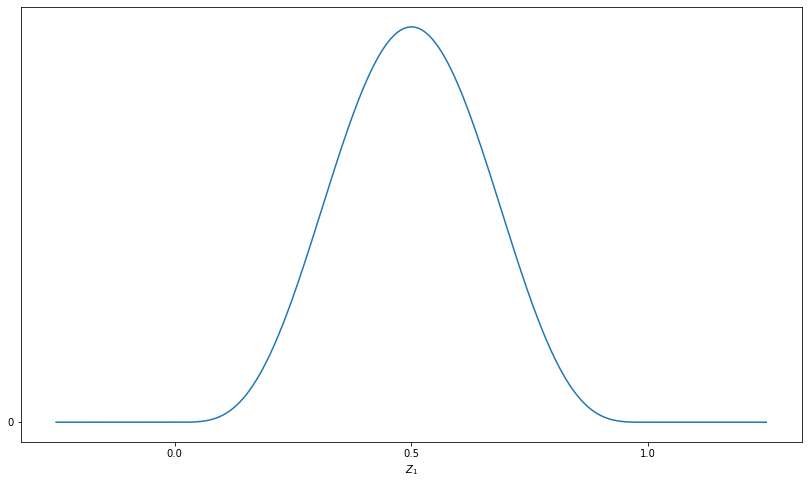
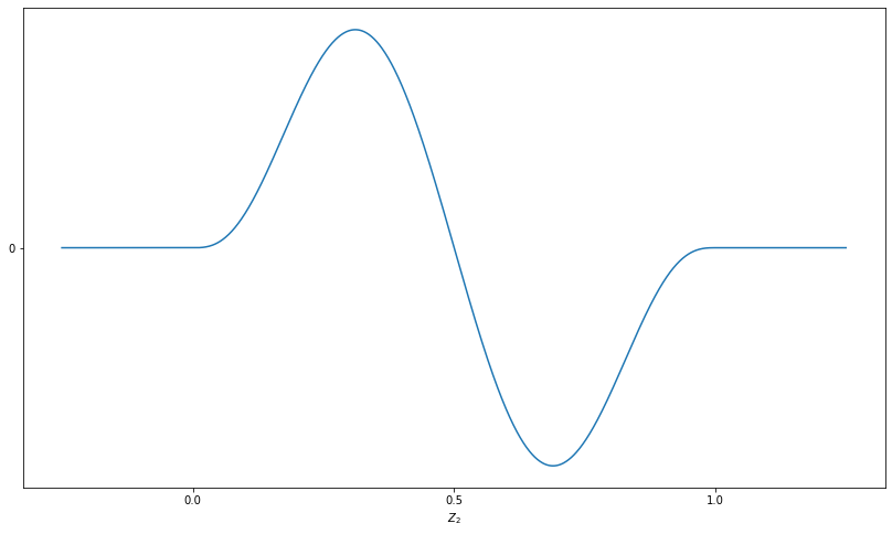
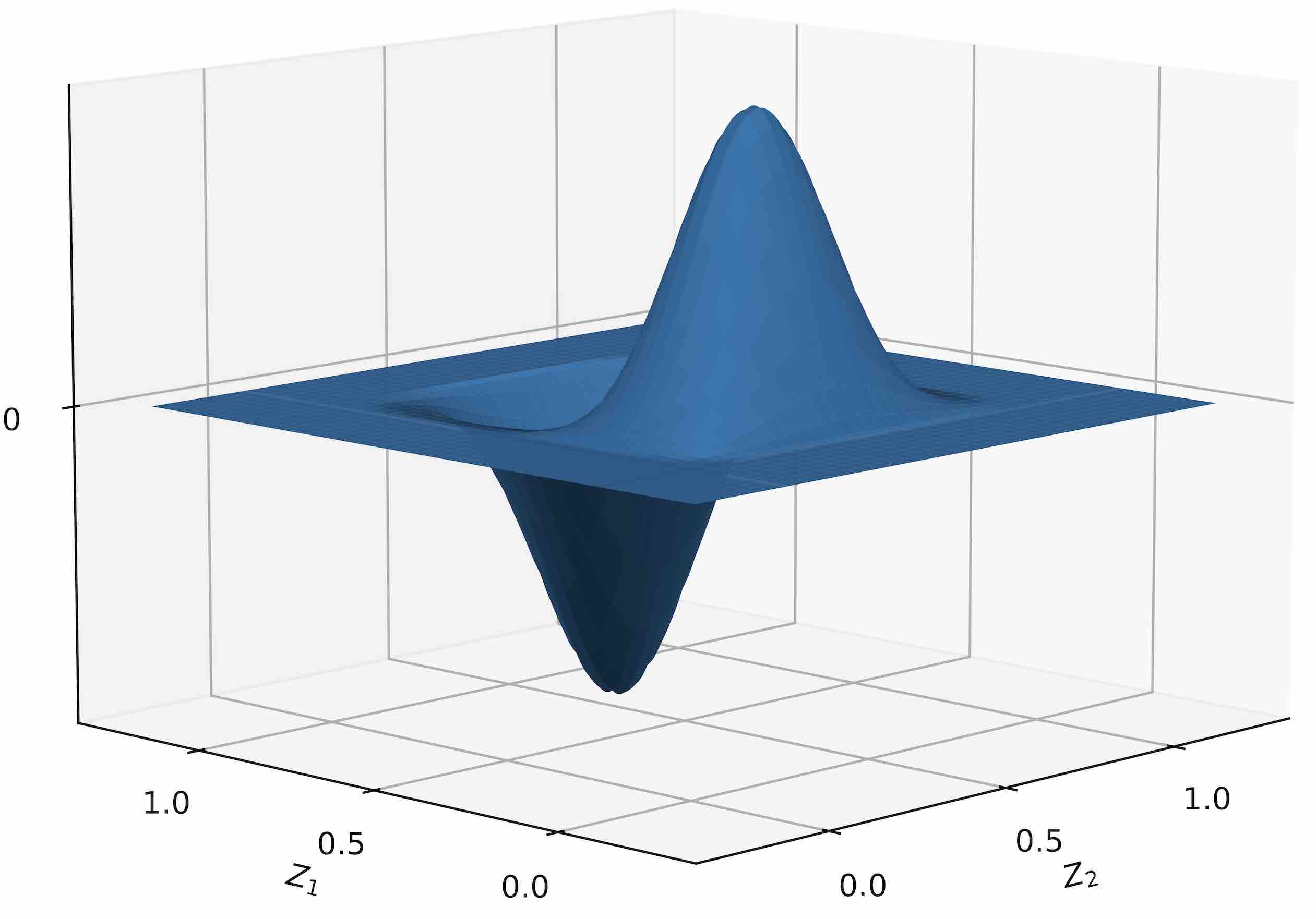
where denotes the largest integer less than or equal to . Figure 1 shows an illustration of and related functions. For a positive integer , with as , let , for , and . For a multi-index and , define as
where is a small enough constant described below. Then, it is easy to check that is a one-to-one function from onto itself, and for large enough .
Let be a uniform random variable on . Then, by the change of variables formula, the Lebesgue density of is given as
for , where denotes the derivative of . Here, is implicitly defined.
We first find an upper bound of for , where is the Kullback–Leibler divergence. Since and is bounded from above and below for small enough , where , we have
Since the ratio is bounded from above and below, we can use a well-known inequality , where denotes the Hellinger distance; see Lemma B.2 of Ghosal & van der Vaart [19]. Since , we have
Next, we derive a lower bound for . Suppose that for some . Then, the excess mass of over on is
In virtue of Corollary 1.16 in Villani [62], with the (unique) optimal transport plan between and , some portion of this excess mass must be transported at least the distance of , where constants and can be chosen so that they depend only on and . Hence, for some constant ,
where denotes the Hamming distance between and .
With the Hamming distance on , it is well-known (e.g. see page 124 of Wainwright [64]) that there is a -packing of whose cardinality is at least . Let be the convolution of and . Then, by Lemma B.11 of Ghosal & van der Vaart [19]. By the Fano’s method (Proposition 15.12 of Wainwright [64]), we have
If and is small enough, we have the desired result. ∎