Kyunghoon Ban
Rochester Institution of Technology
Rochester, NY
kban@saunders.rit.edu and Désiré Kédagni
UNC-Chapel Hill
Chapel Hill, NC
dkedagni@unc.edu

rdid and rdidstag: Stata commands for robust difference-in-differences

Ban and Kédagni

Abstract

This article provides a Stata package for the implementation of the robust difference-in-differences (RDID) method developed in Ban and Kédagni (2023). It contains three main commands: rdid, rdid_dy, rdidstag, which we describe in the introduction and the main text. We illustrate these commands through simulations and empirical examples.

keywords:

st0001, rdid, rdid_dy, rdidstag, robust DID

1 Introduction

In this article, we present the rdid, rdid_dy, rdidstag commands for estimation and inference on robust difference-in-differences (DID) bounds as developed by Ban and Kédagni (2023). These commands, summarized in Table 1, allows one to analyze the average treatment effects on the treated (ATT) under the canonical $2\times 2$ DID setting where observational data consist of two different groups (a treatment group and a control group) and two time periods (pre-treatment and post-treatment) as well as the staggered adoption design where there are multiple cohorts with different timings in the treatment adoption.

Table 1: Robust DID commands.

Command	Description
rdid	Estimates robust DID bounds on the ATT under the canonical $2\times 2$ DID setting.
rdid_dy	Estimates robust DID bounds on the ATTs for each of post-treatment periods under the canonical $2\times 2$ DID setting.
rdidstag	Estimates robust bounds on the cohort-time ATTs under the staggered adoption design.

Our article contributes to the expanding suite of publicly available software within the DID design community, including Villa (2016), Houngbedji (2016), de Chaisemartin et al. (2019), Rios-Avila et al. (2022, 2023), among others. Specifically, our software is more closely aligned with research exploring alternative identifying assumptions within the DID framework; for instance, Mora and Reggio (2015) examines DID estimations under alternative assumptions and assesses their robustness, while Bravo et al. (2022) discusses methods to bound post-treatment parallel trends (PT) violations using pre-treatment PT violations.

The rest of this article is structured as follows. In section 2, we recap the underlying frameworks of the robust DID bounds by Ban and Kédagni (2023). In sections 3, 4, and 5, we describe the rdid, rdid_dy, rdidstag commands, respectively. In section 6, we illustrate the performance of each command through a series of Monte Carlo simulations.

2 Framework and methodology

Consider the following potential outcome model:

\displaystyle Y_{t}

\displaystyle=

\displaystyle Y_{t}(1)D+Y_{t}(0)(1-D)

(1)

where $(Y_{t},D)$ , $t\in\mathcal{T}_{0}\cup\{1\}$ represents the observed data, while the vector $(Y_{1}(0),Y_{1}(1))$ is latent. The variables $Y_{t_{0}},Y_{1}\in\mathcal{Y}$ are respectively the observed outcomes in the baseline period $t_{0}\in\mathcal{T}_{0}$ and the follow-up period 1, while $D\in\left\{0,1\right\}$ is the observed treatment that occurred between periods 0 and 1, $Y_{1}(0)$ and $Y_{1}(1)$ are the potential outcomes that would have been observed in period 1 had the treatment $D$ been externally set to 0 and 1, respectively. $\mathcal{T}_{0}$ denotes the set of all pre-treatment periods. Model (1) assumes that there is no anticipatory effect of the treatment, so that $Y_{t_{0}}(1)=Y_{t_{0}}(0)$ for all baseline periods $t_{0}\in\mathcal{T}_{0}$ .

The standard DID estimand is defined as the difference between the OLS estimand in period 1 and the selection bias in period 0:

\theta_{DID}\equiv\theta_{OLS}-SB_{0}

where $\theta_{OLS}$ is the coefficient of a regression of $Y_{1}$ on the binary $D$ ,

\theta_{OLS}=\mathbb{E}[Y_{1}|D=1]-\mathbb{E}[Y_{1}|D=0],

and $SB_{t}$ is the selection bias in period $t$ ,

\displaystyle SB_{t}

\displaystyle=\mathbb{E}[Y_{t}(0)|D=1]-\mathbb{E}[Y_{t}(0)|D=0],

for $t\in\mathcal{T}_{0}\cup\{1\}$ . Recall that $SB_{0}$ is identified with the no anticipatory effect but $SB_{1}$ is an unobserved counterfactual.

Note that the average treatment effect on the treated (ATT),

ATT\equiv\mathbb{E}[Y_{1}(1)-Y_{1}(0)|D=1],

is identified by $\theta_{DID}$ under the parallel trend (PT) assumption,

\mathbb{E}[Y_{1}(0)-Y_{0}(0)|D=1]=\mathbb{E}[Y_{1}(0)-Y_{0}(0)|D=0],

or $SB_{1}=SB_{0}$ (bias stability).

Hence, the identification of ATT can be re-framed as imputing the counterfactual selection bias $SB_{1}$ . This observation inspires us to introduce a robust version of the DID estimand.

Define the baseline information set $\mathcal{I}_{0}\equiv\left\{(t_{0},x_{t_{0}}):x_{t_{0}}\in\mathcal{X}_{t_{0}},t_{0}\in\mathcal{T}_{0}\right\}$ , where $\mathcal{X}_{t_{0}}$ is the support of a baseline covariate $X_{t_{0}}$ in period $t_{0}$ , and $\mathcal{T}_{0}$ is the set of pre-treatment periods. For simplicity, suppose there are no baseline covariates so that $\mathcal{I}_{0}=\mathcal{T}_{0}$ .

Definition 1

Given the baseline information set $\mathcal{I}_{0}=\mathcal{T}_{0}$ , we define the robust difference-in-differences (RDID) estimand as

\displaystyle\theta_{RDID}\equiv\theta_{OLS}-\operatorname{Conv}\big{(}SB(\mathcal{T}_{0})\big{)},

(2)

where $\operatorname{Conv}(A)$ is the convex hull of a generic set $A$ , $SB$ is a function defined as

	$\displaystyle SB\colon\quad\mathcal{I}_{0}$	$\displaystyle\to$	$\displaystyle\mathbbm{R},$
	$\displaystyle\iota_{0}$	$\displaystyle\mapsto$	$\displaystyle SB(t_{0})=SB_{t_{0}},$

and $SB(\mathcal{T}_{0})$ is the image of the information set $\mathcal{I}_{0}=\mathcal{T}_{0}$ through the function $SB$ .

When baseline covariates exists, we define the function $SB$ as

\begin{array}[]{llcl}SB\colon&\mathcal{I}_{0}&\to&\mathbbm{R},\\ &\iota_{0}\equiv(t_{0},x_{t_{0}})&\mapsto&SB(\iota_{0})\equiv\mathbb{E}[Y_{t_{0}}|D=1,X_{t_{0}}=x_{t_{0}}]-\mathbb{E}[Y_{t_{0}}|D=0,X_{t_{0}}=x_{t_{0}}].\end{array}

In the above definition, if there is only one element in the information, i.e., $\mathcal{I}_{0}=\mathcal{T}_{0}=\{0\}$ , then $\operatorname{Conv}\big{(}SB(\mathcal{T}_{0})\big{)}=SB_{0}$ , and the robust DID estimand is the same as the standard DID estimand.

2.1 Bias set stability

Let us first consider the simple case with no covariates in the model.

Assumption 1 (Bias set stability)

\displaystyle SB_{1}\in\left[\inf_{\iota_{0}\in\mathcal{I}_{0}}SB(\iota_{0}),\sup_{\iota_{0}\in\mathcal{I}_{0}}SB(\iota_{0})\right]\equiv\Delta_{SB(\mathcal{I}_{0})},

where $SB(\iota_{0})$ is defined above.

Assumption 1 is weaker than the standard “parallel/common trends” assumption. Indeed, if $\mathcal{I}_{0}$ is the singleton of a single baseline information $I_{0}=\{0\}$ , then Assumption 1 is equivalent to $SB_{1}=SB_{0},$ which is equivalent to the parallel trends assumption.

Under Assumption 1, robust DID estimand yields the following bounds on the ATT.¹¹1Note that the RDID can be generalized by using other correspondences $f(SB(\mathcal{I}_{0}))$ than $\operatorname{Conv}(SB(\mathcal{I}_{0}))$ associated with other assumptions (Ban and Kédagni, 2023).

Proposition 1

Suppose that model (1) along with Assumption 1 holds. Then, the following bounds hold for the ATT:

\displaystyle ATT\in\left[\theta_{OLS}-\sup_{\iota_{0}\in\mathcal{I}_{0}}SB(\iota_{0}),\theta_{OLS}-\inf_{\iota_{0}\in\mathcal{I}_{0}}SB(\iota_{0})\right]\equiv\Theta_{I}.

These bounds are sharp, and $\Theta_{I}$ is the identified set for the ATT.

The bounds in Proposition 1 are never empty, as they always contain the standard DID estimand under the parallel trends assumption. However, they may not contain the OLS estimand in period 1, $\theta_{OLS}$ , as 0 may not lie within the set $\Delta_{SB(\mathcal{I}_{0})}$ . If all pre-treatment periods selection biases are equal, i.e., $SB(\iota_{0})=SB_{0}$ for all $\iota_{0}$ , then our bounds collapse to a point, the standard DID estimand. In case the information set $\mathcal{I}_{0}$ is the set of pre-treatment periods, the above bounds are robust to violations of PT that can be captured in the pre-treatment periods.

2.2 PO-RDID: Best predictor of $SB_{1}$ based on a loss function

Consider a random variable $I_{0}$ representing the baseline information with a distribution $\mu_{I_{0}}$ . Provided $\mu_{I_{0}}$ is known, we are going to assume that the decision maker will choose the selection bias $SB_{1}$ in such a way that a loss function is minimized. By plugging such an optimal selection bias $SB_{1}$ into the definition of the robust DID, we obtain what we call a policy-oriented robust difference-in-differences (PO-RDID) estimand. This estimand may not have a causal interpretation, but it may help the policy-maker in her decision making process.

Assumption 2

Let $\mathcal{L}(b;SB(\mathcal{I}_{0}),\mu_{I_{0}})$ be the decision maker’s loss function when she observes a (random) baseline information $I_{0}$ and chooses a selection bias $b$ . The decision maker chooses $b$ (or $SB_{1}$ ) to minimize the loss $\mathcal{L}(b)$ : $SB_{1}^{opt}=\arg\min_{b}\mathcal{L}(b;SB(\mathcal{I}_{0}),\mu_{I_{0}})$ .

In this paper, we consider the class of $p$ -norm losses defined as:

\mathcal{L}_{p}(b;SB(\mathcal{I}_{0}),\mu_{I_{0}})=\left(\mathbb{E}_{\mu_{I_{0}}}\left[|b-SB(I_{0})|^{p}\right]\right)^{1/p},

where $1\leq p\leq\infty$ . We are going to derive the optimal selection bias $SB_{1}^{opt}$ for $p\in\left\{1,2,\infty\right\}$ . We consider those special loss functions because the solutions to the optimization problem have closed-form expressions. Other loss functions can also be considered.

The command rdid with an option rdidtype(1) can be used, and the distribution of $SB_{0}(I_{0})$ is estimated by the proportion of observations at each level of $I_{0}$ .

$L1$ loss: Mean absolute error (MAE)

Note that $\mathcal{L}_{1}(b;SB(\mathcal{I}_{0}),\mu_{I_{0}})=\mathbb{E}_{\mu_{I_{0}}}\left[|b-SB(I_{0})|\right]$ . Given this $L1$ loss function, under Assumption 2, the decision maker solves the following optimization problem:

\displaystyle\min_{SB_{1}}\mathbb{E}_{\mu_{I_{0}}}\left[|SB_{1}-SB(I_{0})|\right].

The optimal decision is to set the selection $SB_{1}$ to be equal to the median selection bias in the baseline period, i.e., $SB_{1}^{opt}=Med_{\mu_{I_{0}}}\big{(}SB(I_{0})\big{)}$ . In such a case, the policy-oriented robust DID estimand is given by

\theta_{PO-RDID}^{\mathcal{L}_{1}}=\theta_{OLS}-Med_{\mu_{I_{0}}}\big{(}SB(I_{0})\big{)}.

$L2$ loss: Root mean square error (RMSE)

We have $\mathcal{L}_{2}(b;SB(\mathcal{I}_{0}),\mu_{I_{0}})=\left(\mathbb{E}_{\mu_{I_{0}}}\left[|b-SB_{0}(I_{0})|^{2}\right]\right)^{1/2}$ , and minimizing the RMSE is equivalent to minimizing the mean square error (MSE). Therefore, under Assumption 2, the decision maker solves the following optimization problem:

\displaystyle\min_{SB_{1}}\mathbb{E}_{\mu_{I_{0}}}\left[\left(SB_{1}-SB(I_{0})\right)^{2}\right].

This yields an optimal decision for the selection $SB_{1}$ to be set equal to the average selection bias in the baseline period, i.e., $SB_{1}^{opt}=\mathbb{E}_{\mu_{I_{0}}}[SB(I_{0})]$ . Hence, we have

\theta_{PO-RDID}^{\mathcal{L}_{2}}=\theta_{OLS}-\mathbb{E}_{\mu_{I_{0}}}[SB(I_{0})].

$L\infty$ loss: Maximal regret

Note that

	$\displaystyle\mathcal{L}_{\infty}(b;SB(\mathcal{I}_{0}),\mu_{I_{0}})$	$\displaystyle=\text{ess}\sup\|b-SB(I_{0})\|,$
		$\displaystyle=\inf\Big{\{}M\geq 0:\mathbbm{P}_{\mu_{I_{0}}}\big{(}\|b-SB(I_{0})\|\leq M\big{)}=1\Big{\}}.$

This optimization problem with the $L\infty$ loss is equivalent to a minimax criterion, and yields the mid-point of the bounds on $SB_{1}$ stated in Assumption 1. Hence, the PO-RDID estimand is given by

\theta_{PO-RDID}^{\mathcal{L}_{\infty}}=\theta_{OLS}-\frac{1}{2}\bigg{(}\inf_{\iota_{0}\in\mathcal{I}_{0}}SB(\iota_{0})+\sup_{\iota_{0}\in\mathcal{I}_{0}}SB(\iota_{0})\bigg{)}.

Note that in all cases, if the information in the baseline period is a singleton, then the optimal $SB_{1}^{opt}$ is the selection bias in the baseline period $SB_{0}$ , which is equivalent to the parallel trends assumption. Unlike the PO-RDID estimand obtained from $L1$ and $L2$ loss functions, that obtained from the $L\infty$ loss function does not require the knowledge of the distribution $\mu_{I_{0}}$ of the information $I_{0}$ but only its support and is easy to compute. However, when the distribution of $SB(I_{0})$ is uniform over $\left[\inf_{\iota_{0}\in\mathcal{I}_{0}}SB(\iota_{0}),\sup_{\iota_{0}\in\mathcal{I}_{0}}SB(\iota_{0})\right]$ , then the optimal selection bias $SB_{1}^{opt}$ is the same in all three cases.

2.3 Forecasting $SB_{1}$ when the baseline information is ordered

Suppose that the baseline information set $\mathcal{I}_{0}$ is ordered (e.g., a set of multiple pre-treatment periods $\mathcal{I}_{0}=\{-T_{0},-T_{0}+1,\ldots,-1,0\}$ or a continuous baseline covariate $X_{0}$ like age). We can regress $SB(I_{0})$ on $\{I_{0},I_{0}^{2},\ldots\}$ and use this regression to predict $SB_{1}$ .

For instance, if $\mathcal{I}_{0}=\{-T_{0},-T_{0}+1,\ldots,-1,0\}$ and the selection bias $SB(I_{0})$ is increasing over time, Assumption 1 may not hold. The researcher could instead use this increasing trend information about the selection bias to forcast the next period selection bias $\widehat{SB}_{1}$ .

The command rdid with an option rdidtype(2) can be used for a linear predicition model, and an option peval(#) can be used to specify the evaluation point of the prediction.

2.4 Identification with multiple periods

We generalize our analysis to a setting where the treatment receipt occurs at multiple periods. We consider the following multiple treatment periods potential outcome model:

\displaystyle Y_{t}

\displaystyle=

\displaystyle\sum_{(d_{1},\ldots,d_{T})\in\{0,1\}^{T}}Y_{t}(0,d_{1},\ldots,d_{T})\mathbbm{1}\{D_{0}=0,D_{1}=d_{1},\ldots,D_{T}=d_{T}\},

(3)

for $t\in\mathcal{T}_{0}\cup\{1,\ldots,T\}$ , where $Y_{t}$ denotes the observed outcome in period $t$ , $D_{t}$ is the observed treatment status in period $t$ with $D_{0}=0$ by definition, while $Y_{t}(0,d_{1},\ldots,d_{T})$ is the potential outcome when the treatment path $(D_{0},D_{1},\ldots,D_{T})$ is externally set to $(0,d_{1},\ldots,d_{T})$ .²²2See Robins (1986, 1987), and Han (2021) for a similar definition of the potential outcome model. Under the no-anticipation assumption, we have $Y_{t_{0}}(0,d_{1},\ldots,d_{T})=Y_{t_{0}}(0)$ for all $(d_{1},\ldots,d_{T})\in\{0,1\}^{T}$ and $t_{0}\in\mathcal{T}_{0}$ . That is, we assume that individuals do not anticipate any effects of the treatment before it occurs for the first time in $t=1$ . However, we allow the individuals to anticipate the effects of the treatment for the rest of the period. This assumption is less restrictive than the commonly used no-anticipatory effects assumption.

In the above framework, the parameter of interest is the average treatment effect in period $t$ on the treated group following the path $\bm{d}^{0}\equiv(0,d_{1}^{0},\ldots,d_{T}^{0})$ to $\bm{d}^{1}\equiv(0,d_{1}^{1},\ldots,d_{T}^{1})$ , which is defined as:

	$\displaystyle ATT_{t}[\bm{d}^{0}\rightarrow\bm{d}^{1}]$
	$\displaystyle\qquad\qquad\equiv\mathbb{E}\left[Y_{t}(\bm{d}^{1})-Y_{t}(\bm{d}^{0})\|(D_{0},D_{1},\ldots,D_{T})=\bm{d}^{1}\right].$

Similarly to what we have in the one post-treatment setting, we can write the difference-in-means estimand $(\theta_{DIM}^{t})$ between the two groups $\bm{d}^{0}$ and $\bm{d}^{1}$ in period $t$ as:

	$\displaystyle\theta_{DIM}^{t}[\bm{d}^{0}\rightarrow\bm{d}^{1}]$	$\displaystyle\equiv\mathbb{E}\left[Y_{t}\|(D_{0},D_{1},\ldots,D_{T})=\bm{d}^{1}\right]-\mathbb{E}\left[Y_{t}\|(D_{0},D_{1},\ldots,D_{T})=\bm{d}^{0}\right]$
		$\displaystyle=ATT_{t}[\bm{d}^{0}\rightarrow\bm{d}^{1}]+SB_{t}[\bm{d}^{0}\rightarrow\bm{d}^{1}],$

where $SB_{t}[\bm{d}^{0}\rightarrow\bm{d}^{1}]\equiv\mathbb{E}\left[Y_{t}(\bm{d}^{0})|(D_{0},D_{1},\ldots,D_{T})=\bm{d}^{1}\right]-\mathbb{E}\left[Y_{t}(\bm{d}^{0})|(D_{0},D_{1},\ldots,D_{T})=\bm{d}^{0}\right]$ . We extend Assumption 1 to the current setting.

Assumption 3 (Extended bias set stability)

For each $t$ ,

	$\displaystyle SB_{t}[\bm{d}^{0}\rightarrow\bm{d}^{1}]$	$\displaystyle\in\left[\inf_{t_{0}\in\mathcal{T}_{0}}SB_{t_{0}}[\bm{d}^{0}\rightarrow\bm{d}^{1}],\sup_{t_{0}\in\mathcal{T}_{0}}SB_{t_{0}}[\bm{d}^{0}\rightarrow\bm{d}^{1}]\right]$
		$\displaystyle\equiv\Delta_{SB(\mathcal{T}_{0})}[\bm{d}^{0}\rightarrow\bm{d}^{1}],$

where $SB_{t_{0}}[\bm{d}^{0}\rightarrow\bm{d}^{1}]\equiv\mathbb{E}[Y_{t_{0}}(0)|(D_{0},D_{1},\ldots,D_{T})=\bm{d}^{1}]-\mathbb{E}[Y_{t_{0}}(0)|(D_{0},D_{1},\ldots,D_{T})=\bm{d}^{0}]$ is the baseline selection bias with respect to the treatment status in period $t_{0}\in\mathcal{T}_{0}$ when the information set $\mathcal{I}_{0}$ is equal to $\mathcal{T}_{0}$ .

Assumption 3 is a generalization of Assumption 1, and we have the following identification results for $ATT_{t}$ with different treatment paths.

Proposition 2

Suppose that model (3) along with Assumption 3 holds. Then, the following bounds are valid for $ATT_{t}$ :

	$\displaystyle ATT_{t}[\bm{d}^{0}\rightarrow\bm{d}^{1}]$
	$\displaystyle\qquad\in\left[\theta_{DIM}^{t}[\bm{d}^{0}\rightarrow\bm{d}^{1}]-\sup_{t_{0}\in\mathcal{T}_{0}}SB_{t_{0}}[\bm{d}^{0}\rightarrow\bm{d}^{1}],\theta_{DIM}^{t}[\bm{d}^{0}\rightarrow\bm{d}^{1}]-\inf_{t_{0}\in\mathcal{T}_{0}}SB_{t_{0}}[\bm{d}^{0}\rightarrow\bm{d}^{1}]\right],$
	$\displaystyle\qquad\equiv\Theta_{I}^{t}[\bm{d}^{0}\rightarrow\bm{d}^{1}].$

These bounds are sharp, and $\Theta_{I}^{t}[\bm{d}^{0}\rightarrow\bm{d}^{1}]$ is the identified set for $ATT_{t}[\bm{d}^{0}\rightarrow\bm{d}^{1}]$ .

In a staggered design setting, the average treatment effect in period $t$ on units who are treated for the first time in period $g$ could be an interesting parameter, as considered in Callaway and Sant’Anna (2021):

ATT(g,t)\equiv ATT_{t}[(0,\ldots,0,d_{g}=0,0,\ldots,0)\rightarrow(0,\ldots,0,d_{g}=1,1,\ldots,1)].

By defining $G$ as

G=\left\{\begin{array}[]{ccl}g&\mathrm{if}&(D_{0},D_{1},\ldots,D_{T})=(0,\ldots,0,d_{g}=1,1,\ldots,1)\\ \infty&\mathrm{if}&(D_{0},D_{1},\ldots,D_{T})=(0,\ldots,0)\end{array}\right.,

where $G=\infty$ denotes the never-treated cohort as our control group, we can write

	$\displaystyle\theta^{t}_{DIM}[\infty\rightarrow g]$	$\displaystyle\equiv\theta^{t}_{DIM}[(0,\ldots,0)\rightarrow(0,\ldots,0,d_{g}=1,1,\ldots,1)]$
		$\displaystyle=\mathbb{E}[Y_{t}\|G=g]-\mathbb{E}[Y_{t}\|G=\infty]$
	$\displaystyle SB_{t}[\infty\rightarrow g]$	$\displaystyle\equiv SB_{t}[(0,\ldots,0)\rightarrow(0,\ldots,0,d_{g}=1,1,\ldots,1)]$
		$\displaystyle=\mathbb{E}[Y_{t}(g)\|G=g]-\mathbb{E}[Y_{t}(\infty)\|G=\infty],$

for $t\in\mathcal{T}_{0}\cup\{1,\ldots,T\}$ , by abusing the notations of $g$ and $\infty$ for paths.

Hence, Assumption 3 can be re-written as

	$\displaystyle SB_{t}[\infty\rightarrow g]$	$\displaystyle\in\left[\inf_{t_{0}\in\mathcal{T}_{0}}SB_{t_{0}}[\infty\rightarrow g],\sup_{t_{0}\in\mathcal{T}_{0}}SB_{t_{0}}[\infty\rightarrow g]\right]$
		$\displaystyle\equiv\Delta_{SB(\mathcal{T}_{0})}[\infty\rightarrow g],$

for each $t\in\{1,\ldots,T\}$ , and $SB_{t_{0}}[\infty\rightarrow g]\equiv\mathbb{E}[Y_{t_{0}}(0)|G=g]-\mathbb{E}[Y_{t_{0}}(0)|G=\infty]$ for $t\in\mathcal{T}_{0}$ . Thus, we have

	$\displaystyle ATT(g,t)$	$\displaystyle\in\left[\theta_{DIM}^{t}[\infty\rightarrow g]-\sup_{t_{0}\in\mathcal{T}_{0}}SB_{t_{0}}[\infty\rightarrow g],\theta_{DIM}^{t}[\infty\rightarrow g]-\inf_{t_{0}\in\mathcal{T}_{0}}SB_{t_{0}}[\infty\rightarrow g]\right].$
		$\displaystyle\equiv\Theta(g,t)$

3 The rdid command

3.1 Syntax

The rdid command estimates bounds on the ATT under the assumptions discussed above. The syntax for the rdid command is

rdid depvar $\bigl{[}\,$ indepvars $\,\bigr{]}$ $\bigl{[}$ if $\bigr{]}$ $\bigl{[}$ in $\bigr{]}$ , treatname(varname) postname(varname) infoname(varname) $\bigl{[}$ rdidtype(#) peval(#) level(#) figure brep(#) clustername(varname) $\bigr{]}$

3.2 Options

treatname(varname) specifies the variable name of the treatment indicator. treatname() is required.

postname(varname) specifies the variable name of the post-treatment period indicator. postname() is required.

infoname(varname) specifies the variable name of the information index. infoname() is required.

rdidtype(#) specifies the type of RDID estimator; 0 for the simple RDID, 1 for the policy-oriented (PO) RDID, and 2 for the RDID with linear predictions. The default is rdidtype(0).

peval(#) specifies the evaluation point for the RDID with linear predictions. The default is the mean value of infoname(varname) in the post-treatment period. This option is ignored when rdidtype(#) is not equal to 2.

level(#) specifies the confidence level, as a percentage, for confidence intervals (CIs). The default is level(95). Three different CIs are provided with rdidtype(0); 1) CI for the bounds (Ye et al., 2023), 2) CI for the ATT (Ye et al., 2023), and 3) CI for the bounds (union bounds). Bootstrapped CIs are provided with rdidtype(1) and rdidtype(2).

When figure(string) is specified, rdid saves a scatter plot of estimated selection biases and the information index in the pre-treatment periods as figure(string).png.

brep(#) specifies the number of bootstrap replicates. The default is brep(500).

clustername(varname) specifies the variable name that identifies resampling clusters in bootstrapping.

3.3 Stored results

rdid stores the following in e(). When indepvars is specified, $\tau^{DR}$ is estimated using post-treatment periods (see Ban and Kédagni, 2023) and stored in e(DR). Otherwise, $\theta_{OLS}$ is estimated and stored in e(OLS). Also, stored scalars depend on rdidtype(#) specification (referred as ‘type’ below). In the following, LB (UB) stands for lower bound (upper bound).

Scalars (common)
e(DR)	$\widehat{\tau}^{DR}$ estimate	e(OLS)	$\widehat{\theta}_{OLS}$ estimate
e(N)	number of observations
Scalars (type=0)
e(SB_LB)	LB of $\widehat{\Delta}_{SB(\mathcal{I}_{0})}$	e(SB_UB)	UB of $\widehat{\Delta}_{SB(\mathcal{I}_{0})}$
e(RDID_LB)	LB of $\widehat{\Theta}_{I}$	e(RDID_UB)	UB of $\widehat{\Theta}_{I}$
e(CI1_LB)	LB of CI-1	e(CI1_UB)	UB of CI-1
e(CI2_LB)	LB of CI-2	e(CI2_UB)	UB of CI-2
e(CI3_LB)	LB of CI-3	e(CI3_UB)	UB of CI-3
Scalars (type=1)
e(L1_CI_LB)	LB of CI for $\widehat{\theta}_{PO-RDID}^{\mathcal{L}_{1}}$	e(L1_CI_LB)	UB of CI for $\widehat{\theta}_{PO-RDID}^{\mathcal{L}_{1}}$
e(L2_CI_LB)	LB of CI for $\widehat{\theta}_{PO-RDID}^{\mathcal{L}_{2}}$	e(L2_CI_LB)	UB of CI for $\widehat{\theta}_{PO-RDID}^{\mathcal{L}_{2}}$
e(Linf_CI_LB)	LB of CI for $\widehat{\theta}_{PO-RDID}^{\mathcal{L}_{\infty}}$	e(Linf_CI_LB)	UB of CI for $\widehat{\theta}_{PO-RDID}^{\mathcal{L}_{\infty}}$
e(L1_PE)	$\widehat{\theta}_{PO-RDID}^{\mathcal{L}_{1}}$ estimate	e(L2_PE)	$\widehat{\theta}_{PO-RDID}^{\mathcal{L}_{2}}$ estimate
e(Linf_PE)	$\widehat{\theta}_{PO-RDID}^{\mathcal{L}_{\infty}}$ estimate
Scalars (type=2)
e(SB_hat)	$\widehat{SB}_{1}$ estimate	e(proj_PE)	$\widehat{\theta}_{RDID}$ estimate
e(CI_LB)	LB of CI for $\widehat{\theta}_{RDID}$	e(CI_UB)	UB of CI for $\widehat{\theta}_{RDID}$
Macros
e(cmd)	rdid	e(indep)	name of independent variable
e(depvar)	name of dependent variable(s)	e(clustvar)	name of cluster variable
e(level)	confidence level
Matrices
e(results)	displayed summary matrix

4 The rdid_dy command

4.1 Syntax

The rdid_dy command is a wrapper command that implements RDID estimation separately for each levels of a time variable in the post-treatment period and collects the results. The syntax for the rdid_dy command is

rdid_dy depvar $\bigl{[}\,$ indepvars $\,\bigr{]}$ $\bigl{[}$ if $\bigr{]}$ $\bigl{[}$ in $\bigr{]}$ , treatname(varname) postname(varname) infoname(varname) tname(varname) $\bigl{[}$ rdidtype(#) peval(#) level(#) figure(string) brep(#) clustername(varname) citype(#) losstype(#) $\bigr{]}$

4.2 Options

tname(varname) specifies the variable name for the time. tname() is required.

peval(#) specifies the evaluation point for the RDID with linear predictions. The default is the mean value of infoname(varname) in the post-treatment period. In particular, if infoname(varname) is the same as tname(varname), each RDID estimate is obtained using each level of tname(varname) as the evaluation point. This option is ignored when rdidtype(#) is not equal to 2.

When figure(string) is specified, rdid_dy saves line plots of RDID estimates and confidence intervals over the post-treatment periods as figure(string).png.

citype(varname) specifies the type of confidence intervals to collect for rdidtype(0); 1 yields CI for the RDID bounds (Ye et al., 2023), 2 yields CI for the ATT (Ye et al., 2023), and 3 yields CI for the RDID bounds (Union Bounds). The default is citype(1). This option is ignored when rdidtype(#) is not equal to 0.

losstype(#) specifies the type of loss function for rdidtype(1) (PO-RDID); 1 for $\mathcal{L}_{1}$ , 2 for $\mathcal{L}_{2}$ , and 0 for $\mathcal{L}_{\infty}$ . The default is losstype(1). This option is ignored when rdidtype(#) is not equal to 1.

4.3 Stored results

rdid_dy stores the following in e(). Stored scalars depend on rdidtype(#) specification; In the following, LB (UB) stands for lower bound (upper bound) and (t) denotes each level of tname(varname).

Scalars
e(N)	number of observations	e(RDID_PE_(t))	$\widehat{\theta}_{RDID}$ estimate for (t)
e(RDID_LB_(t))	LB of $\widehat{\Theta}_{I}$ for (t)	e(RDID_UB_(t))	UB of $\widehat{\Theta}_{I}$ for (t)
e(RDID_LB_(t))	LB of CI for (t)	e(RDID_UB_(t))	LB of CI for (t)
Macros
e(cmd)	rdid_dy	e(indep)	name of independent
			variable
e(depvar)	name of dependent	e(clustvar)	name of cluster variable
	variable(s)
e(level)	confidence level
Matrices
e(results)	displayed summary matrix

5 The rdidstag command

5.1 Syntax

The rdidstag command estimates bounds on the ATT over time for different cohorts in the staggered adoption design under the assumptions discussed above. The syntax for the rdidstag command is

rdidstag depvar $\bigl{[}\,$ indepvars $\,\bigr{]}$ $\bigl{[}$ if $\bigr{]}$ $\bigl{[}$ in $\bigr{]}$ , gname(varname) tname(varname) $\bigl{[}$ postname(varname) infoname(varname) level(#) figure clustername(varname) $\bigr{]}$

5.2 Options

gname(varname) specifies the variable name of the cohort index, $g\in\mathcal{G}$ , where $g=0$ is assigned for the never-treated group. gname() is required.

tname(varname) specifies the variable name of time index, $t$ . tname() is required.

postname(varname) specifies the variable name of the post-treatment period indicator. The default is using units with $t\geq\min(\mathcal{G}\setminus\{0\})$ as post-period units.

infoname(varname) specifies the variable name of the information index. The default is using pre-treatment periods; i.e., $\mathcal{I}_{0}=\{t\mid t<\min(\mathcal{G}\setminus\{0\})\}$ .

level(#) specifies the confidence level, as a percentage, for confidence intervals. The default is level(95).

When figure is specified, rdidstag saves line plots of RDID bounds and confidence intervals over the post-treatment periods for each $g\in\mathcal{G}$ as figure(string).png.

clustername(varname) specifies the variable name that identifies resampling clusters in bootstrapping.

5.3 Stored results

rdidstag stores the following in e(). In the following, LB (UB) stands for lower bound (upper bound). Also, (g) and (t) denote each level of gname(varname) and tname(varname), respectively.

Scalars
e(RDID_LB_(g)_(t))	LB of $\widehat{\Theta}(g,t)$	e(RDID_UB_(g)_(t))	UB of $\widehat{\Theta}(g,t)$
e(CI_LB_(g)_(t))	LB of CI for $\widehat{\Theta}(g,t)$	e(CI_UB_(g)_(t))	UB of CI for $\widehat{\Theta}(g,t)$
e(N)	number of observations
Macros
e(cmd)	rdidstag	e(indep)	name of independent
			variable
e(depvar)	name of dependent	e(clustvar)	name of cluster variable
	variable(s)
e(level)	confidence level
Matrices
e(results)	displayed summary matrix

6 Applications

We illustrate usages of rdid, rdid_dy, and rdidstag commands using two applications. We first demonstrate rdid and rdid_dy commands using an application of Cai (2016) in Section 6.1 and then rdidstag command using data from Dube et al. (2016) in Section 6.2.

6.1 Effects of insurance provision on tobacco production

Cai (2016) investigates the impact of insurance provision on tobacco production using a household-level panel dataset provided by the Rural Credit Cooperative (RCC), the main rural bank in China.

Using rdid command

In the following runs, the dependent variable is area_tob and the covariates are hhsize, educ_scale, and age, yielding the doubly-robust estimate (Ban and Kédagni, 2023). Also, treatment variable and the post-treatment period indicator is is treatment and policy2, respectively, and the information set is specified as pre-treatment periods by using year. We use 1,000 bootstrap replicates and cluster the standard errors using hhno. First, the following is yielding the RDID bounds with the three different confidence intervals.

. use "analysis.dta"

. drop if sector != 1
(20,519 observations deleted)

. rdid area_tob hhsize educ_scale age, treat(treatment) post(policy2) ///
>         info(year)  b(1000) cl(hhno)
 **** RDID Estimation version 1.8 ****
Y name: area_tob
D name: treatment
X name(s): hhsize educ_scale age

                                       
    Y: area_tob           LB        UB
                                       
           RDID       0.8086    0.9479
           CI_1       0.6203    1.1257
           CI_2       0.6235    1.1222
           CI_3       0.6187    1.1257
                                       
* RDID: Point estimates for RDID bounds
* CI_1: Confidence interval for the bounds (Ye et al.)
* CI_2: Confidence interval for the ATT (Ye et al.)
* CI_3: Confidence interval for the bounds (Union Bounds)

Second, by specifying the option rdidtype(1), we can have PO-RDID estimates and their confidence intervals under the three loss functions.

. rdid area_tob hhsize educ_scale age, treat(treatment) post(policy2) ///
>         info(year) rdidtype(1) b(1000) cl(hhno)
 **** RDID Estimation version 1.8 ****
Y name: area_tob
D name: treatment
X name(s): hhsize educ_scale age

                                           
    Y: area_tob         PE   CI_LB   CI_UB
                                           
             L1     0.8770  0.6732  1.0806
             L2     0.8778  0.6911  1.0753
           Linf     0.8783  0.6978  1.0710

Lastly, by specifying the option rdidtype(2), we can have an RDID estimate based on a linear prediction with an ordered information set, pre-treatment periods. The predicted value is evaluated at the mean of the post-treatment periods, 2005.5, with the option peval(2005.5).

. rdid area_tob hhsize educ_scale age, treat(treatment) post(policy2) ///
>         info(year) rdidtype(2) peval(2005.5) b(1000) cl(hhno)
 **** RDID Estimation version 1.8 ****
Y name: area_tob
D name: treatment
X name(s): hhsize educ_scale age

                                                           
                        PE   CI_LB   CI_UB  TAU_DR  SB_hat
                                                           
Y                  
       area_tob     0.7239  0.4760  0.9725  1.9154  1.1914

Using rdid_dy command

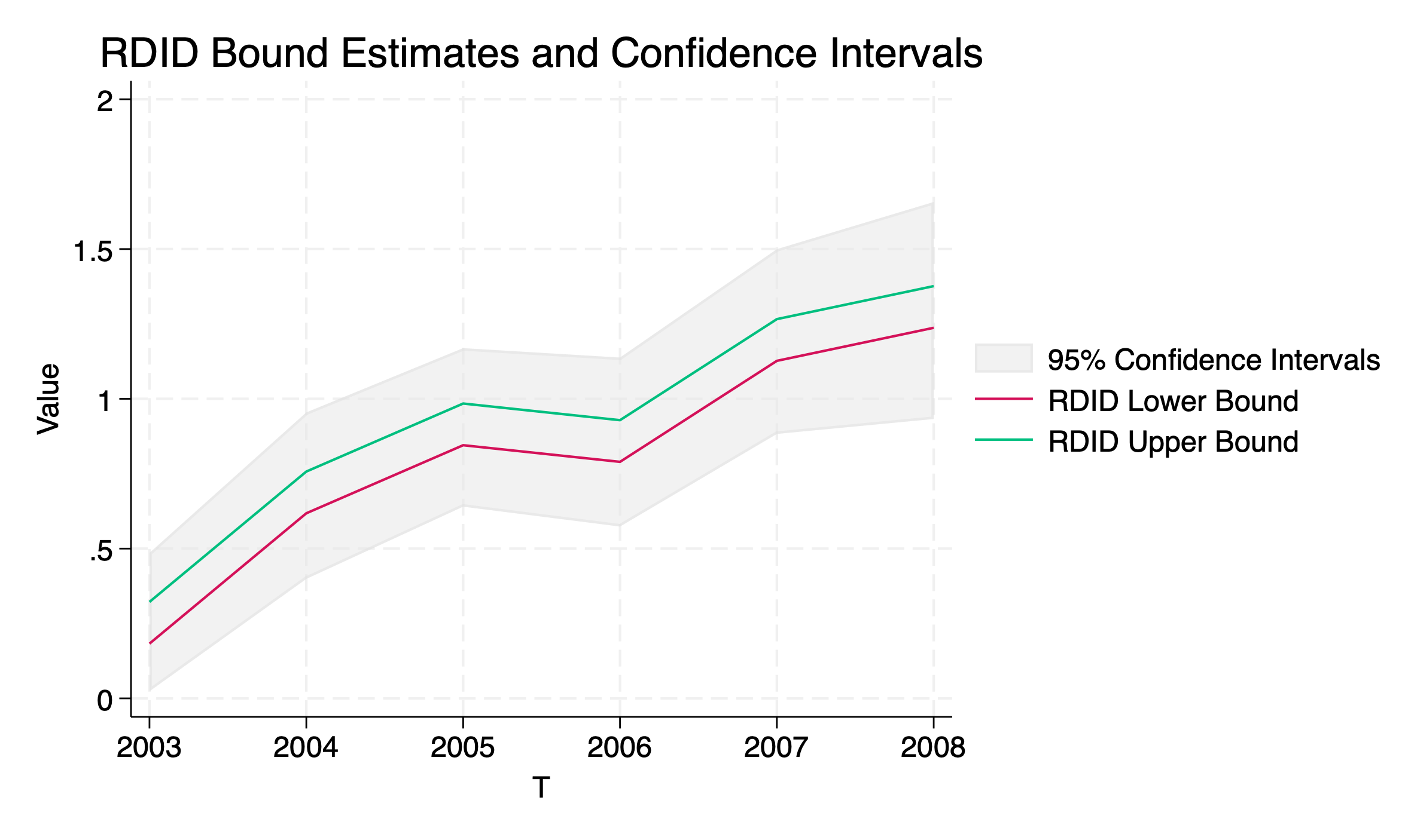
Recall that rdid_dy command is a wrapper command that implements RDID estimation separately for each levels of a time variable in the post-treatment period and collects the results. In the following runs, the same options are specified as before, but the option tname(year) is used to denote the variable for the post-treatment periods. Also, the following run produces Figure 1 that summarizes the output.

. use "analysis.dta"

. drop if sector != 1
(20,519 observations deleted)

. rdid_dy area_tob hhsize educ_scale age, treat(treatment) post(policy2) ///
>         info(year) tname(year) fig b(1000) cl(hhno)
file rdid_dy.png saved as PNG format

                                                           
        T: year      RDID_LB   RDID_UB     CI_LB     CI_UB
                                                           
           2003       0.1829    0.3221    0.0239    0.4855
           2004       0.6181    0.7573    0.3988    0.9545
           2005       0.8452    0.9844    0.6401    1.1692
           2006       0.7897    0.9289    0.5738    1.1377
           2007       1.1269    1.2661    0.8829    1.4996
           2008       1.2372    1.3764    0.9328    1.6571
                                                           
* Confidence intervals are obtained for the bounds (Ye et al.)

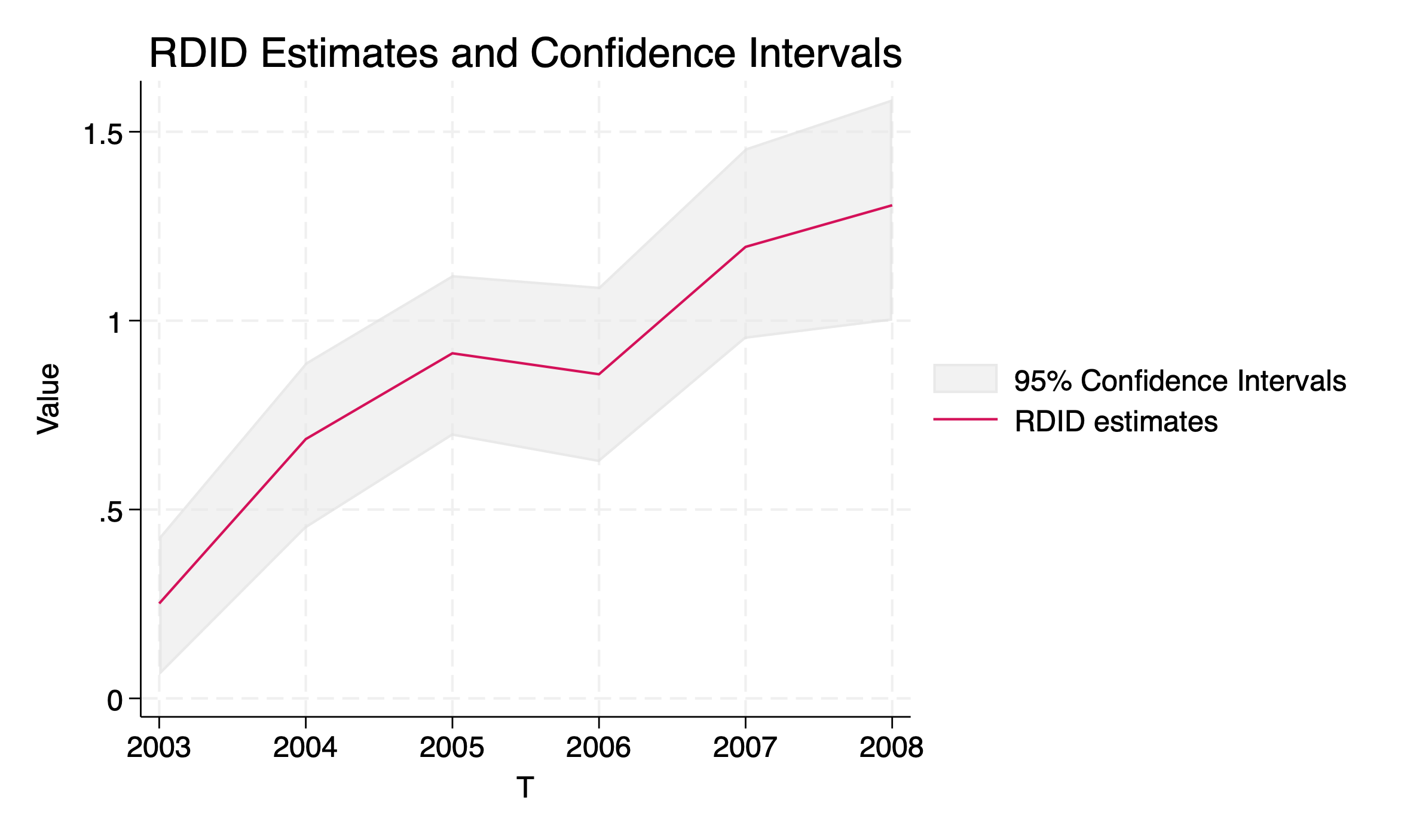
Note that rdid_dy command can be used for the option rdidtype(1) or rdidtype(2), and the following code runs for collecting PO-RDID with $\mathcal{L}_{1}$ (default), producing Figure 2 that summarizes the output.

. rdid_dy area_tob hhsize educ_scale age, rdidtype(1) treat(treatment) ///
>         post(policy2) info(year) tname(year) fig b(1000) cl(hhno)
file rdid_dy.png saved as PNG format

                                                 
        T: year      RDID_PE     CI_LB     CI_UB
                                                 
           2003       0.2513    0.0605    0.4273
           2004       0.6865    0.4497    0.8893
           2005       0.9136    0.6951    1.1206
           2006       0.8581    0.6253    1.0898
           2007       1.1953    0.9517    1.4561
           2008       1.3056    0.9999    1.5860
                                                 
* RDID estimates are obtained as PO-RDID estimates (L1)

Refer to caption — Figure 1: Figure produced by rdid_dy with rdidtype(0)

6.2 Effects of minimum wage increases on teen employment

Following Callaway and Sant’Anna (2021) and Dube et al. (2016), we used the Quarterly Workforce Indicators (QWI) data to collect the first quarter teen employment as our outcome variable. Callaway and Sant’Anna (2021) considered 7 years of periods between 2001 and 2007 where the federal minimum wage did not change over time, and 3 different control groups of $g=2004,2006,$ and $2007$ with states that raised their minimum wage in or right before the beginning of years 2004, 2006, and 2007, respectively. The specific timing of the raise can be found in Callaway and Sant’Anna (2021), and it should be noted that there is some heterogeneity in the size of the minimum wage increase within each group. The control group consists of states that did not raise their minimum wage during this period.

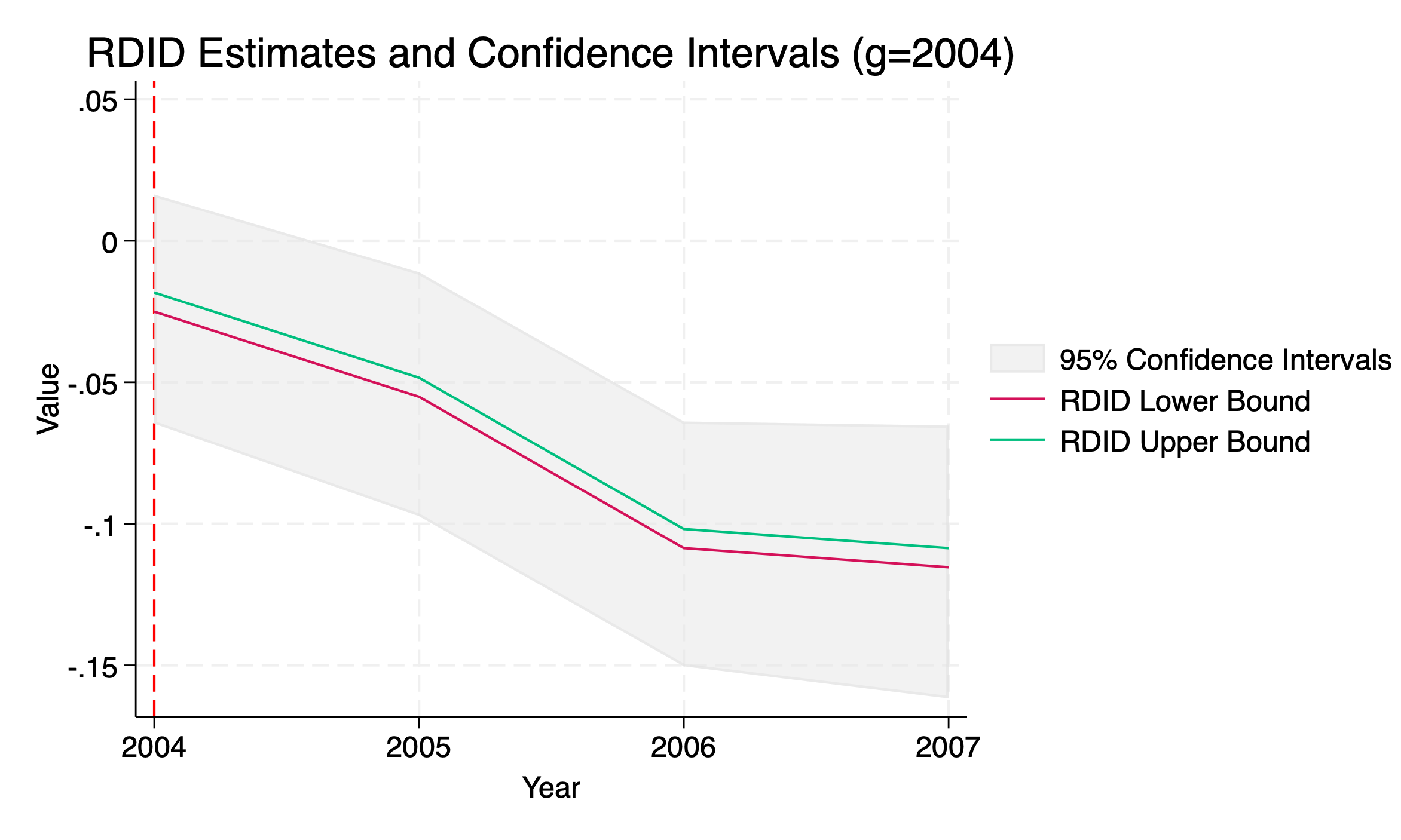
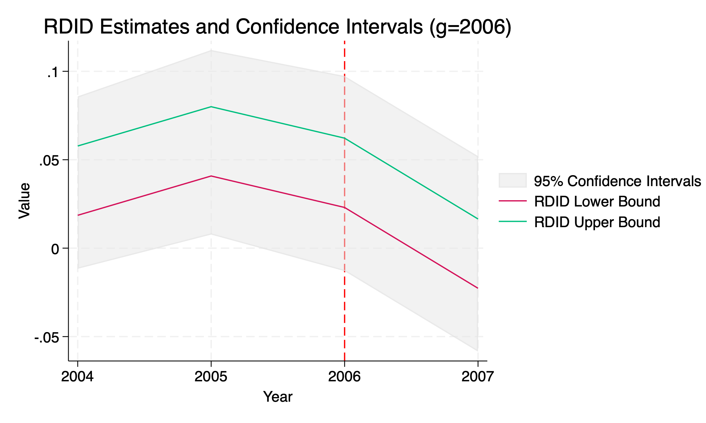
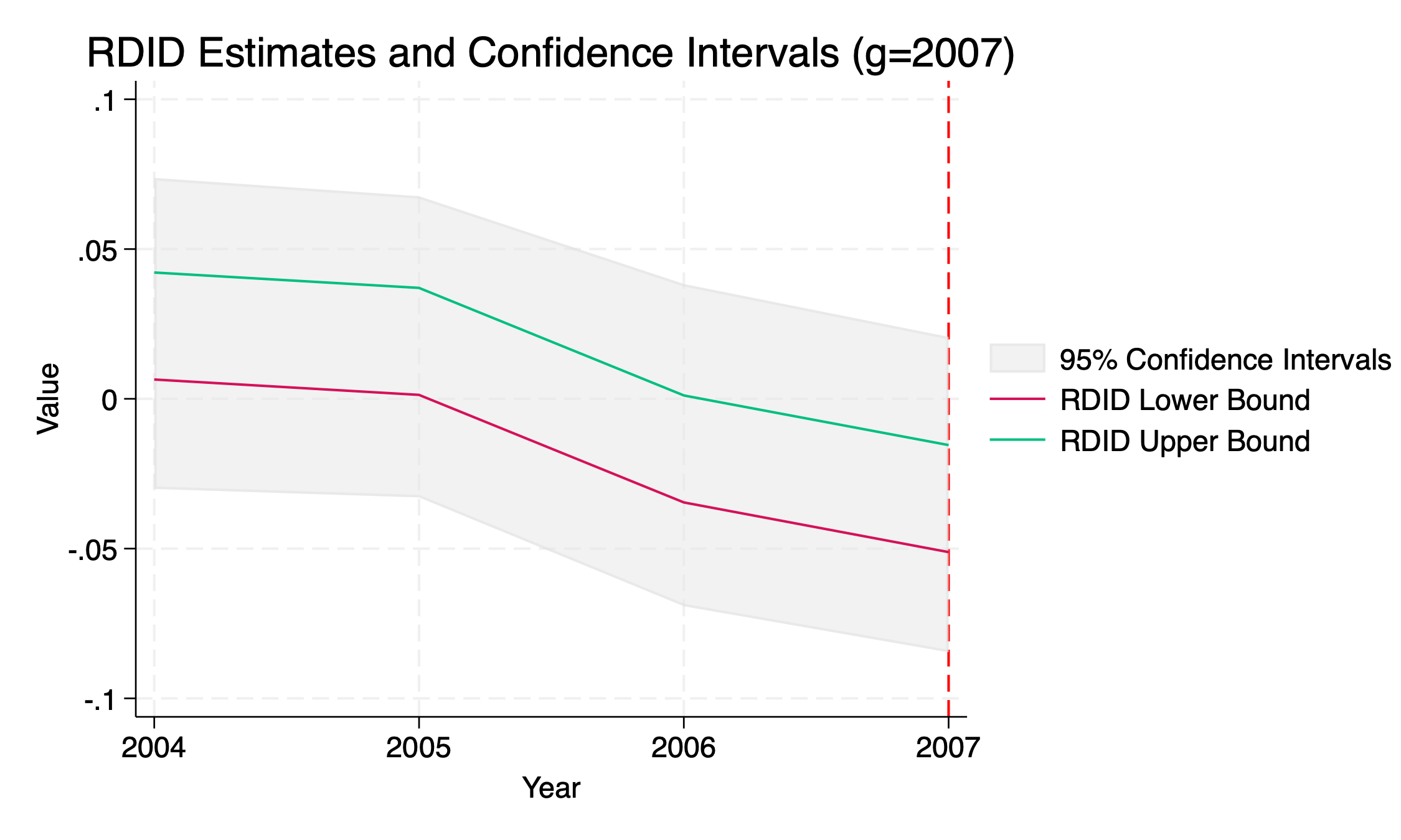
The following code specifies the option gname(G) for the cohort index variable, which has four levels: 0, 2004, 2006, and 2007. Note that because the options postname(varname) and infoname(varname) are not specified, all periods from 2004 onward are treated as post-treatment periods, and all periods before 2004 are treated as informational elements.

. use "qwi_minwageclean2.dta"

. destring years, replace
years: all characters numeric; replaced as int

. rdidstag lnemp_0A01_BS lnpop lnteenpop lnemp_0A00_BS, gname(G) tname(years) cl(countyfips) fig
 **** RDID Estimation version 1.7 ****
Y name: lnemp_0A01_BS
G name: G
X name(s): lnpop lnteenpop lnemp_0A00_BS
postname is not specified: using units with T >= min(G) as post-period units.
infoname is not specified: using pre-period T < min(G) as the information set.

                                                           
       ATT(G/T)      RDID_LB   RDID_UB   95CI_LB   95CI_UB
                                                           
 ATT(2004/2004)      -0.0250   -0.0183   -0.0646    0.0164
 ATT(2004/2005)      -0.0551   -0.0484   -0.0973   -0.0111
 ATT(2004/2006)      -0.1086   -0.1018   -0.1504   -0.0639
 ATT(2004/2007)      -0.1153   -0.1086   -0.1617   -0.0653
 ATT(2006/2004)       0.0186    0.0578   -0.0117    0.0858
 ATT(2006/2005)       0.0408    0.0800    0.0077    0.1121
 ATT(2006/2006)       0.0230    0.0622   -0.0130    0.0974
 ATT(2006/2007)      -0.0227    0.0165   -0.0585    0.0520
 ATT(2007/2004)       0.0065    0.0422   -0.0301    0.0738
 ATT(2007/2005)       0.0013    0.0370   -0.0329    0.0676
 ATT(2007/2006)      -0.0346    0.0012   -0.0692    0.0383
 ATT(2007/2007)      -0.0512   -0.0154   -0.0846    0.0207
                                                           
- Information elements: 2001 2002 2003
- Post-periods: 2004 2005 2006 2007
- Groups: 2004 2006 2007
file rdidstag_g2004.png saved as PNG format
file rdidstag_g2006.png saved as PNG format
file rdidstag_g2007.png saved as PNG format

7 Monte-Carlo Simulations

7.1 Modified Example 2: Ashenfelter’s (1978) dip

Consider

\displaystyle\left\{\begin{array}[]{lcl}Y_{it}&=&(1+|t|+t^{2})U_{i}+\theta D_{i}*t\mathbbm{1}\{t\geq 0\}+4\cdot\varepsilon_{it}\\ D_{i}&=&\mathbbm{1}\{U_{i}\geq 1\}\\ U_{i}&\sim&N(0,1)\\ \varepsilon_{it}&\sim&N(0,1)\end{array}\right.

for $t\in\mathcal{T}_{0}\cup\{1\}$ where $\mathcal{I}_{0}=\mathcal{T}_{0}=\{-2,-1,0\}$ .

In this model, $SB_{t}=(1+|t|+t^{2})(\alpha_{1}-\alpha_{0})$ where $\alpha_{1}=\frac{\phi(1)}{1-\Phi(1)}\approx 1.53$ and $\alpha_{0}=-\frac{\phi(1)}{\Phi(1)}\approx-0.29$ . We have $SB_{0}=\alpha_{1}-\alpha_{0}\neq 3(\alpha_{1}-\alpha_{0})=SB_{-1}\neq SB_{-2}=7(\alpha_{1}-\alpha_{0})$ and $SB_{0}=\alpha_{1}-\alpha_{0}\neq 3(\alpha_{1}-\alpha_{0})=SB_{1}$ . So, the standard parallel trends assumption does not hold. However, the selection bias $SB_{1}$ in period 1 belongs to the convex hull of all selection biases in period 0, i.e., $SB_{1}\in[\min\{SB_{0},SB_{-1},SB_{-2}\},\max\{SB_{0},SB_{-1},SB_{-2}\}]=[\alpha_{1}-\alpha_{0},7(\alpha_{1}-\alpha_{0})]$ . Hence, our identifying assumption holds.

We have $\theta_{OLS}=3(\alpha_{1}-\alpha_{0})+\theta$ , and $\Theta_{I}=[\theta-4(\alpha_{1}-\alpha_{0}),\theta+2(\alpha_{1}-\alpha_{0})]$ . The true $ATT=\theta$ , and the DID estimand is $\theta_{DID}=\theta_{OLS}-SB_{0}=\theta+2(\alpha_{1}-\alpha_{0})$ . Thus, the DID estimand is upward biased and the bias is equal to $2(\alpha_{1}-\alpha_{0})$ . The bounds are generally informative about the magnitude of the average treatment effect on the treated (ATT) and can identify the sign of the ATT in some circumstances. For example, when the true ATT is equal to $-5$ or $9$ , our bounds as well as the standard DID estimand identify the correct sign. On the other hand, when the true ATT is equal to $-1$ , our bounds do not identify any sign, as they contain zero. But, the standard DID estimand identifies a wrong sign, it shows that the ATT is positive while it is actually negative.

The following table shows a series of Monte-Carlo simulations for this DGP for three different confidence intervals (CIs): (1) Ye et al.’s (2023) bootstrap CI for $\Theta_{I}$ , (2) Ye et al.’s (2023) bootstrap CI for ATT, (3) union bounds for $\Theta_{I}$ .. The number of bootstrap replicates is 300, and the number of simulations is 1,000 for each case of $N\in\{200,500,1000,5000,10000,50000\}$ .

	(1) Ye et al. for bounds		(2) Ye et al. for ATT		(3) Union bounds
	$CP_{inf}$	Avg. Length	$CP_{inf}$	Avg. Length	$CP_{inf}$	Avg. Length
$N=200$	0.9300	20.7121	0.9430	20.3115	0.9610	21.1112
$N=500$	0.9540	17.1497	0.9560	16.8730	0.9620	17.2212
$N=1,000$	0.9490	15.1823	0.9490	14.9536	0.9510	15.1933
$N=5,000$	0.9510	12.8223	0.9470	12.6881	0.9510	12.8223
$N=10,000$	0.9680	12.2608	0.9610	12.1640	0.9680	12.2608
$N=50,000$	0.9640	11.4876	0.9550	11.4448	0.9640	11.4876

7.2 Example 1 from the article: with a covariate

Consider

\displaystyle\left\{\begin{array}[]{lcl}Y_{t}&=&(1+0.5^{t}X)U+\theta XD*t\mathbbm{1}\{t\geq 0\}\\ D&=&\mathbbm{1}\{U\geq 1\}\\ U&\sim&N(0,1)\\ X&\sim&Bern(p),\end{array}\right.

where $X\rotatebox[origin={c}]{90.0}{$\models$}U$ and $\mathcal{I}_{0}=\mathcal{X}=\{0,1\}$ .

We have $SB_{0}(x)=(1+x)(\alpha_{1}-\alpha_{0})$ , and $SB_{1}(x)=(1+0.5x)(\alpha_{1}-\alpha_{0})$ where $\alpha_{1}=\frac{\phi(1)}{1-\Phi(1)}\approx 1.53$ and $\alpha_{0}=-\frac{\phi(1)}{\Phi(1)}\approx-0.29$ . We have $SB_{0}(x)\in[\alpha_{1}-\alpha_{0},2(\alpha_{1}-\alpha_{0})]$ and $SB_{1}(x)\in\left[\alpha_{1}-\alpha_{0},1.5(\alpha_{1}-\alpha_{0})\right]\subseteq[\alpha_{1}-\alpha_{0},2(\alpha_{1}-\alpha_{0})]\equiv\Delta_{SB(\mathcal{X})}$ . So, the standard parallel trends assumption does not hold as $SB_{0}(x)\neq SB_{1}(x)$ . However, the selection bias $SB_{1}(x)$ in period 1 belongs to the convex hull of all selection biases in period 0, i.e., $SB_{1}(x)\in\Delta_{SB(\mathcal{X})}$ . Hence, our identifying assumption holds. We have $\theta_{OLS}(x)=(1+0.5x)(\alpha_{1}-\alpha_{0})+\theta x$ , and our new bounds $\Theta_{I}$ are obtained as $ATT(x)\in[\theta x-(1-0.5x)(\alpha_{1}-\alpha_{0}),\theta x+0.5x(\alpha_{1}-\alpha_{0})]$ . The actual conditional ATT function is $ATT(x)=\theta x$ , but the standard conditional DID estimand is $\theta_{DID}(x)=\theta x-0.5x(\alpha_{1}-\alpha_{0})$ .

Moreover, using the distribution of $X$ , we have an identified set for ATT

\Theta_{I}=\left[\left(\frac{1}{2}p-1\right)(\alpha_{1}-\alpha_{0})+p\theta,\frac{1}{2}(\alpha_{1}-\alpha_{0})+p\theta\right]

where $ATT=p\theta$ . The simulation is implemented using $p=0.5$ , and the results are presented in the following table.

	(1) Ye et al. for bounds		(2) Ye et al. for ATT		(3) Union bounds
	$CP_{inf}$	Avg. Length	$CP_{inf}$	Avg. Length	$CP_{inf}$	Avg. Length
$N=200$	0.9340	5.4190	0.9620	5.3556	0.9340	5.4190
$N=500$	0.9550	4.0948	0.9710	4.0366	0.9550	4.0948
$N=1,000$	0.9480	3.4183	0.9620	3.3703	0.9480	3.4183
$N=5,000$	0.9500	2.5282	0.9560	2.4942	0.9500	2.5282
$N=10,000$	0.9520	2.3183	0.9600	2.2887	0.9520	2.3183
$N=50,000$	0.9610	2.0405	0.9530	2.0237	0.9610	2.0405

7.3 The modified staggered adoption design

Consider

	$\displaystyle Y_{it}$	$\displaystyle=$	$\displaystyle(1+t^{2})U_{i}+\varepsilon_{it}+\sum_{s=1}^{T}\theta_{is}D_{is}\mathbbm{1}\{s\leq t\}\quad\mathrm{for}\,\,t=0,\ldots,T$
	$\displaystyle D_{it}$	$\displaystyle=$	$\displaystyle\mathbbm{1}\bigg{\{}U_{i}\geq 2-\frac{t}{T}\bigg{\}}$

where $U_{i}\rotatebox[origin={c}]{90.0}{$\models$}(\{\varepsilon_{it},\theta_{it}\}_{t=1}^{T})$ , $\theta_{it}\sim\mathcal{N}(\frac{1+t^{2}}{2},1)$ , $\mathcal{I}_{0}=\mathcal{T}_{0}=\{-T,\ldots,0\}$ , $\varepsilon_{it}\sim\mathcal{N}(t^{2},1)$ , $U_{i}\sim\mathcal{U}_{[0,2]}$ , and $T=4$ .

Note that the PT is violated as

	$\displaystyle\mathbbm{E}[Y_{it}(g^{\prime})-Y_{i0}(g^{\prime})\mid G_{i}=g]-\mathbbm{E}[Y_{it}(g^{\prime})-Y_{i0}(g^{\prime})\mid G_{i}=g^{\prime}]$
	$\displaystyle\qquad=\mathbbm{E}[t^{2}U_{i}\mid G_{i}=g]-\mathbbm{E}[t^{2}U_{i}\mid G_{i}=g^{\prime}],$
	$\displaystyle\qquad\neq 0,$

for $t>0$ when $g\neq g^{\prime}$ , especially with $g^{\prime}=\infty$ for the never-treated cohorts being the control units.

However, note that

	$\displaystyle SB_{t}[g^{\prime}\rightarrow g]$	$\displaystyle=\mathbbm{E}[Y_{it}(g^{\prime})\mid G_{i}=g]-\mathbbm{E}[Y_{it}(g^{\prime})\mid G_{i}=g^{\prime}]$
		$\displaystyle=\mathbbm{E}[(1+t^{2})U_{i}\mid G_{i}=g]-\mathbbm{E}[(1+t^{2})U_{i}\mid G_{i}=g^{\prime}],$

and

	$\displaystyle SB_{t}[g^{\prime}\rightarrow g]$	$\displaystyle\in\Delta_{SB(\mathcal{T}_{0})}[g^{\prime}\rightarrow g]$
		$\displaystyle=\bigg{[}\mathbbm{E}[U_{i}\mid G_{i}=g]-\mathbbm{E}[U_{i}\mid G_{i}=g^{\prime}],(1+T^{2})\big{(}\mathbbm{E}[U_{i}\mid G_{i}=g]-\mathbbm{E}[U_{i}\mid G_{i}=g^{\prime}]\big{)}\bigg{]},$

for all $t=1,\ldots,T$ .

In the case of $g^{\prime}=\infty$ , we have

	$\displaystyle ATT(g,t)$	$\displaystyle=\mathbbm{E}[Y_{it}(g)-Y_{it}(\infty)\mid G_{i}=g]$
		$\displaystyle=\mathbbm{E}\bigg{[}\sum_{s=g}^{T}\theta_{s}\mathbbm{1}\{s\leq t\}\bigg{]},$

and

	$\displaystyle\theta_{DIM}^{t}[\infty\rightarrow g]$	$\displaystyle=\mathbbm{E}[Y_{it}\mid G_{i}=g]-\mathbbm{E}[Y_{it}\mid G_{i}=\infty]$
		$\displaystyle=ATT(g,t)+SB_{t}[\infty\rightarrow g].$

Hence, we have

\displaystyle\Theta(g,t)

\displaystyle=\bigg{[}ATT(g,t)+(t^{2}-T^{2})\mu(g),ATT(g,t)+t^{2}\mu(g)\bigg{]},

where $\mu(g)\equiv\mathbbm{E}[U_{i}\mid G_{i}=g]-\mathbbm{E}[U_{i}\mid G_{i}=\infty]$ .

Under this setup, we implemented a series of Monte-Carlo simulations with various $N$ values, and the following tables summarize the coverage probability ( $CP_{inf}$ ) and the average length of the 95% confidence interval for each case.

Table 2: Results with

g=1

	(1) $ATT(g,1)$		(2) $ATT(g,2)$		(3) $ATT(g,3)$		(4) $ATT(g,4)$
$N$	$CP_{inf}$	Avg. Len.	$CP_{inf}$	Avg. Len.	$CP_{inf}$	Avg. Len.	$CP_{inf}$	Avg. Len.
$100$	0.9670	24.9483	0.9690	25.2785	0.9770	25.8242	0.9770	26.7418
$500$	0.9660	23.3114	0.9770	23.4608	0.9810	23.6989	0.9810	24.0988
$1000$	0.9630	22.9296	0.9710	23.0335	0.9840	23.2027	0.9810	23.4838
$5000$	0.9720	22.4170	0.9810	22.4637	0.9840	22.5398	0.9880	22.6645
$10000$	0.9680	22.2932	0.9710	22.3263	0.9820	22.3799	0.9860	22.4681

Table 3: Results with

g=2

	(1) $ATT(g,1)$		(2) $ATT(g,2)$		(3) $ATT(g,3)$		(4) $ATT(g,4)$
$N$	$CP_{inf}$	Avg. Len.	$CP_{inf}$	Avg. Len.	$CP_{inf}$	Avg. Len.	$CP_{inf}$	Avg. Len.
$100$	0.9560	20.7114	0.9660	21.0820	0.9700	21.6513	0.9700	22.5811
$500$	0.9580	19.1992	0.9720	19.3615	0.9710	19.6176	0.9740	20.0279
$1000$	0.9620	18.8385	0.9700	18.9532	0.9690	19.1349	0.9850	19.4250
$5000$	0.9610	18.3819	0.9750	18.4335	0.9830	18.5146	0.9800	18.6438
$10000$	0.9700	18.2707	0.9720	18.3071	0.9880	18.3645	0.9830	18.4559

Table 4: Results with

g=3

	(1) $ATT(g,1)$		(2) $ATT(g,2)$		(3) $ATT(g,3)$		(4) $ATT(g,4)$
$N$	$CP_{inf}$	Avg. Len.	$CP_{inf}$	Avg. Len.	$CP_{inf}$	Avg. Len.	$CP_{inf}$	Avg. Len.
$100$	0.9670	16.6965	0.9760	16.8386	0.9680	17.4816	0.9860	18.4511
$500$	0.9620	15.2021	0.9780	15.2637	0.9800	15.5432	0.9800	15.9710
$1000$	0.9580	14.8394	0.9740	14.8832	0.9880	15.0802	0.9830	15.3824
$5000$	0.9630	14.3781	0.9760	14.3974	0.9790	14.4852	0.9800	14.6201
$10000$	0.9680	14.2669	0.9730	14.2806	0.9760	14.3425	0.9770	14.4382

Table 5: Results with

g=4

	(1) $ATT(g,1)$		(2) $ATT(g,2)$		(3) $ATT(g,3)$		(4) $ATT(g,4)$
$N$	$CP_{inf}$	Avg. Len.	$CP_{inf}$	Avg. Len.	$CP_{inf}$	Avg. Len.	$CP_{inf}$	Avg. Len.
$100$	0.9690	12.7222	0.9820	12.8685	0.9820	13.3045	0.9830	14.3359
$500$	0.9590	11.2131	0.9740	11.2757	0.9820	11.4668	0.9800	11.9167
$1000$	0.9650	10.8464	0.9710	10.8904	0.9790	11.0256	0.9780	11.3440
$5000$	0.9620	10.3813	0.9740	10.4005	0.9780	10.4611	0.9760	10.6031
$10000$	0.9640	10.2689	0.9660	10.2825	0.9800	10.3252	0.9770	10.4256

8 Conclusion

In this article, we introduce the rdid, rdid_dy, and rdidstag commands to implement the RDID framework by Ban and Kédagni (2023) for both the canonical $2\times 2$ DID settings and staggered adoption designs. By allowing users to specify their information set as pre-treatment periods, the commands enhance robustness to potential violations of the parallel trends assumption in both settings. We anticipate that continued enhancements and community feedback will further increase its effectiveness and adoption in empirical research.

9 Programs and supplemental material

To obtain the latest stable versions of rdid, rdid_dy, and rdidstag from our website, refer to the installation instructions at https://github.com/KyunghoonBan/rdid.

References

Ashenfelter (1978) Ashenfelter, O. 1978. Estimating the Effect of Training Programs on Earnings. The Review of Economics and Statistics 60(1): 47–57.
Ban and Kédagni (2023) Ban, K., and D. Kédagni. 2023. Robust Difference-in-differences Models. URL https://arxiv.org/abs/2211.06710.
Bravo et al. (2022) Bravo, M. C., J. Roth, and A. Rambachan. 2022. Honestdid: Stata module implementing the honestdid r package .
Cai (2016) Cai, J. 2016. The Impact of Insurance Provision on Household Production and Financial Decisions. American Economic Journal: Economic Policy 8(2): 44–88.
Callaway and Sant’Anna (2021) Callaway, B., and P. H. Sant’Anna. 2021. Difference-in-Differences with multiple time periods. Journal of Econometrics 225(2): 200–230.
de Chaisemartin et al. (2019) de Chaisemartin, C., X. D’haultfœuille, and Y. Guyonvarch. 2019. Fuzzy differences-in-differences with stata. The Stata Journal 19(2): 435–458.
Dube et al. (2016) Dube, A., T. W. Lester, and M. Reich. 2016. Minimum Wage Shocks, Employment Flows, and Labor Market Frictions. Journal of Labor Economics 34(3): 663–704.
Han (2021) Han, S. 2021. Identification in nonparametric models for dynamic treatment effects. Journal of Econometrics 225: 132–147.
Houngbedji (2016) Houngbedji, K. 2016. Abadie’s semiparametric difference-in-differences estimator. The Stata Journal 16(2): 482–490.
Mora and Reggio (2015) Mora, R., and I. Reggio. 2015. didq: A command for treatment-effect estimation under alternative assumptions. The Stata Journal 15(3): 796–808.
Rios-Avila et al. (2023) Rios-Avila, F., P. Sant’Anna, and B. Callaway. 2023. CSDID: Stata module for the estimation of Difference-in-Difference models with multiple time periods .
Rios-Avila et al. (2022) Rios-Avila, F., P. Sant’Anna, and A. Naqvi. 2022. DRDID: Stata module for the estimation of doubly robust difference-in-difference models .
Robins (1986) Robins, J. M. 1986. A new approach to causal inference in mortality studies with a sustained exposure period–application to control of the healthy worker survivor effect. Math. Modelling 7: 1393–1512.
Robins (1987) . 1987. Addendum to “A new approach to causal inference in mortality studies with a sustained exposure period — application to control of the healthy worker survivor effect”. Comput. Math. Appl. 14(9–12): 923–945.
Villa (2016) Villa, J. M. 2016. diff: Simplifying the estimation of difference-in-differences treatment effects. The Stata Journal 16(1): 52–71.
Ye et al. (2023) Ye, T., L. Keele, R. Hasegawa, and D. S. Small. 2023. A Negative Correlation Strategy for Bracketing in Difference-in-Differences. Journal of the American Statistical Association ahead-of-print(ahead-of-print): 1–13.

rdid and rdidstag: Stata commands for robust difference-in-differences

Abstract

keywords:

1 Introduction

2 Framework and methodology

Definition 1

2.1 Bias set stability

Assumption 1 (Bias set stability)

Proposition 1

2.2 PO-RDID: Best predictor of S​B1SB_{1} based on a loss function

Assumption 2

L​1L1 loss: Mean absolute error (MAE)

L​2L2 loss: Root mean square error (RMSE)

L​∞L\infty loss: Maximal regret

2.3 Forecasting S​B1SB_{1} when the baseline information is ordered

2.4 Identification with multiple periods

Assumption 3 (Extended bias set stability)

Proposition 2

3 The rdid command

3.1 Syntax

3.2 Options

3.3 Stored results

4 The rdid_dy command

4.1 Syntax

4.2 Options

4.3 Stored results

5 The rdidstag command

5.1 Syntax

5.2 Options

5.3 Stored results

6 Applications

6.1 Effects of insurance provision on tobacco production

Using rdid command

Using rdid_dy command

6.2 Effects of minimum wage increases on teen employment

7 Monte-Carlo Simulations

7.1 Modified Example 2: Ashenfelter’s (1978) dip

7.2 Example 1 from the article: with a covariate

7.3 The modified staggered adoption design

8 Conclusion

9 Programs and supplemental material

References

2.2 PO-RDID: Best predictor of $SB_{1}$ based on a loss function

$L1$ loss: Mean absolute error (MAE)

$L2$ loss: Root mean square error (RMSE)

$L\infty$ loss: Maximal regret

2.3 Forecasting $SB_{1}$ when the baseline information is ordered