Realization of a Bosonic Antiferromagnet
Quantum antiferromagnets are of broad interest in condensed matter physics as they provide a platform for studying exotic many-body states Auerbach:2012 including spin liquids Savary:2016 and high-temperature superconductors Lee:2006 . Here, we report on the creation of a one-dimensional Heisenberg antiferromagnet with ultracold bosons. In a two-component Bose-Hubbard system, we switch the sign of the spin-exchange interaction and realize the isotropic antiferromagnetic Heisenberg model in an extended 70-site chain. Starting from a low-entropy Néel-ordered state, we use optimized adiabatic passage to approach the bosonic antiferromagnet. We demonstrate the establishment of antiferromagnetism by probing the evolution of the staggered magnetization and spin correlations of the system. Compared with condensed matter systems, ultracold gases in optical lattices can be microscopically engineered and measured, offering significant advantages for exploring bosonic magnetism and spin dynamics Gross:2017 .
For the origin of quantum magnetism in cold-atom simulator Gross:2017 , the fundamental symmetry of the constituent particles supports the general form of the spin-exchange interactions, ferromagnetic for bosons and antiferromagnetic for fermions Duan:2003 . Interestingly, the sign of the exchange interactions Trotzky:2008 and the motional degrees of freedom of atoms can be engineered by precisely controlling a staggered lattice potential, resulting in an antiferromagnetic spin model for bosons. In recent years, antiferromagnetic spin correlations have been experimentally observed in the fermionic quantum gases Greif:2013 ; Murmann:2015 ; Hart:2015 ; Boll:2016 ; Cheuk:2016 ; Mazurenko:2017 ; Drewes:2017 . However, the bosonic antiferromagnet has not been realized. Compared with fermionic atoms, besides the advantage of readily achieved lower entropy in bosonic quantum gases Yang:2020 , the tunable intra- or inter-spins interactions lead to rich phase diagrams Duan:2003 ; Altman:2003 . Additionally, unlike in Fermi-Hubbard systems where the sign problem prevents their numerical solutions, our bosonic models can enable benchmarks of numerical methods at the current state of quantum simulation in noisy intermediate-scale devices Hauke:2012 . Making use of a defect-free Mott insulator Yang:2020 , one promising approach to achieve the many-body state is via the adiabatic transformation Sorensen:2010 ; Chiu:2018 . Experimental challenges lie in engineering the Hamiltonian of two-component bosons in a many-body system and maintaining adiabaticity during the state preparation.
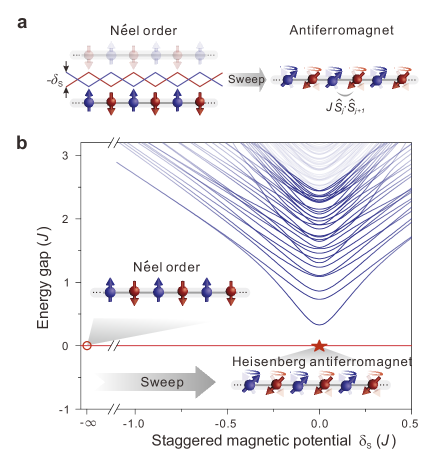
Here, we adiabatically prepare the one-dimensional (1D) antiferromagnet following the lowest-energy passage of a Heisenberg spin Hamiltonian. The experiment begins with a two-dimensional (2D) Mott insulator of 87Rb in the hyperfine state with an average filling factor of 0.992(1), which is realized based on a recently developed cooling method Yang:2020 . The hyperfine states and are defined as pseudo-spin components and , respectively. We create a spin chain in Néel order by alternatively addressing these pseudo-spin states. On this basis, Figure 1 shows that the target state can be approached by sweeping an effective staggered field Yang:2017a . We benchmark the implementation of an isotropic Heisenberg spin model by measuring its spin-relaxation dynamics. The antiferromagnet is prepared by slowly turning on the spin interactions and gradually reducing the staggering amplitude until the staggered magnetization () vanishes. We characterize the antiferromagnet by measuring local spin correlations and global spin fluctuations, reflecting a short-range antiferromagnetism in this 1D spin chain. Furthermore, we investigate its spin-rotational symmetry and robustness against dissipation.
The two-component bosons in our state-dependent optical superlattice can be well described by the Bose-Hubbard Hamiltonian,
| (1) | ||||
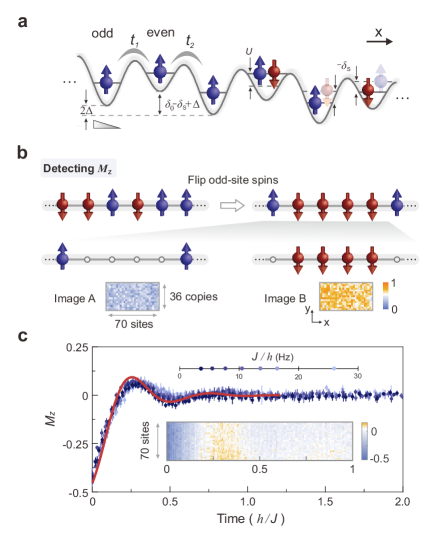
Here, the spins are indexed by ; () is the annihilation (creation) operator of an atom on site , and . In superlattice, () corresponds to the tunneling strengths on odd-even (even-odd) links; represents the on-site interaction, whose spin-dependent effect is insignificant. Figure 2a illustrates the staggered energy biases between adjacent sites, including a spin-independent term and a spin-dependent term . Additionally, a weak linear potential is applied to the 1D chain, with .
In a normal optical lattice, where and , the general Hubbard model can be mapped onto a Heisenberg-type spin model Duan:2003 . The antiferromagnetic interaction (coupling strength ) is assigned for fermions, while bosons have the ferromagnetic coupling . However, in the staggered spin-independent potential, the superexchange couplings for bosons become Trotzky:2008 . To this end, we set to reverse the sign of the superexchange coupling for both types of links, realizing the antiferromagnetic interaction with bosons throughout the chain. Meanwhile, this staggered potential localizes static motional impurities (sites filled by 0 or 2 atoms) and turns the bosonic model Lee:2006 into a spin model. Besides, we control the linear potential to unify the inter-well superexchange couplings for those two links.
Therefore, in the regime of , our system is described by the antiferromagnetic Heisenberg model after applying the Schrieffer-Wolff transformation Auerbach:2012 .
| (2) |
where are spin- operators, and represents the superexchange coupling strength by neglecting the difference between and . The staggered magnetic field originates from the spin-dependent term in the Hamiltonian (1). For characterizing this -site antiferromagtism, the staggered magnetization is introduced as, .
When , the ground state of is a Néel-ordered state as , see Fig. 1. In this spin-balanced system, the lowest-energy excitation corresponds to flipping an arbitrary spin pair, like . The opposite Néel order state, , represents the ground state at . The ground state at is our target antiferromagnet . This is a highly-entangled many-body state, exhibiting zero but strong spin correlations. Due to the SU(2) symmetry of , this ground state naturally gains the spin-rotational invariance. The ground and the first-excited states are separated by a minimal energy gap of . The state can be approached by slowly sweeping the from to 0, while the small energy gap and the intrinsic heating Ho:2007 ; Yang:2020 impose limitations on the adiabaticity.
In the experiment, atoms are confined by a superlattice potential along the -axis, as . Here, the wavelengths of short- and long-lattice lasers are 767 nm and 1534 nm; are lattice depths and represents their relative phase. A deep short-lattice along the -axis isolates the system into copies of 1D chains. To initialize the Néel order, a spin-dependent superlattice is applied to split the degeneracy of the hyperfine-transition frequencies between odd and even sites Yang:2017a . Then all the atoms resided on odd sites are flipped to . Here, a region of interest (ROI) containing sites is selected for analysis. Consequently, 36 copies of 70-site 1D chains are prepared in the Néel order with an entropy per particle of ( is the Boltzmann constant), acting as the ground state of the spin model at .
We engineer the spin-dependent superlattice potential to implement the many-body spin model. To enable the inter-well coupling Trotzky:2008 ; Greif:2013 ; Yang:2020 , the most pronouncing staggered potential emerges at . However, such a superlattice gives rise to insignificant spin-dependent effects. To ensure sufficient values of both and , we set the phase to and turn on the spin-dependent effect. For compensating the discrepancy between the superexchange couplings in two types of links, we employ the gravity to project a linear potential on the 1D chain. Furthermore, the Hubbard parameters , and are mainly controlled by tuning the depths of lattices.
We investigate the spin relaxations by quenching the system to activate the Heisenberg model at . The is measured by utilizing the same sub-wavelength addressing technique, whereafter the atomic densities of the spin components are recorded on two images A and B, see Figure 2b. Thereby, the local averaged staggered magnetization is expressed as, . Figure 2c shows the spin dynamics with ranging from 3.6(1) Hz to 26.0(5) Hz, which collapse into a single curve when the evolution time is rescaled by . Rather than a barely incoherent decay, a coherent oscillatory spin evolution is clearly observed in this many-body system. We perform the time-adaptive density matrix renormalization group (-DMRG) method to calculate the dynamics of this 70-site spin chain. Our results agree excellently with the theoretical predictions, indicating a faithful realization of the many-body antiferromagnetic model.
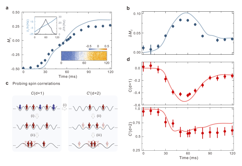
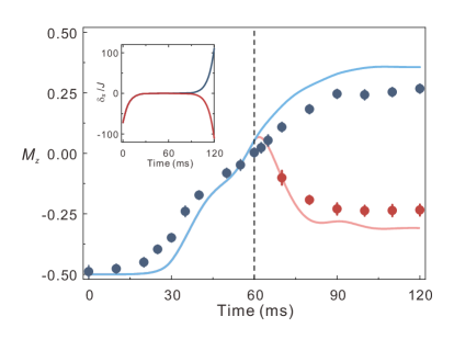
We realize the antiferromagnet by ramping and simultaneously, whose ratio determines the adiabaticity. One notable property of the antiferromagnet is the vanished . However, a high-entropy state which remarkably populates the high-energy excited levels could also manifest . To optimize the adiabatic passage, we continue the ramping and reach a large positive . From the revival of , we could infer the entropy of the target system, which simply increases as more high-energy levels are populated. Figure 3a shows the optimized ramping process, which begins with and the system finally achieves a low-entropy antiferromagnet within 60 ms.
We observe an enhancement of spin fluctuations during the establishment of the antiferromagnetic state. The fluctuations of can be formulated as . We extract by subtracting the detection noise and spatial broadening effects from the measurements (see methods). Figure 3b shows that grows up gradually during the 60 ms sweep. The fluctuation decays as the ramp process continues towards the positive .
The state is quantified by measuring its nearest- and next-nearest-neighbor spin correlations. The correlation function is expressed as, , where is the distance between lattice sites. Here, we probe the spin correlations by first manipulating the atomic states in the superlattice, and then detecting double occupations with a photoassociation process Yang:2020 . The procedure for extracting is sketched as (i)-(ii) in Figure 3c. (i) The spin component is removed from the lattice confinement. (ii) We combine the atoms on the neighboring sites with the superlattice. The doublons are then removed by a photoassociation laser. Therefore, the probability of the spin states equals to the atom-loss in this stage. The other spin states can be detected by rotating them to before the step (i). Thus, . Figure 3d shows the establishment of this spin correlation, which reaches the largest value at 60 ms.
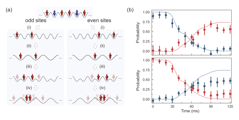
Similarly, Figure 3c shows the procedure for probing the next-nearest-neighbor correlation. In (i), we remove the atoms resided on the even sites and all the spin- atoms on the odd sites. (ii) The atoms are split in one superlattice configuration with , where they have the same probability to enter each side. (iii) We combine the atoms with the double-well superlattice at . The atom correlation is also measured by counting the photoassociation-induced particle loss. Actually, this probing method can only be used to detect the correlation between identical spins in the next-nearest-neighbor sites, defined as . Figure 3d shows during the spin dynamics, where the state probabilities are corrected by incorporating the particle-hole excitations. At 60 ms, the correlation shows that the spin orientations tend to be identical in the next-nearest-neighbor sites. Here, as the staggered magnetization vanishes, the spin correlations indicate the existence of entanglement among the spin chain.
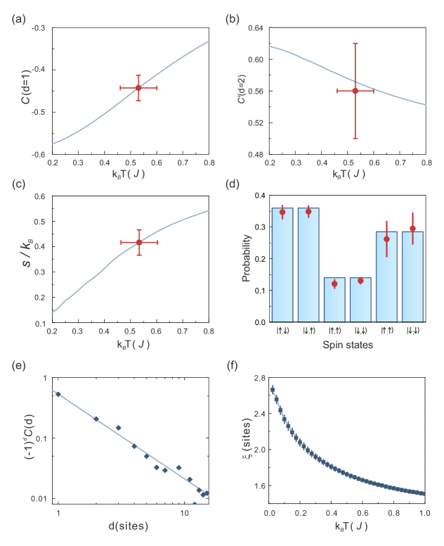
Ideally, a fully adiabatic sweep will end up with the opposite Néel order state, like . However, in Figure 3, our numerical calculations show imperfect revival of the state, which is due to the nonadiabaticity of the sweep. Besides, our experiment has some discrepancy with the numerics, which can be attributed to the motional excitations in the Bose-Hubbard chain as well as the intrinsic heating arising from the incoherent laser scattering Yang:2020 . Comparing the measured with a finite-temperature quantum Monte Carlo calculation of the spin chain, we can infer an effective entropy per particle of (see methods) and a temperature of . The temperature is still far larger than the energy gap around the critical point. However, the zero-temperature simulation is in good agreement with the experiment measurement, suggesting that such a finite temperature does not affect the adiabatic passage. Due to the enhanced quantum fluctuations in 1D systems, the correlation function follows a power-law decay behavior. Our theoretical simulation shows that the spin correlation is short-range and the correlation length does not diverge even when the temperature approaches zero (see method).
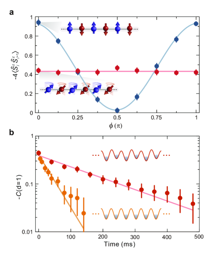
As the antiferromagnet is generated at 60 ms of the adiabatic passage, we observe its spin rotational symmetry by measuring the spin correlation after global spin rotations. When a Rabi pulse is applied on this state, all spins are rotated around -axis by an angle . Subsequently, the spin correlation is extracted. Figure 4a shows that this correlation function maintains constant for the antiferromagnet. For comparison, the initial Néel-ordered state is also measured following the same procedure. In the absence of entanglement between atoms, it behaves like a single spin under rotations. The spin-rotational invariance of our state is consistent with the SU(2) symmetry of the Hamiltonian.
The robustness of the antiferromagnet is measured by holding the atoms in the strong-coupling regime, where Hz and . Figure 4b shows the slow decay of , whose lifetime 183(13) ms is 4.8(4) times of the exchange period . The staggered potential freezes the motions of the particles, and thus the decay is mainly caused by spin excitations Dimitrova:2020 . This further explains the strong correlations of the state prepared through the adiabatic sweeping. For comparison, we also monitor the damping of the correlation under the ferromagnetic spin-exchange coupling in the single-frequency lattice. As shown in Figure 4b, the nearest-neighbor correlation decays much faster and the lifetime 39(4) ms equals to 1.1(1) and 3.0(3). In the absence of staggered potential as , the dynamics of the system is governed by the bosonic model Lee:2006 , where the free propagation of the particle-hole excitations makes the antiferromagnet melt rapidly. Therefore, our staggered potential represents a powerful tool for preserving the spin correlations, which could be used for protecting the spin states in other types of Hubbard systems or the highest-energy state of spin models Sorensen:2010 . In a doped antiferromagnet, by controlling this staggered potential, we can transform the Heisenberg spin model to a model and activate the interplay between spin and motional degrees of freedom for investigating the out-of-equilibrium spin dynamics.
In summary, we have demonstrated the creation of a Heisenberg antiferromagnet with ultracold bosons in optical lattices. Our adiabatic passage circumvents the difficulties of directly cooling the atoms in the gapless phases. In the near future, interesting topics include studying the competition between spin and charge excitations during the build-up of the antiferromagnet Hilker:2017 ; Chiu:2019 , cooling the spin degrees of freedom Yang:2020 and detecting the thermalization of the antiferromagnetic spin chain Pozsgay:2014 . Based on the low entropy achieved in such a large system, we can further investigate the transport properties of the spin or charge excitations in the long-wavelength limit Haldane:1981 ; Giamarchi:2004 ; Nichols:2019 ; Brown:2019 ; Vijayan:2020 ; Jepsen:2020 . Besides, the multipartite entanglement in the antiferromagnet could be certified aiming for applications in quantum metrology Almeida:2020 . Furthermore, by subtly controlling the spin gaps White:1994 and tailoring our uniform system with a recently developed addressing technique Yang:2020s , our method could be extended to higher-dimensional systems, to explore the resonating valence-bond states Nascimbene:2012 and also topological phases stabilized by the multi-body interactions Dai:2017 .
Acknowledgements.
Acknowledgement We thank Philipp Hauke, Eugene Demler and Gang Chen for helpful discussions. This work is supported by National Key R&D Program of China grant 2016YFA0301603, NNSFC grant 11874341, the Fundamental Research Funds for the Central Universities, the Anhui Initiative in Quantum Information Technologies, and the Chinese Academy of Sciences.Author contributions B.Y., Z.-S.Y. and J.-W.P. conceived and designed this research. B.Y, H.-N.D., Z.-S.Y. and J.-W.P built the experimental apparatus. H.S, B.Y, H.-Y.W., Z.-Y.Z. and G.-X.S. performed the experiments and analysed the data. All authors contributed to manuscript preparation.
Data availability Data for figures that support the current study are available at https://doi.org/10.7910/DVN/GPMPMP
Code availability Numerical simulations were performed with python code that makes use of the OpenMPS Library available at https://openmps.sourceforge.io/ and the ALPS project available at http://alps.comp-phys.org/. Python source codes are available from the corresponding authors on request.
Competing interests The authors declare no competing interests.
References
- (1) Auerbach, A. Interacting Electrons and Quantum Magnetism (Springer-Verlag, 2012).
- (2) Savary, L. & Balents, L. Quantum spin liquids: a review. Rep. Prog. Phys. 80, 016502 (2016).
- (3) Lee, P. A., Nagaosa, N. & Wen, X.-G. Doping a Mott insulator: Physics of high-temperature superconductivity. Rev. Mod. Phys. 78, 17–85 (2006).
- (4) Gross, C. & Bloch, I. Quantum simulations with ultracold atoms in optical lattices. Science 357, 995–1001 (2017).
- (5) Duan, L.-M., Demler, E. & Lukin, M. D. Controlling spin exchange interactions of ultracold atoms in optical lattices. Phys. Rev. Lett. 91, 090402 (2003).
- (6) Trotzky, S. et al. Time-resolved observation and control of superexchange interactions with ultracold atoms in optical lattices. Science 319, 295–299 (2008).
- (7) Greif, D., Uehlinger, T., Jotzu, G., Tarruell, L. & Esslinger, T. Short-range quantum magnetism of ultracold fermions in an optical lattice. Science 340, 1307–1310 (2013).
- (8) Murmann, S. et al. Antiferromagnetic Heisenberg spin chain of a few cold atoms in a one-dimensional trap. Phys. Rev. Lett. 115, 215301 (2015).
- (9) Hart, R. A. et al. Observation of antiferromagnetic correlations in the Hubbard model with ultracold atoms. Nature 519, 211–214 (2015).
- (10) Boll, M. et al. Spin- and density-resolved microscopy of antiferromagnetic correlations in Fermi-Hubbard chains. Science 353, 1257–1260 (2016).
- (11) Cheuk, L. W. et al. Observation of spatial charge and spin correlations in the 2D Fermi-Hubbard model. Science 353, 1260–1264 (2016).
- (12) Mazurenko, A. et al. A cold-atom Fermi-Hubbard antiferromagnet. Nature 545, 462–466 (2017).
- (13) Drewes, J. H. et al. Antiferromagnetic correlations in two-dimensional fermionic Mott-insulating and metallic phases. Phys. Rev. Lett. 118, 170401 (2017).
- (14) Yang, B. et al. Cooling and entangling ultracold atoms in optical lattices. Science 369, 550–553 (2020).
- (15) Altman, E., Hofstetter, W., Demler, E. & Lukin, M. D. Phase diagram of two-component bosons on an optical lattice. New J. Phys. 5, 113–113 (2003).
- (16) Hauke, P., Cucchietti, F. M., Tagliacozzo, L., Deutsch, I. & Lewenstein, M. Can one trust quantum simulators? Rep. Prog. Phys. 75, 082401 (2012).
- (17) Sørensen, A. S. et al. Adiabatic preparation of many-body states in optical lattices. Phys. Rev. A 81, 061603(R) (2010).
- (18) Chiu, C. S., Ji, G., Mazurenko, A., Greif, D. & Greiner, M. Quantum state engineering of a Hubbard system with ultracold Fermions. Phys. Rev. Lett. 120, 243201 (2018).
- (19) Yang, B. et al. Spin-dependent optical superlattice. Phys. Rev. A 96, 011602(R) (2017).
- (20) Ho, T.-L. & Zhou, Q. Intrinsic heating and cooling in adiabatic processes for bosons in optical lattices. Phys. Rev. Lett. 99, 120404 (2007).
- (21) Dimitrova, I. et al. Enhanced superexchange in a tilted Mott insulator. Phys. Rev. Lett. 124, 043204 (2020).
- (22) Hilker, T. A. et al. Revealing hidden antiferromagnetic correlations in doped Hubbard chains via string correlators. Science 357, 484–487 (2017).
- (23) Chiu, C. S. et al. String patterns in the doped Hubbardmodel. Science 365, 251–256 (2019).
- (24) Pozsgay, B. et al. Correlations after Quantum Quenches in the XXZ Spin Chain: Failure of the Generalized Gibbs Ensemble. Phys. Rev. Lett. 113, 117203 (2014).
- (25) Haldane, F. D. M. Luttinger liquid theory of one-dimensional quantum fluids. I. Properties of the Luttinger model and their extension to the general 1D interacting spinless Fermi gas. J. Phys. C: Solid State Phys. 14, 2585–2609 (1981).
- (26) Giamarchi, T. Quantum physics in one dimension (Oxford University Press, Oxford, 2004).
- (27) Nichols, M. A. et al. Spin transport in a Mott insulator of ultracold fermions. Science 363, 383–387 (2019).
- (28) Brown, P. T. et al. Bad metallic transport in a cold atom Fermi-Hubbard system. Science 363, 379–382 (2019).
- (29) Vijayan, J. et al. Time-resolved observation of spin-charge deconfinement in fermionic Hubbard chains. Science 367, 186–189 (2020).
- (30) Jepsen, N. et al. Spin transport in a tunable Heisenberg model realized with ultracold atoms. Nature 588, 403–407 (2020).
- (31) de Almeida, R. C. & Hauke, P. From entanglement certification with quench dynamics to multipartite entanglement of interacting fermions. ArXiv https://arxiv.org/abs/2005.03049 (2020).
- (32) White, S. R., Noack, R. M. & Scalapino, D. J. Resonating Valence Bond Theory of Coupled Heisenberg Chains. Phys. Rev. Lett. 73, 886–889 (1994).
- (33) Yang, B. et al. Observation of gauge invariance in a 71-site Bose-Hubbard quantum simulator. Nature 587, 392–396 (2020).
- (34) Nascimbène, S. et al. Experimental realization of plaquette resonating valence-bond states with ultracold atoms in optical superlattices. Phys. Rev. Lett. 108, 205301 (2012).
- (35) Dai, H.-N. et al. Four-body ring-exchange interactions and anyonic statistics within a minimal toric-code Hamiltonian. Nat. Phys. 13, 1195–1200 (2017).
METHODS AND SUPPLEMENTARY MATERIALS
.1 Experimental system
Our experiment begins with a nearly pure Bose-Einstein condensate of 87Rb prepared in the hyperfine state of . Then, we increase the confinement along the axis and load the atoms into a single node of a 3- spacing blue-detuned lattice to create a quasi-2D quantum gas. The confinement in the plane is provided by a red-detuned optical dipole trap propagating along the direction. To prepare a low-entropy Mott insulator, we implement a newly-developed cooling technique in optical lattices. In the cooling process, the entropy of the Mott insulator is transferred into the contacting superfluid reservoirs. In our region of interest (36 copies of 70-site chains), the probability of unity-filling for the Mott insulator is 0.992(1).
To initialize the Néel order along the -direction, we employ a site-selective spin addressing technique to overcome the optical diffraction limit. The atomic Mott insulator is transferred into an spin-dependent superlattice Yang:2017a which breaks the odd-even symmetry of the lattice sites and thereby separates the atoms into two subsystems. For odd and even subsystems, the lattice potentials are controlled to split their transition frequencies between and hyperfine levels. By applying an edited microwave pulse, we flip the atoms of odd sites into with an efficiency of 0.995(3) through a rapid adiabatic passage. For each site, the preparation fidelity of the Néel state can be estimated as 0.987(3). Therefore, in the 70-site chain, a defect-free Néel order is achieved with a probability of 40%.
.2 Staggered potentials
The superlattice naturally forms staggered potentials for our ground-band ultracold atoms. Here, we make use of two distinct effects of the superlattice, which are the spin-dependent and the spin-independent effects. Such an optical potential can be expressed as,
| (S1) |
where is the wave vector of the short-lattice laser; is the spin-dependent phase shift of the short-lattice, and denotes the two spin states. The original trap depth of short-lattice is also altered to two spin-dependent terms , and . At , the superlattice is simplified to the spin-independent form, . By tuning the applying voltage of an electro-optical modulator, we can control the spin-dependent energy with a bandwidth larger than 20 kHz Yang:2017a .
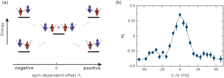
The spin-dependent energy shift can be precisely controlled in our system. To calibrate the zero-energy point , we perform a spectroscopy measurement of spin-exchange dynamics in isolated double-wells. We prepare the atoms in state and then quench the superlattice to , and . Here, is the recoil energy with the Planck constant and the atomic mass. In this balanced structure, the resonating superexchange frequency within double wells is Hz. The inter-well coupling is forbidden by the long-lattice barrier. The degeneracy of the states and is lifted by a nonzero spin-dependent effect. As we scan the and monitor the staggered magnetization , a clear spectroscopy of the spin exchange dynamics is observed, as shown in Extended Data Fig. 1. The position of the central peak can be determined with a precision of 0.4 Hz. In addition, the energy offsets of the side peaks agree well with our calculations based on the lattice structure.
.3 Establishing the isotropic Heisenberg Hamiltonian
We design a special 1D superlattice along the -direction for realizing the isotropic antiferromagnetic Heisenberg model. When , the inter-well coupling becomes comparably strong as the intra-well coupling. In this 1D chain, there are two types of links connecting the neighboring sites, which can be denoted as odd-even (type I) and even-odd (type II) links. At , these two types of links are identical to each other, while the spin-dependent effect will disappear in this configuration. To enable the spin-dependent term, we set the superlattice phase to and keep the long-lattice depth at . The tunneling strength on the type II links is roughly 10 percent larger than on the type I links Walters:2013s .
In the second-order perturbation theory, the spin exchange coupling along these two types of links are,
| (S2) |
Here, and represent energy offsets between neighboring sites due to the spin-independent term and a linear potential, respectively. and are tunneling strengths along the two types of nearest-neighbor links. Since the lattice depths are almost the same for the two spin states, the tunneling strengths are independent of spin components. corresponds to the on-site interaction for all the spin states. Here we neglect the slight spin-dependence of scattering lengths for 87Rb and adopt . When , we reverse the sign of and to positive, establishing an antiferromagnetic spin-exchange coupling Trotzky:2008 .
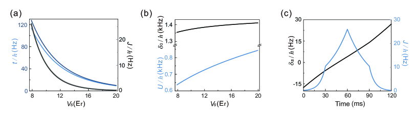
The difference between the spin exchange couplings and is compensated by the state-independent linear potential. Since our -axis lies at an angle of 4 degree related to the horizontal plane, the gravity leads to a constant 57-Hz/site gradient along the 1D chain. Consequently, the discrepancy between and is less than 2 percent [see Extended Data Fig. 2(c)], one order of magnitude lower than the case without this compensation ( and would have 20 percent difference in the absence of such a linear potential).
Under our experimental conditions, the Hubbard parameters satisfy such relations , as shown in Extended Data Fig. 2. We should stress that even though atoms tend to occupy the low-energy sites owing to the non-uniform potential along the 1D chain, the atoms cannot overcome the staggered potential via tunneling in our experimental relevant time scale. Therefore, the Bose-Hubbard Hamiltonian can be mapped into a spin model as,
| (S3) |
By neglecting the slight difference between and , we can adopt the geometric mean of them as , and write the Hamiltonian as an isotropic Heisenberg model.
We can understand the spin model in two extreme cases. In the limit of , the two types of Néel orders are the ground states of the system. In another limit, , unlike the Ising-type spin model, this Heisenberg model has a single energetic ground state . The SU(2) symmetry of this isotropic Hamiltonian leads to the same rotational symmetry of this ground state.
.4 Adiabatic passage
Starting from the initial Néel-ordered state , we experimentally optimize the ramping curves to minimize the non-adiabaticity to approach the Heisenberg antiferromagnet . The lattice with 42.0(3) isolates the system into 36 copies of 70-site 1D chains. The superlattice phases are switched to before ramping down the short-lattice potential.
Then, we slowly ramp the lattice potentials in terms of the Hubbard parameters. At 0 ms, the staggered magnetic gradient is Hz, and the coupling strength is Hz. During the 60 ms ramping, we separate the curve into two stages with 30-ms intervals, as shown in Extended Data Fig. 2(c). The coupling strength and the staggered gradient are increased gradually during the sweep. At 60 ms, is slightly larger than 0, but the zero value of the staggered magnetization indicates the achievement of a Heisenberg antiferromagnet. In another 60 ms, we ramp back the lattice potentials slowly and increase oppositely. The system is driven towards the opposite Néel order with , implying the low-entropy property of the antiferromagnet. To detect the property of the state at each time, we freeze the state by quenching the lattice barrier to disable the atom dynamics.
Starting from the prepared antiferromagnet, we apply another adiabatic protocol to the system by ramping reversely after 60 ms to a large negative value (see Extended Data Fig. 3). Finally, can return to , which means the decoherence and nonadiabaticity of the system can be well distinguished.
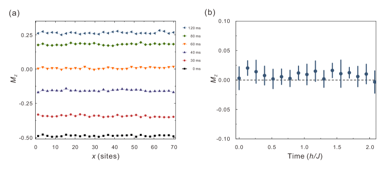
We quantify the translational symmetry of the antiferromagnet. Extended Data Fig. 4(a) shows that the measured does not gain any spatial periodicity. Such phenomena is consistent with the translational-invariant property of the antiferromagnet. Besides, we hold the atoms in the strong coupling regime after the 60-ms adiabatic passage, where Hz and . As shown in Extended Data Fig. 4(b), maintains almost constant and does not exhibit any oscillations, which suggests that the created state is close to thermal equilibrium.
.5 Nearest-neighbor spin correlation
The atomic densities are detected via an absorption imaging with 1 m spatial resolution. Even though the imaging process is destructive, we can record the density distributions of both spin states () in two successive images. We choose a region of interest (ROI) containing 36 copies of 70-site 1D chains in the center of the atomic cloud for the statistical analysis.
The nearest-neighbor correlation function is defined as,
| (S4) |
where represents the number of sites. In our spin-balanced system, the second term in the sum is equal to the square of the staggered magnetization, as . The first term in the sum is obtained by averaging the correlated measurements on two types of links, as . The correlation functions are given as following,
| (S5) |
Here, represent the probabilities of spin states on the corresponding links. Making use of the superlattice, we can combine the atoms on neighboring sites into a single lattice well. These two types of links are measured at two kinds of superlattice configurations, one has and the other has . Depending on the atom number on the combined site, we can derive the desired probabilities.
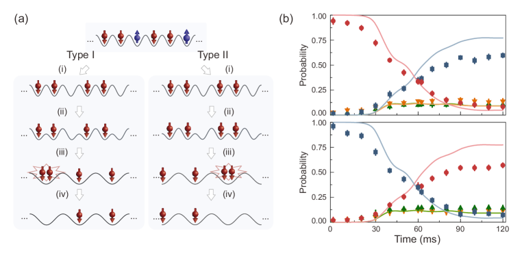
We probe the parity of site occupations by applying a photoassociation (PA) laser to the atomic sample. The laser is red-detuned to the D2 line of 87Rb by 13.6 , which has an intensity of 0.56 and lasts for 20 ms. Assisted by this laser, atom pairs in hyperfine state can be excited to the vibrational state of the long-range molecular channel Fioretti:2001s . This unstable molecule would decay back to free atoms and gain kinetic energy to escape from the trap. Therefore, the ratio of atom loss is equivalent to the probability of the state before the combining operation. The detection scheme is illustrated in Extended Data Fig. 5(a), where two sets of measurements are carried out for these two types of links. In this way, we obtain the probabilities of , as shown in Extended Data Fig. 5(b).
For the other spin states , we employ the site-selective spin addressing technique to transfer them into the state before implementing the detection procedures Yang:2017a . For instance, we flip all of the atoms on odd sites for probing the probabilities and . Finally, the probabilities of these four states allow us to calculate the spin correlation . However, all of the measurement errors would propagate into the final results. We use the basic normalization condition to reduce the errors by only taking the residual atoms in the last step of Extended Data Fig. 5(a) into calculations.
In Extended Data Fig. 5(b), the probabilities of the four spin state for type I and type II nearest-neighbor links are depicted. The deviation from the numerical calculations is mainly caused by the motional excitations in Hubbard model and the lattice heating during the adiabatic passage. Besides, the inefficiency of the state manipulations accumulates and finally reduces the detected spin correlations.
.6 Motional excitations
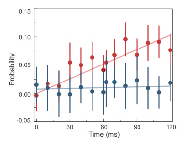
Besides spin excitations, the particle-hole excitations emerge when the atoms tunnel to their neighboring sites. Such motional excitations are detected by counting the ratio of doublons making use of the parity-projection technique. Using a global spin-flip, we can acquire the doublons on the state as well. However, atoms have to tunnel to their next-nearest-neighbor sites in order to create such identical-spin doublons. Extended Data Fig. 6 shows that the excitations to the state and are generally rare [1(1) percent] in the adiabatic passage.
The more probable motional excitations are original from the atoms that tunnel to their neighboring sites and therefore result in the doublons. From the normalization condition, the ratio of these excitations can be deduced as , with . As shown in Extended Data Fig. 6, the ratio of this type of motional excitations grows gradually during the state evolution, which is 0.04(3) for our target state. The propagation of such excitations is strongly suppressed by the spin-independent staggered offset . Besides, the linear potential also suppresses the long-range motional transport Yang:2020s .
.7 Next-nearest-neighboring spin correlation
According to the Mermin-Wagner-Hohenberg theorem Mermin:1966s , the 1D isotropic Heisenberg Hamiltonian cannot support a long-range spin order Yang:2017s . As the distance grows, the magnetic correlation decays rapidly in the 1D Heisenberg antiferromagnetic state. So the occurrence of nonzero next-nearest-neighbor spin correlation would be a distinctive signature of approaching a low-entropy antiferromagnet.
However, without a site-resolved imaging, the superlattice structure normally only provides the access to the nearest-neighbor spin correlation because of its translational symmetry Trotzky:2010s ; Dai:2016s . Here, owing to our precise control of the superlattice phase, we can extend the capability of the correlated spin measurement to next-nearest-neighbor links.
Extended Data Figure 7(a) shows the procedure of detecting the probability of spin state in next-nearest-neighboring links. After a selective atom removal, the superlattice serves as an array of atomic splitters to redistribute the remaining atoms into their adjacent sites with equal probabilities. Subsequently, changing the superlattice phase by , we can transfer the atoms originally lying two sites apart to the same long-lattice unit in a probabilistic way. The atom loss in a PA collision can be used to deduce the probability of spin state . Similarly, the state on next-nearest-neighbor sites can be detected with an additional global spin-flip pulse before the step (i).
We define a next-nearest-neighbor correlator as,
| (S6) |
where and represent the probabilities of spin state and on next-nearest-neighbor links. These probabilities equal to four times of the corresponding atom losses in the PA collision. For determining the probabilities accurately, we subtract the contribution of the motional excitations in the PA collision.
Extended Data Figure 7(b) shows the variations of the probabilities and for odd- and even-sites respectively. Since only a quarter of atoms contribute to the signal, the probabilities measured here have larger errors compared to their counterparts on nearest-neighbor links.
.8 Numerical simulation
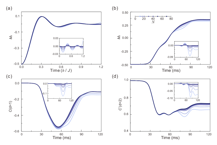
Based on the Heisenberg spin model, the numerical results for both the post-quench dynamics and the adiabatic passage are calculated using the -DMRG algorithm in the framework of matrix product states. In the numerics, we neglect the slight difference between the spin-exchange couplings of the two types of links and adopt their geometric mean in the spin model. We implement the methods using the OpenMPS library Jaschke:2018s and fix the maximal bond dimension to . Convergence are achieved at a time step of and s for the quench dynamics and the adiabatic passage, respectively. The truncation threshold is per time step. We investigate the finite-size effects by calculating the spin dynamics in 1D systems at several sizes . As shown in Extended Data Fig. 8, the discrepancy between the curves for and is on the order of , indicating the volume convergence of our calculations.
Temperature and entropy of the state are estimated by comparing the experimental results with finite-temperature quantum Monte Carlo methods (QMC) Bauer:2011s . All the simulations are carried out in the grand-canonical ensemble on a 70-site open chain. In such a large system, the finite-size effect can be eliminated. After times of thermalization, we continue to perform the QMC sweeps for at least times to get the results under each setting. We choose the temperature from 0.2 to 0.8 with a 0.03 interval.
From the nearest-neighbor correlation of interest [], we derive the temperature of our system to be 0.53(7), see Extended Data Fig. 9(a). In Extended Data Fig. 9(b), we present the next-nearest-neighbor correlation as a function of the temperature. At a temperature of 0.53(7), reaches 0.57(1) in this thermal state. The entropy per particle is obtained using another QMC method, which is called quantum Wang-Landau algorithm Wang:2001s . The cutoff of series expansion is set to be . As shown in Extended Data Fig. 9(c), the entropy per particle deduced from the temperature of the spin chain is 0.42(5).
Based on the comparison between the measured probabilities of the spin state and the prediction of the thermalized state, our system is inferred to be a thermalized state, see Extended Data Fig. 9(d).
From the -DMRG simulations, we plot the spin correlations of the antiferromagnet up to 15 sites. As shown in Extended Data Fig. 9(e), the correlation function exhibits a power-law decay as the distance increases, which is consistent with the property of the Tomanaga-Luttinger Liquid Haldane:1981 ; Giamarchi:2004 ; Yang:2017s .
.9 Fluctuations of the staggered magnetization
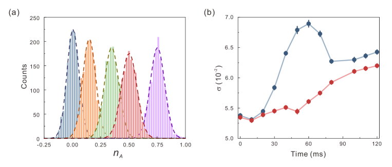
The spin fluctuations in terms of can reflect non-local spin correlations of many-body states. However, the detection of is obstructed by the detection noise, for instance the shot noise of our absorption imaging. Here, we develop a method to resolve the spin fluctuations on the basis of the two-image measurements. The total density corresponds to a unit-filling Mott insulator with vanishing density fluctuations. Since the staggered magnetization is , where the spin fluctuations only exist on . In this respect, we can extract directly from the fluctuations of . For reference, we consider the background fluctuations due to the photon shot-noise by analyzing the total density . We resolve the spin fluctuations by subtracting the shot-noise background, as .
As Extended Data Fig. 10 (a) shows, the density histogram of throughout the adiabatic sweep are obtained by counting the densities on 2.37 copies 70-site chains (one pixel equals to 2.37 sites). Based on 100 experimental repetitions, we acquire 1500 groups of measurement for each histogram. Here, represents the Gaussian waist of the histogram of (the Gaussian function is used for fitting), as shown in Extended Data Fig. 10 (b). Taking into account the imaging resolution and the pixel size, the fluctuation of staggered magnetization can be extracted.
References
- (1) Walters, R., Cotugno, G., Johnson, T. H., Clark, S. R. & Jaksch, D. Ab initio derivation of Hubbard models for cold atoms in optical lattices. Phys. Rev. A 87, 043613 (2013).
- (2) Fioretti, A. et al. Cold rubidium molecule formation through photoassociation: A spectroscopic study of the long-range state of 87Rb2. Eur. Phys. J. D 15, 189–198 (2001).
- (3) Mermin, N. D. & Wagner, H. Absence of ferromagnetism or antiferromagnetism in one- or two-dimensional isotropic Heisenberg models. Phys. Rev. Lett. 17, 1133–1136 (1966).
- (4) Yang, B. et al. Quantum criticality and the Tomonaga-Luttinger liquid in one-dimensional bose gases. Phys. Rev. Lett. 119, 165701 (2017).
- (5) Trotzky, S., Chen, Y.-A., Schnorrberger, U., Cheinet, P. & Bloch, I. Controlling and detecting spin correlations of ultracold atoms in optical lattices. Phys. Rev. Lett. 105, 265303 (2010).
- (6) Dai, H.-N. et al. Generation and detection of atomic spin entanglement in optical lattices. Nat. Phys. 12, 783–787 (2016).
- (7) Jaschke, D., Wall, M. L. & Carr, L. D. Open source matrix product states: Opening ways to simulate entangled many-body quantum systems in one dimension. Comput. Phys. Commun. 225, 59 – 91 (2018).
- (8) Bauer, B. et al. The ALPS project release 2.0: open source software for strongly correlated systems. J. Stat. Mech. Theor. Exp. 2011, P05001 (2011).
- (9) Wang, F. & Landau, D. P. Efficient, multiple-range random walk algorithm to calculate the density of states. Phys. Rev. Lett. 86, 2050–2053 (2001).