Realm: Real-Time Line-of-Sight Maintenance in Multi-Robot Navigation with Unknown Obstacles

Existing works considering connectivity maintenance can be categorized into continuous and discrete types [9]. Continuous connectivity requires robots to always maintain a connected network during their operations. Giordano et al. propose a potential function-based method that guarantees connectivity by preserving the Fiedler eigenvalue of the underlying graph Laplacian to be positive [11, 9]. In their work, the LoS constraints are captured by the distance from the closest obstacle point to the LoS segment joining two robots. Alternatively, an analytical form of the LoS constraints is also derived in [14] by approximating the LoS segment with a minimum volume enclosing ellipsoid (MVEE). Chen et al. also consider the LoS constraints in multi-UAV deployment [13], where the movements of two robots are restricted in a safe zone defined by separating hyperplanes of obstacles.

In contrast, discrete connectivity only requires robots to be connected at certain time steps [15]. A typical procedure first determines a target connected topology for the robots based on spanning tree search, after which their positions are refined through local optimization to balance additional objectives such as travel distance or information gain [4, 16, 17, 10]. To ensure LoS constraints in the local optimization stage, Stump et al. apply polygonal decomposition of an environment, after which neighboring robots’ positions are restricted in a common polyhedron to ensure LoS [16]. Xia et al. formulate the LoS constraints based on robots’ visible regions described by star convex polytope [10]. However, as local optimization modifies robots’ positions, the corresponding changes in their visible regions may lead to potential LoS loss after optimization.

While most existing works rely on known environment models described by either obstacle points [11, 14] or occupancy maps [16, 10], few works have considered connectivity maintenance in unknown environments. Li et al. propose a reinforcement learning-based approach that generates control commands based on the inputs of range sensor measurements and the positions of other robots, and does not rely on prior environmental information [18]. However, the method has no guarantee of global connectivity.

Given a graph $\mathcal{G}=\langle\mathcal{V},\mathcal{E}\rangle$ with $N$ vertices, the graph Laplacian matrix of $\mathcal{G}$ is defined as $\mathbf{L}=D-A$, where $A\in\mathbb{R}^{N\times N}$ is the adjacency matrix with an element $A_{ij}=0$ if $(i,j)\notin\mathcal{E}$, and $A_{ij}>0$ otherwise; $D\in\mathbb{R}^{N\times N}$ is a diagonal degree matrix where $D_{ii}=\sum_{j=1}^{N}A_{ij}$ and $D_{ij}=0$ when $i\neq j$. The second-smallest eigenvalue $\lambda_{2}$ of $\mathbf{L}$, usually referred to as the Fiedler eigenvalue [19] or connectivity eigenvalue, can be used to check the connectivity of the graph $\mathcal{G}$. It holds the property that $\lambda_{2}>0$ if the graph $\mathcal{G}$ is connected, or $\lambda_{2}=0$ otherwise.

By encoding the satisfaction levels of different kinds of connectivity constraints between two robots into the weight of their corresponding edge, the Fiedler eigenvalue $\lambda_{2}$ of the weighted graph Laplacian can be used to reflect the generalized graph connectivity [11]. In this work, we also use this concept to ensure connectivity between robots by enforcing that the Fiedler eigenvalue $\lambda_{2}$ of the weighted graph Laplacian remains positive during navigation.

As shown in Fig. 2(a), given the point cloud measurement $\mathcal{C}_{j}\subseteq\mathbb{R}^{3}$ from the robot $j$, its visible region can be constructed via the following steps [20, 21, 10]:

1) Augmentation. Add augmented points to fill the gaps in the point cloud $\mathcal{C}_{j}$;

2) Spherical flipping. Map each point $\mathbf{\boldsymbol{q}}\in\mathcal{C}_{j}$ along the ray originating from the robot $j$ to a point $\mathbf{\boldsymbol{q}}^{\prime}$ located outside a sphere of radius $r$, following the equation $\mathbf{\boldsymbol{q}}^{\prime}=2r\cdot\frac{\mathbf{\boldsymbol{q}}}{\|\mathbf{\boldsymbol{q}}\|}-\mathbf{\boldsymbol{q}}$. The flipped point cloud is denoted as $\mathcal{C}_{j}^{\prime}$;

3) Convex hull construction. Generate convex hull of $\mathcal{C}_{j}^{\prime}$, denoted as $Conv(\mathcal{C}_{j}^{\prime})$.

4) Inversion. Inverse the convex hull by performing the inverse spherical flipping. The inversed shape of the convex hull encloses the visible region of robot $j$.

As shown in Fig. 2(a), the visibility of a point $\mathbf{\boldsymbol{q}}_{i}\in\mathbb{R}^{3}$ from the position $\mathbf{\boldsymbol{q}}_{j}\in\mathbb{R}^{3}$ of robot $j$ is determined by the distance $d_{k^{*}}$, defined as $d_{k^{*}}=\max_{k}\{d_{k}=\mathbf{\boldsymbol{n}}_{k}^{\top}(\mathbf{\boldsymbol{q}}_{i}^{\prime}-\boldsymbol{a}_{k})|k=1,...,K\}$, where $\mathbf{\boldsymbol{n}}_{k}$ is the outward normal vector of the $k$-th face of $Conv(\mathcal{C}_{j}^{\prime})$ composed of $K$ faces; $\boldsymbol{a}_{k}\in\mathbb{R}^{3}$ is an arbitrary point on the face $k$; $\mathbf{\boldsymbol{q}}_{i}^{\prime}$ is the flipped point of $\mathbf{\boldsymbol{q}}_{i}$ following the spherical flipping; and the index $k^{*}$ is defined as $k^{*}=\arg\max_{k\in[1,...,K]}d_{k}$. If $d_{k^{*}}>0$, $\mathbf{\boldsymbol{q}}_{i}$ is visible from $\mathbf{\boldsymbol{q}}_{j}$, i.e., they are within line-of-sight with each other; vice verse if $d_{k^{*}}\leq 0$. The log-sum-exp relaxation is employed to get a differentiable approximation of $d_{k^{*}}$, defined as

$$d_{k^{*}}\approx\frac{1}{\alpha}\log\left(e^{\alpha d_{1}}+\cdots+e^{\alpha d_{K}}\right),$$

(1)

where $\alpha>0$ is a coefficient that controls the degree of approximation [21]. The above process is adopted from the hidden point removal (HPR) operator in point cloud visibility analysis [20], with time complexity of $\mathcal{O}(n\log n)$, where $n$ is the size of a point cloud.

In this paper, we aim to derive the LoS constraints between robots from their point cloud measurements. Specifically, we first construct the visible regions of robots, and then design potential functions to keep them operating within each other’s visible regions to maintain LoS connectivity.

Assume there are a set of robots $\mathcal{R}=\{1,2,...,R\}$ to perform navigation tasks in an initially unknown environment. The position and orientation of a robot $i\in\mathcal{R}$ at time $t$ is denoted as $\mathbf{\boldsymbol{q}}_{i}(t)\in\mathbb{R}^{3}$ and $R_{i}(t)\in\mathcal{SO}(3)$ respectively. We assume the kinematic model of robot $i$ is a single-integrator as follows:

$$\mathbf{\boldsymbol{q}}_{i}(t+1)=\mathbf{\boldsymbol{q}}_{i}(t)+k^{\text{c}}_{i}\cdot\boldsymbol{u}^{\text{c}}_{i}(t)+k^{\text{n}}_{i}\cdot\boldsymbol{u}^{\text{n}}_{i}(t),$$

(2)

where $\boldsymbol{u}^{\text{c}}_{i},\boldsymbol{u}^{\text{n}}_{i}\in\mathbb{R}^{3}$ are the velocity commands for connectivity and navigation, respectively; $k_{i}^{\text{c}},k_{i}^{\text{n}}\in\mathbb{R}_{\geq 0}$ are two scaling factors. Moreover, the combined velocity command is bounded by $\|k^{\text{c}}_{i}\cdot\boldsymbol{u}^{\text{c}}_{i}(t)+k^{\text{n}}_{i}\cdot\boldsymbol{u}^{\text{n}}_{i}(t)\|_{2}\leq U_{\text{max}}$, where $U_{\text{max}}\in\mathbb{R}_{+}$ is the upper limit of robots’ velocities.

Let $\mathcal{G}(t)=\langle\mathcal{V},\mathcal{E}(t),\omega\rangle$ be an undirected time-varying graph, where $\mathcal{V}=\{1,...,R\}$ includes $R$ vertices that correspond to robots in $\mathcal{R}$; $\mathcal{E}(t)\subseteq\mathcal{V}\times\mathcal{V}$ is the edge set at time $t$; and the weighting function $\omega:\mathcal{V}\times\mathcal{V}\xrightarrow{}\mathbb{R}_{\geq 0}$ evaluates the strength of connectivity between two vertices in the graph. The relative distance between two robots $i,j\in\mathcal{R}$ is defined as $d_{ij}=d_{ji}=\lVert\mathbf{\boldsymbol{q}}_{i}-\mathbf{\boldsymbol{q}}_{j}\rVert_{2}$. An edge $(i,j)\in\mathcal{E}$ if and only if the following conditions are satisfied:

• •

  (C1) Communication constraints. The relative distance between two robots $i$ and $j$ must be within the communication range $d^{\text{com}}$, i.e., $d_{ij}\leq d^{\text{com}}$.

• •

  (C2) Line-of-Sight constraints. The two robots must be within each other’s line-of-sight, i.e., $\eta\mathbf{\boldsymbol{q}}_{i}+(1-\eta)\mathbf{\boldsymbol{q}}_{j}\notin\mathcal{O}$, $\forall\eta\in[0,1]$, where $\mathcal{O}\subseteq\mathbb{R}^{3}$ includes obstacles in the environment that are unknown to the robots.

• •

  (C3) Collision avoidance constraints. The relative distance between robot $i$ and robot $j$, and their distance to surrounding obstacles must be larger than a safe distance $d^{\text{coll}}$, i.e., $d_{ij}\geq d^{\text{coll}}$.

We define a set $\mathcal{N}_{i}=\{j\in\mathcal{V}|(i,j)\in\mathcal{E}\}$ as the collection of all neighboring robots of robot $i$ that satisfy above constraints. The graph $\mathcal{G}$ is referred to as the connectivity graph of the robot team. Initially, we assume $\mathcal{G}(0)$ is connected.

Given a sequence of target points $\mathcal{Z}=\{\boldsymbol{z}^{1},...,\boldsymbol{z}^{M}\}\subseteq\mathbb{R}^{3}$ distributed in the free space of an unknown environment, and a group of robots $\mathcal{R}=\{1,...,R\}$ with kinematic models as in Eq. (2). We assume $M\leq R$. The index of the designated robot to a target $\boldsymbol{z}^{m}\in\mathcal{Z}$ is denoted as the robot $i_{z}^{m}$. The problem is to find a sequence of velocity commands $\boldsymbol{u}^{\text{c}}_{i}$ and $\boldsymbol{u}^{\text{n}}_{i}$ for each robot $i\in\mathcal{R}$ so that: (1) there exist a time sequence $0\leq t^{1},...,t^{M}<\infty$ when the corresponding target $\boldsymbol{z}^{m}$ is visited by the assigned robot $i_{z}^{m}$ at time $t^{m}$, and stay at $\boldsymbol{z}^{m}$ for a pre-defined time duration $\Delta T$; (2) the connectivity graph $\mathcal{G}(t)$ is connected for $\forall t\geq 0$.

The unknown obstacles present challenges for LoS maintenance between robots during navigation, which is our main focus in this paper. In contrast, the formulations of communication constraints (C1) and inter-robot collision avoidance (part of C3) only depend on robots’ relative distances, which can be derived following [11]. The details are provided in the Appendix for completeness.

Based on the concept of generalized graph connectivity, we define $\omega(i,j)=A_{ij}=\alpha_{ij}\cdot\beta_{ij}\cdot\gamma_{ij}$ for an edge $(i,j)\in\mathcal{E}$ in the connectivity graph, where $\alpha_{ij},\beta_{ij},\gamma_{ij}\in\mathbb{R}_{\geq 0}$ are the weights quantifying the satisfaction of constraints C1, C2, and C3 between two robots $i$ and $j$, respectively. We define a potential function $V^{\lambda}(\lambda_{2})=\frac{1}{\lambda_{2}-\lambda_{2}^{\text{min}}}$ to enforce the Fiedler eigenvalue $\lambda_{2}$ of $\mathcal{G}$ being larger than a preferred lower bound $\lambda_{2}^{\text{min}}>0$ as in [11, 12]. Then the velocity command for a robot $i\in\mathcal{R}$ to maintain the graph connectivity can be derived as [22]

$$\small\boldsymbol{u}^{\text{c}}_{i}=-\frac{\partial V^{\lambda}(\lambda_{2})}{\partial\lambda_{2}}\cdot\frac{\partial\lambda_{2}}{\partial\mathbf{\boldsymbol{q}}_{i}}=-\frac{\partial V^{\lambda}(\lambda_{2})}{\partial\lambda_{2}}\cdot\sum_{j\in\mathcal{N}_{i}}\frac{\partial A_{ij}}{\partial\mathbf{\boldsymbol{q}}_{i}}(v_{2_{i}}-v_{2_{j}})^{2},$$

where $v_{2_{i}}$ and $v_{2_{j}}$ are respectively the $i$-th and $j$-th elements of the normalized eigenvector $\boldsymbol{v}_{2}$ corresponding to the $\lambda_{2}$.

In subsequent sections, we will focus on the formulation of $\beta_{ij}(\cdot)$ to quantify the LoS constraints between robots, while the definitions of $\alpha_{ij}(\cdot)$ and $\gamma_{ij}(\cdot)$ are provided in the Appendix due to space limitations.

This section presents a LoS-distance metric that quantifies both the urgency and sensitivity of losing LoS between two robots. While the distance $d_{k^{*}}$ as in Eq. (1) can be used to determine the visibility between two robots, it cannot quantify the sensitivity of losing LoS as a robot moves. The situation is illustrated in Fig. 3(a), where, although the two cases have the same $d_{k^{*}}$, the change of $d_{k^{*}}$ after applying a delta movement to the test point is significantly different.

Here we quantitatively analyze the sensitivity of robot $i$ losing LoS with robot $j$, i.e., moving beyond the visible region of robot $j$. To begin with, the position of robot $i$ in robot $j$’s local coordinate frame is obtained by $\mathbf{\boldsymbol{q}}_{ji}=R_{j}^{-1}(\mathbf{\boldsymbol{q}}_{i}-\mathbf{\boldsymbol{q}}_{j})\in\mathbb{R}^{3}$. Recall in Sec. III-B, the flipped point of $\mathbf{\boldsymbol{q}}_{ji}$ is calculated as $\mathbf{\boldsymbol{q}}_{ji}^{\prime}=2r\cdot\frac{\mathbf{\boldsymbol{q}}_{ji}}{\lVert\mathbf{\boldsymbol{q}}_{ji}\rVert}-\mathbf{\boldsymbol{q}}_{ji}$. To quantify the sensitivity of losing LoS, we introduce a disturbance movement $\delta\mathbf{\boldsymbol{q}}$ to $\mathbf{\boldsymbol{q}}_{ji}$, defined as $\delta\mathbf{\boldsymbol{q}}=\xi_{1}\cdot\mathbf{\boldsymbol{e}}_{r}+\xi_{2}\cdot\mathbf{\boldsymbol{e}}_{t}+\xi_{3}\cdot\mathbf{\boldsymbol{e}}_{n}$, where $\xi_{1},\xi_{2},\xi_{3}\in\mathbb{R}$; $\|\delta\mathbf{\boldsymbol{q}}\|\leq\sigma\in\mathbb{R}_{+}$ with $\sigma\xrightarrow{}0$; $\mathbf{\boldsymbol{e}}_{r},\mathbf{\boldsymbol{e}}_{t},\mathbf{\boldsymbol{e}}_{n}$ are orthogonal basis vectors in radial, tangential, and normal directions. The notations are illustrated in Fig. 3(b) in 2D cases. Note that $\mathbf{\boldsymbol{e}}_{r}$ is parallel to $\mathbf{\boldsymbol{n}}_{r}$, defined as $\mathbf{\boldsymbol{n}}_{r}=\frac{\mathbf{\boldsymbol{q}}_{ji}^{\prime}}{\|\mathbf{\boldsymbol{q}}_{ji}^{\prime}\|}$. After applying the delta movement to $\mathbf{\boldsymbol{q}}_{ji}$, the resulting movement of $\mathbf{\boldsymbol{q}}_{ji}^{\prime}$ is $\delta\mathbf{\boldsymbol{q}}^{\prime}\approx-\xi_{1}\cdot\mathbf{\boldsymbol{e}}_{r}+\frac{2r-\|\mathbf{\boldsymbol{q}}_{ji}\|}{\|\mathbf{\boldsymbol{q}}_{ji}\|}(\xi_{2}\cdot\mathbf{\boldsymbol{e}}_{t}+\xi_{3}\cdot\mathbf{\boldsymbol{e}}_{n})$. By projecting to the normal direction $\mathbf{\boldsymbol{n}}_{k^{*}}$, the resulting change of $d_{k^{*}}$ is $\Delta_{d_{k^{*}}}=(\delta\mathbf{\boldsymbol{q}}^{\prime})^{\top}\mathbf{\boldsymbol{n}}_{k^{*}}\approx-\xi_{1}\cos{\theta_{k^{*}}}+\frac{2r-\|\mathbf{\boldsymbol{q}}_{ji}\|}{\|\mathbf{\boldsymbol{q}}_{ji}\|}(\xi_{2}+\xi_{3})\sin{\theta_{k^{*}}}$. Considering $\xi_{1},\xi_{2},\xi_{3}\xrightarrow{}0$ and that the flipping radius $r$ is typically set to be much larger than $\|\mathbf{\boldsymbol{q}}_{ji}\|$, we omit the term $-\xi_{1}\cos{\theta_{k^{*}}}$ and get

$$\small\Delta_{d_{k^{*}}}\approx\frac{2r-\|\mathbf{\boldsymbol{q}}_{ji}\|}{\|\mathbf{\boldsymbol{q}}_{ji}\|}(\xi_{2}+\xi_{3})\sin{\theta_{k^{*}}}\leq\frac{2r-\|\mathbf{\boldsymbol{q}}_{ji}\|}{\|\mathbf{\boldsymbol{q}}_{ji}\|}\cdot\sqrt{2}\sigma\cdot\sin{\theta_{k^{*}}}.$$

According to the above expression, in the worst case, the sensitivity of $d_{k^{*}}$ w.r.t. the robot’s delta movement is determined by $\sin{\theta_{k^{*}}}$, i.e., a larger $|\theta_{k^{*}}|$ will introduce larger potential decrease of $d_{k^{*}}$, and vice versa. The analysis is aligned with the illustrations in Fig. 3(a).

Therefore, we define a sensitivity-encoded LoS-distance metric that quantifies the distance from robot $i$ to the visible region of robot $j$ as $\hat{d}^{\text{los}}_{ji}=d_{k^{*}}\cdot\cos{\theta_{k^{*}}}$. A differentiable approximation of this metric is defined as

$$\small\hat{d}^{\text{los}}_{ji}=\frac{1}{\alpha}\log(\sum_{k=1}^{K}e^{\alpha d_{k}})\cdot\frac{\sum_{k=1}^{K}e^{\alpha d_{k}}\cdot\cos{\theta_{k}}}{\sum_{k=1}^{K}e^{\alpha d_{k}}},$$

(3)

where $\cos{\theta_{k}}=\mathbf{\boldsymbol{n}}_{r}^{\top}\mathbf{\boldsymbol{n}}_{k}$. The rationale behind this metric is, to increase $\hat{d}^{\text{los}}_{ji}$, the movement of robot $i$ should not only contribute to a larger $d_{k^{*}}$ (to reduce urgency), but also a larger $\cos{\theta_{k^{*}}}$ to reduce the sensitivity of losing LoS with robot $j$. The derivative of $\hat{d}^{\text{los}}_{ji}$ w.r.t. $\mathbf{\boldsymbol{q}}_{ji}^{\prime}$ is calculated as

	$\displaystyle\frac{\partial\hat{d}^{\text{los}}_{ji}}{\partial\mathbf{\boldsymbol{q}}_{ji}^{\prime}}=$	$\displaystyle\cos{\hat{\theta}_{k^{*}}}\cdot\hat{\mathbf{\boldsymbol{n}}}_{k^{*}}^{\top}+\frac{\hat{d}_{k^{*}}}{\|\mathbf{\boldsymbol{q}}_{ji}^{\prime}\|}(\hat{\mathbf{\boldsymbol{n}}}_{k^{*}}^{\top}-\cos{\hat{\theta}_{k^{*}}}\cdot\mathbf{\boldsymbol{n}}_{r}^{\top})$		(4)
		$\displaystyle+\alpha\cdot\hat{d}_{k^{*}}(\frac{\widehat{\cos{\theta_{k^{*}}}\cdot\mathbf{\boldsymbol{n}}_{k^{*}}^{\top}}}{\cos{\hat{\theta}_{k^{*}}}}-\hat{\mathbf{\boldsymbol{n}}}_{k^{*}}^{\top}),$

where $\cos{\hat{\theta}_{k^{*}}}=\frac{\sum e^{\alpha d_{k}}\cdot\cos{\theta_{k}}}{\sum e^{\alpha d_{k}}}$; $\hat{\mathbf{\boldsymbol{n}}}_{k^{*}}^{\top}=\frac{\sum e^{\alpha d_{k}}\cdot\mathbf{\boldsymbol{n}}_{k}^{\top}}{\sum e^{\alpha d_{k}}}$; $\hat{d}_{k^{*}}=\frac{\hat{d}^{\text{los}}_{ji}}{\cos{\hat{\theta}_{k^{*}}}}$; $\widehat{\cos{\theta_{k^{*}}}\cdot\mathbf{\boldsymbol{n}}_{k^{*}}^{\top}}=\frac{\sum e^{\alpha d_{k}}(\cos{\theta_{k}}\cdot\mathbf{\boldsymbol{n}}_{k}^{\top})}{\sum e^{\alpha d_{k}}}$. Assuming ideal log-sum-exp approximation, Eq. (4) can be simplified as

$$\frac{\partial\hat{d}^{\text{los}}_{ji}}{\partial\mathbf{\boldsymbol{q}}_{ji}^{\prime}}\approx\cos{\theta_{k^{*}}}\cdot\mathbf{\boldsymbol{n}}_{k^{*}}^{\top}+\frac{d_{k^{*}}}{\|\mathbf{\boldsymbol{q}}_{ji}^{\prime}\|}(\mathbf{\boldsymbol{n}}_{k^{*}}^{\top}-\cos{\theta_{k^{*}}}\cdot\mathbf{\boldsymbol{n}}_{r}^{\top}).$$

(5)

Note that when $\theta_{k^{*}}=0$, i.e., $\mathbf{\boldsymbol{n}}_{k^{*}}=\mathbf{\boldsymbol{n}}_{r}$, the derivative is calculated as $\frac{\partial\hat{d}^{\text{los}}_{ji}}{\partial\mathbf{\boldsymbol{q}}_{ji}^{\prime}}\Big{|}_{\theta_{k^{*}}=0}\approx\mathbf{\boldsymbol{n}}_{k^{*}}^{\top}$, which is the same as the derivative when using Eq. (1) to measure the LoS-distance.

Finally, the derivative of $\hat{d}^{\text{los}}_{ji}$ w.r.t. $\mathbf{\boldsymbol{q}}_{ji}$ is calculated as

$$\frac{\partial\hat{d}^{\text{los}}_{ji}}{\partial\mathbf{\boldsymbol{q}}_{ji}}=\frac{\partial\hat{d}^{\text{los}}_{ji}}{\partial\mathbf{\boldsymbol{q}}_{ji}^{\prime}}\cdot\frac{\partial\mathbf{\boldsymbol{q}}_{ji}^{\prime}}{\mathbf{\boldsymbol{q}}_{ji}}=\frac{\partial\hat{d}^{\text{los}}_{ji}}{\partial\mathbf{\boldsymbol{q}}_{ji}^{\prime}}(\frac{2r}{\|\mathbf{\boldsymbol{q}}_{ji}\|}-\frac{2r}{\|\mathbf{\boldsymbol{q}}_{ji}\|^{3}}\cdot\mathbf{\boldsymbol{q}}_{ji}\mathbf{\boldsymbol{q}}_{ji}^{\top}-1).$$

This section proposes the potential function $\beta(\cdot)$ that encodes the LoS-distances between the robots $i$ and $j$ into the weight of the edge $(i,j)\in\mathcal{E}$. To ensure that they are within each other’s LoS, it is required that $\hat{d}^{\text{los}}_{ij},\hat{d}^{\text{los}}_{ji}\geq 0$.

However, directly designing a potential function for $\hat{d}^{\text{los}}_{ij}$ and $\hat{d}^{\text{los}}_{ji}$ is not applicable, because it is often the case that $\hat{d}^{\text{los}}_{ij}\neq\hat{d}^{\text{los}}_{ji}$, which will finally lead to asymmetric values of the edge weights $A_{ij}$ and $A_{ji}$. In fact, the different values of $\hat{d}^{\text{los}}_{ij}$ and $\hat{d}^{\text{los}}_{ji}$ reflect the imbalanced urgency of losing LoS for two robots, as illustrated in Fig. 2(b). To keep the Laplacian matrix symmetric, we need to find a differentiable function to fuse $\hat{d}^{\text{los}}_{ij}$ and $\hat{d}^{\text{los}}_{ji}$ while reflecting the urgency of losing LoS between the two robots. As such urgency is determined by the smaller value between $\hat{d}^{\text{los}}_{ij}$ and $\hat{d}^{\text{los}}_{ji}$, an intuitive option is to use a differentiable approximation of the $\min(\cdot)$ function such as $\text{Softmin}(\cdot)$ function to take the smaller value. However, this will lead to poor cooperation between robots to maintain LoS, as verified in Sec. VII-B.

To address this issue, we define a LoS-distance fusion function $d^{\text{los}}(\cdot)$ as

$$\small d^{\text{los}}_{ij}=\frac{\hat{d}^{\text{los}}_{ij}+c}{\hat{d}^{\text{los}}_{ij}+\hat{d}^{\text{los}}_{ji}+2c}\cdot\hat{d}^{\text{los}}_{ji}+\frac{\hat{d}^{\text{los}}_{ji}+c}{\hat{d}^{\text{los}}_{ij}+\hat{d}^{\text{los}}_{ji}+2c}\cdot\hat{d}^{\text{los}}_{ij}$$

(6)

when $\hat{d}^{\text{los}}_{ij},\hat{d}^{\text{los}}_{ji}\geq d^{\text{los}}_{\text{min}}$. The Eq. (6) is essentially a weighted sum of $\hat{d}^{\text{los}}_{ij}$ and $\hat{d}^{\text{los}}_{ji}$, where $c\in\mathbb{R}_{\geq 0}$ is a constant parameter that controls whether $d^{\text{los}}_{ij}$ depends more on the smaller value among $\hat{d}^{\text{los}}_{ij}$ and $\hat{d}^{\text{los}}_{ji}$ (when $c$ takes a small value) or their averaged value (otherwise). Particularly, the gradient of $d^{\text{los}}_{ij}$ w.r.t. $\hat{d}^{\text{los}}_{ij}$ and $\hat{d}^{\text{los}}_{ji}$ is less imbalanced that using the $\text{Softmin}(\cdot)$ function, and can be regulated by the parameter $c$, which facilitates the less urgent robot’s movement to maintain LoS with its more urgent neighbor.

According to Eq. (6), it holds that $d^{\text{los}}_{ij}=d^{\text{los}}_{ji}$. Therefore, we design the potential function for $d^{\text{los}}_{ij}$ or $d^{\text{los}}_{ji}$ that naturally ensures $\beta_{ij}=\beta_{ji}$ as follows:

$$\small\beta_{ij}=\left\{\begin{aligned} &0,&0\leq d^{\text{los}}_{ji}<d^{\text{los}}_{\text{min}}\\ &\frac{k_{s}}{2}[1-\cos(\frac{d^{\text{los}}_{ji}-d^{\text{los}}_{\text{min}}}{d^{\text{los}}_{\text{max}}-d^{\text{los}}_{\text{min}}})\pi],&d^{\text{los}}_{\text{min}}\leq d^{\text{los}}_{ji}<d^{\text{los}}_{\text{max}},\\ &k_{s},&d^{\text{los}}_{ji}\geq d^{\text{los}}_{\text{max}},\end{aligned}\right.$$

(7)

where $d^{\text{los}}_{\text{max}}>0$ is the distance from which the LoS between two robots start being affected, until they lose LoS when $d^{\text{los}}_{ji}<d^{\text{los}}_{\text{min}}$. Finally, the derivative of $\beta_{ij}$ w.r.t. $\mathbf{\boldsymbol{q}}_{ji}$ is obtained as $\frac{\partial\beta_{ij}}{\partial\mathbf{\boldsymbol{q}}_{ji}}=\frac{\partial\beta_{ij}}{\partial d^{\text{los}}_{ji}}\cdot\frac{\partial d^{\text{los}}_{ji}}{\partial\hat{d}^{\text{los}}_{ji}}\cdot\frac{\partial\hat{d}^{\text{los}}_{ji}}{\partial\mathbf{\boldsymbol{q}}_{ji}}$. As $\mathbf{\boldsymbol{q}}_{ji}$ is defined in robot $j$’s local frame, the gradient is transformed to the world frame as $\frac{\partial\beta_{ij}}{\partial\mathbf{\boldsymbol{q}}_{i}}=\frac{\partial\beta_{ij}}{\partial\mathbf{\boldsymbol{q}}_{ji}}\cdot\frac{\partial\mathbf{\boldsymbol{q}}_{ji}}{\partial\mathbf{\boldsymbol{q}}_{i}}=\frac{\partial\beta_{ij}}{\partial\mathbf{\boldsymbol{q}}_{ji}}\cdot R_{j}^{-1}$.

After defining $\beta_{ij}(\cdot)$ as in Eq. (7), and $\alpha_{ij}(\cdot)$ and $\gamma_{ij}(\cdot)$ as in the Appendix, the connectivity velocity of each robot $i\in\mathcal{R}$ can be calculated as

$$\small\boldsymbol{u}^{\text{c}}_{i}=-\frac{1}{(\lambda_{2}-\lambda_{2}^{\text{min})^{2}}}\cdot\sum_{j\in\mathcal{N}_{i}}\frac{\partial A_{ij}}{\partial\mathbf{\boldsymbol{q}}_{i}}\cdot(v_{2_{i}}-v_{2_{j}})^{2},$$

(8)

where $\frac{\partial A_{ij}}{\partial\mathbf{\boldsymbol{q}}_{i}}=\frac{\partial\alpha_{ij}}{\partial\mathbf{\boldsymbol{q}}_{i}}\cdot\gamma_{ij}\cdot\beta_{ij}+\alpha_{ij}\cdot\frac{\partial\gamma_{ij}}{\partial\mathbf{\boldsymbol{q}}_{i}}\cdot\beta_{ij}+\alpha_{ij}\cdot\gamma_{ij}\cdot\frac{\partial\beta_{ij}}{\partial\mathbf{\boldsymbol{q}}_{i}}$.

Obstacle Avoidance: While the high-level path planner handles obstacle avoidance, we also design potential functions for obstacle avoidance to ensure safety. Specifically, each robot $i\in\mathcal{R}$ will select the closest laser point $\mathbf{\boldsymbol{q}}\in\mathcal{C}_{i}$ as its nearest obstacle point, which will be treated as a static virtual neighboring robot. Then the potential function for inter-robot collision avoidance as in [11] can be directly applied. The details are provided in the Appendix.

Target Generation: During multi-robot exploration, a sequence of targets $\mathcal{Z}$ is generated as the frontiers in the environment, which are located at boundaries between known and unknown areas. The frontiers are assigned to robots based on their distance to robots and the information gain.

This section compares the proposed fusion function in Eq. (6) with the $\text{Softmin}(\cdot)$ function, which is a differentiable relaxation of the $\min(\cdot)$ function, defined as $d^{\text{softmin}}_{ij}=-\frac{1}{\beta}\log(e^{-\beta\cdot\hat{d}^{\text{los}}_{ij}}+e^{-\beta\cdot\hat{d}^{\text{los}}_{ji}})$, where $\beta>0$ is a coefficient that controls the degree of approximation. We show in Fig. 5(a) the LoS-distance between two robots during the exploration of Env. 2 in Fig. 6. The $\text{Softmin}(\cdot)$ provides a well lower-bound approximation of the smaller value between $\hat{d}^{\text{los}}_{ij}$ and $\hat{d}^{\text{los}}_{ji}$. However, when the difference between $\hat{d}^{\text{los}}_{ij}$ and $\hat{d}^{\text{los}}_{ji}$ is significant, the derivative corresponding to the larger value (i.e., the less urgent robot) is close to zero, as shown in Fig. 5(b). In that case, one robot may lose LoS with another robot because the less urgent robot (with a derivative close to zero) will not move to help maintain LoS. In contrast, the proposed fusion function $d^{\text{los}}(\cdot)$ not only captures the LoS-distance of the more urgent robot, but also generates the less imbalanced gradients for both robots so that they will driven by the connectivity velocity to maintain LoS collaboratively.

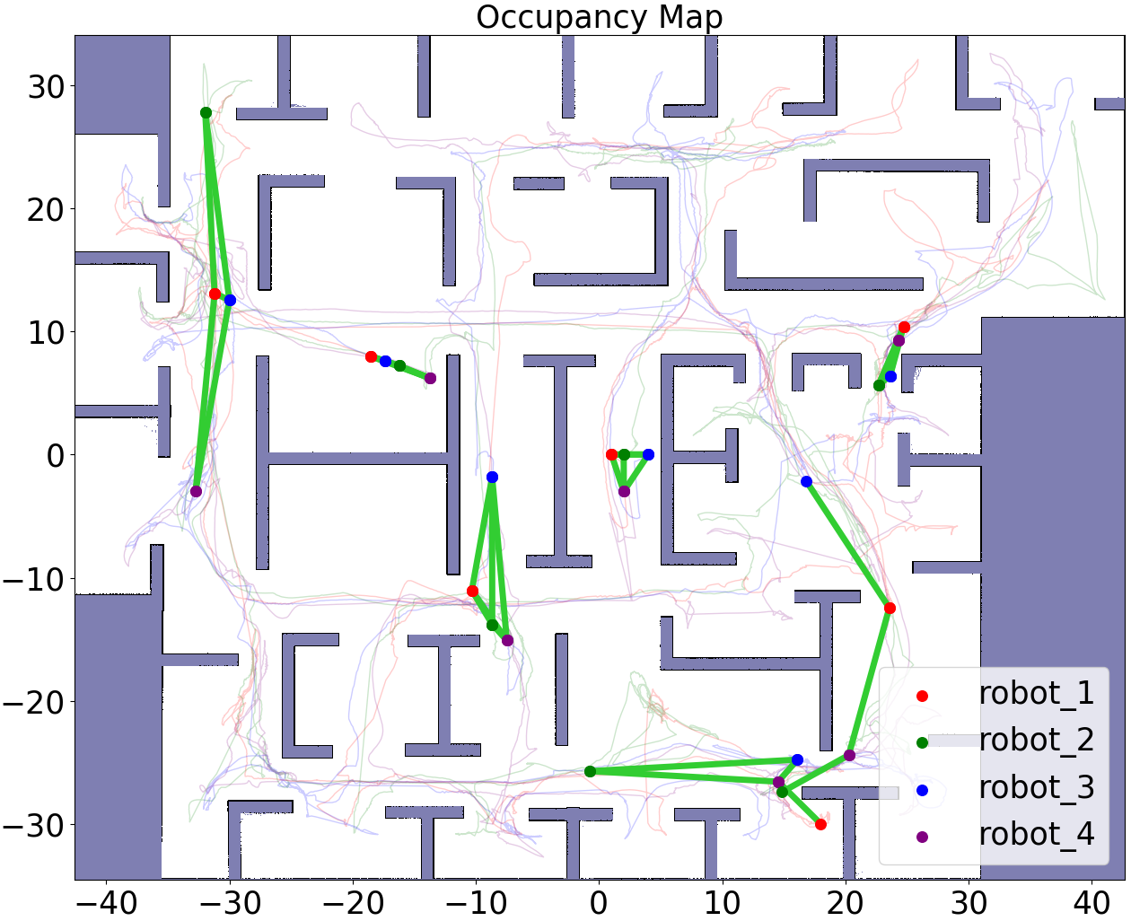
We evaluate the multi-robot connectivity maintenance of the proposed methods during the exploration of complex unknown environments, as shown in Fig. 6. The environments are filled with sharp turns and dense walls, making it challenging for robots to maintain LoS. Despite this, our method successfully maintains LoS-connectivity between robots throughout the exploration, as verified by the positive Fiedler eigenvalue $\lambda_{2}$ in Fig. 7(b). The satisfaction of constraints (C1, C2, C3) is also illustrated by the robots’ exploration trajectories and their connectivity graphs over time in Fig. 6. Furthermore, we quantitively compare the connectivity velocity $\boldsymbol{u}^{\text{c}}_{i}$ and navigation velocity $\boldsymbol{u}^{\text{n}}_{i}$ under varying Fiedler eigenvalue $\lambda_{2}$. As shown in Fig. 7(a) and (b), when $\lambda_{2}$ approaches zero, the connectivity velocity grows unbounded while the navigation velocity $\boldsymbol{u}_{i}^{\text{n}}$ is bounded as in Fig. 7(c), hence the combined velocity commands are dominated to maintain the connectivity. The role-based scaling of the navigation velocity is shown in Fig. 7 (c) and (d), where the leading robot has a larger magnitude of the navigation velocity to resolve deadlocks when two robots move in opposite directions.

We also demonstrate the proposed method in the real-world, as shown in Fig. 6(c), where three DJI Tello Mini Drones with simulated 2D laser with 360 degrees of FoV are deployed. One drone follows a sequence of user-specified goals while the others move to maintain LoS connectivity. The results show that the robots can always maintain LoS connectivity when navigating in an unknown environment with obstacles. More experiments and details can be found in the attached video.

Multi-sensor fusion: Our method accepts different LiDAR configurations, where multiple point cloud measurements can be fused after calibration into a single, larger point cloud to directly determine the visible region for a robot with a larger field of view, without additional adaptation.

Kinematic model of robots: Although we assume a first-order kinematic model as in Eq. (2), the velocity commands $\boldsymbol{u}^{\text{c}}_{i}$ and $\boldsymbol{u}^{\text{n}}_{i}$ can be mapped to control mobile robots with unicycle models using near-identity diffeomorphism as in [25].

Note we adopted the formulations in [11] to derive the communication radius (C1) and collision avoidance constraints (C3) in this work.

References

- [1] Y. Tian, K. Liu, K. Ok, L. Tran, D. Allen, N. Roy, and J. P. How, “Search and rescue under the forest canopy using multiple uavs,” The International Journal of Robotics Research, vol. 39, no. 10-11, pp. 1201–1221, 2020.
- [2] X. Xu, M. Cao, S. Yuan, T. H. Nguyen, T.-M. Nguyen, and L. Xie, “A cost-effective cooperative exploration and inspection strategy for heterogeneous aerial system,” in 2024 IEEE 18th International Conference on Control & Automation (ICCA), pp. 673–678, 2024.
- [3] R. Bai, H. Guo, W.-Y. Yau, and L. Xie, “Graph-based slam-aware exploration with prior topo-metric information,” IEEE Robotics and Automation Letters, vol. 9, no. 9, pp. 7597–7604, 2024.
- [4] G. Shi, I. E. Rabban, L. Zhou, and P. Tokekar, “Communication-aware multi-robot coordination with submodular maximization,” in 2021 IEEE International Conference on Robotics and Automation (ICRA), pp. 8955–8961, 2021.
- [5] C. Cao, H. Zhu, Z. Ren, H. Choset, and J. Zhang, “Representation granularity enables time-efficient autonomous exploration in large, complex worlds,” Science Robotics, vol. 8, no. 80, p. eadf0970, 2023.
- [6] D. M. S. Tan, Y. Ma, J. Liang, Y. C. Chng, Y. Cao, and G. Sartoretti, “Ir 2: Implicit rendezvous for robotic exploration teams under sparse intermittent connectivity,” in 2024 IEEE/RSJ International Conference on Intelligent Robots and Systems (IROS), pp. 13245–13252, IEEE, 2024.
- [7] V. S. Varadharajan, D. St-Onge, B. Adams, and G. Beltrame, “Swarm relays: Distributed self-healing ground-and-air connectivity chains,” IEEE Robotics and Automation Letters, vol. 5, no. 4, pp. 5347–5354, 2020.
- [8] J. Liu and G. Hu, “Relative localization estimation for multiple robots via the rotating ultra-wideband tag,” IEEE Robotics and Automation Letters, vol. 8, no. 7, pp. 4187–4194, 2023.
- [9] F. Amigoni, J. Banfi, and N. Basilico, “Multirobot exploration of communication-restricted environments: A survey,” IEEE Intelligent Systems, vol. 32, no. 6, pp. 48–57, 2017.
- [10] L. Xia, B. Deng, J. Pan, X. Zhang, P. Duan, B. Zhou, and H. Cheng, “RELINK: Real-time line-of-sight-based deployment framework of multi-robot for maintaining a communication network,” IEEE Robotics and Automation Letters, vol. 8, no. 12, pp. 8152–8159, 2023.
- [11] P. Robuffo Giordano, A. Franchi, C. Secchi, and H. H. Bülthoff, “A passivity-based decentralized strategy for generalized connectivity maintenance,” The International Journal of Robotics Research, vol. 32, no. 3, pp. 299–323, 2013.
- [12] T. Nestmeyer, P. Robuffo Giordano, H. H. Bülthoff, and A. Franchi, “Decentralized simultaneous multi-target exploration using a connected network of multiple robots,” Autonomous robots, vol. 41, pp. 989–1011, 2017.
- [13] Y. Chen and M. Guo, “Multi-UAV deployment in obstacle-cluttered environments with LOS connectivity,” Arxiv, 2023. arXiv: 2308.12117 [cs.RO].
- [14] Y. Yang, Y. Lyu, and W. Luo, “Minimally constrained multi-robot coordination with line-of-sight connectivity maintenance,” in 2023 IEEE international conference on robotics and automation (ICRA), pp. 7684–7690, 2023.
- [15] G. A. Hollinger and S. Singh, “Multirobot coordination with periodic connectivity: Theory and experiments,” IEEE Transactions on Robotics, vol. 28, no. 4, pp. 967–973, 2012.
- [16] E. Stump, N. Michael, V. Kumar, and V. Isler, “Visibility-based deployment of robot formations for communication maintenance,” in 2011 IEEE international conference on robotics and automation, pp. 4498–4505, 2011.
- [17] A. Dutta, A. Ghosh, and O. P. Kreidl, “Multi-robot informative path planning with continuous connectivity constraints,” in 2019 International Conference on Robotics and Automation (ICRA), pp. 3245–3251, May 2019.
- [18] M. Li, Y. Jie, Y. Kong, and H. Cheng, “Decentralized global connectivity maintenance for multi-robot navigation: a reinforcement learning approach,” in 2022 international conference on robotics and automation (ICRA), pp. 8801–8807, 2022.
- [19] M. Fiedler, “Algebraic connectivity of graphs,” Czechoslovak mathematical journal, vol. 23, no. 2, pp. 298–305, 1973.
- [20] S. Katz, A. Tal, and R. Basri, “Direct visibility of point sets,” in ACM SIGGRAPH 2007 papers, pp. 24–es, 2007.
- [21] T. Liu, Q. Wang, X. Zhong, Z. Wang, C. Xu, F. Zhang, and F. Gao, “Star-convex constrained optimization for visibility planning with application to aerial inspection,” in 2022 IEEE International Conference on Robotics and Automation (ICRA), pp. 7861–7867, 2022.
- [22] P. Yang, R. A. Freeman, G. J. Gordon, K. M. Lynch, S. S. Srinivasa, and R. Sukthankar, “Decentralized estimation and control of graph connectivity for mobile sensor networks,” Automatica, vol. 46, no. 2, pp. 390–396, 2010.
- [23] F. Yang, C. Cao, H. Zhu, J. Oh, and J. Zhang, “FAR Planner: Fast, attemptable route planner using dynamic visibility update,” in 2022 IEEE/RSJ International Conference on Intelligent Robots and Systems (IROS), pp. 9–16, 2022.
- [24] K. Konolige, G. Grisetti, R. Kümmerle, W. Burgard, B. Limketkai, and R. Vincent, “Efficient sparse pose adjustment for 2d mapping,” in 2010 IEEE/RSJ International Conference on Intelligent Robots and Systems (IROS), pp. 22–29, 2010.
- [25] S. Wilson, P. Glotfelter, L. Wang, S. Mayya, G. Notomista, M. Mote, and M. Egerstedt, “The robotarium: Globally impactful opportunities, challenges, and lessons learned in remote-access, distributed control of multirobot systems,” IEEE Control Systems Magazine, vol. 40, no. 1, pp. 26–44, 2020.
Appendix
VIII-A Formulation of Communication and Collision Avoidance Constraints