Reconstructing G-inflation: From the attractors $n_{S}(N)$ and $r(N)$

It is well known that during the dynamic evolution of the early universe, it presented a period of rapid growth called inflationary stage or merely inflation R1 ; R102 ; R103 ; Rin . The inflationary universe gives an elegant solutions to long standing cosmological problems present in the standard hot big bang model. Nevertheless, inflation not only solves the problems of the hot big bang, but also gives account of the Large-Scale Structure (LSS) R2 ; R203 , together with a causal description of the anisotropies observed in the Cosmic Microwave Background (CMB) radiation of the early universeastro ; Hinshaw:2012aka ; Ade:2013zuv ; Planck2015 ; Ob2 ; DiValentino:2016foa .

In the context of the different models that give account of the dynamical evolution of an inflationary universe, we can stand out one general class of inflationary models where the inflation is driven by a minimally coupled scalar field. In the literature these models are called the Galilean inflationary models or simply G-inflation and its generalization, known as G${}^{2}-$inflation which also corresponds to a subclass of the Horndeski theoryHo , was developed in Ref.Kobayashi:2011nu . In this context, the inclusion of the canonical and non-canonical scalar field in the model of G-inflation, is known as kinetic gravity braiding modelG1 ; G2 . From the observational point the view, the detection of gravitational waves by GW170817 and the $\gamma-$ray burst TheLIGOScientific:2017qsa ; Monitor:2017mdv ; GBM:2017lvd give a strong constrain on the speed gravitational waves. In this context, the G-model is consistent with the GW170817, since the speed gravitational waves is equal to the speed of light. Thus, the Galilean action includes an extra term of the form $G(\phi,X)\square\phi$ to the standard action, but this term on the action does not modify the speed gravitational waves and it is equivalent to the speed of light G1 ; G2 . We should also mention that the field equations still have derivatives only up to second order, see Ref.Nic . In this way, different cosmological models have been developed in the framework of G-inflation. In particular, assuming the slow roll approximation and considering some effective potentials G-inflation was studied in Ref.288 . In relation to the Higgs field, the model of Higgs G-inflation viewed as a modification of the standard Higgs inflation, in which the function $G(\phi,X)\propto\phi X$, was developed in Ref.289a , see also289 . In this modified gravity, the specific case in which the effective potential $V(\phi)=$ constant together with the slow roll approximation, is known as ultra slow roll G-inflation and it was studied in Ut . For the case in which the scalar potential is of the power-law type was studied in Ref.Pw . The model of warm inflation and its thermal fluctuations in the context of G-inflation was developed in Ref.Herrera:2017qux . The reheating mechanism in this model was studied in Ref.Br and from string gas cosmology in Ref.agr , see alsoReh2 ; DE1 ; DE2 ; Ka .

On the other hand, the idea of the reconstruction of the physical variables present on the background dynamics of inflationary models, from observational parameters such as the scalar spectrum, scalar spectral index $n_{S}$ and the tensor to scalar ratio $r$, have been studied by several authorsH1 ; H2 ; H3 ; H4 ; M ; Chiba:2015zpa ; H5 . In this context, a reconstruction mechanism to obtain the physical variables in the inflationary stage considering the slow roll approximation, is though of the parametrization of the cosmological observables $n_{S}(N)$ and $r(N)$ or commonly called attractors, in which the parameter $N$ denotes the number of e-folds.

From the observational point of view, the scalar spectral index $n_{S}$, is well supported by the parametrization in terms of the number of e-fonds $N$, given by the attractor $n_{S}\sim 1-2/N$ for large $N$, in which the number $N\simeq 50-70$ at the end of the inflationary scenario from the results of Planck and BICEP2-Keck Array Collaborations Planck2015 ; Ob2 . In the framework of the General Relativity (GR), different models can be reconstructed considering the parametrization or attractor $n_{S}(N)\sim 1-2/N$ (for large $N\sim\,\mathcal{O}(10^{2})$), to name of few we have; the hyperbolic tangent model or simply the T-model T , E-modelE , $R^{2}$-modelR102 , the chaotic inflationary modelR103 , the Higgs inflation Higgs ; Higgs2 , etc. In the context of warm inflation and its reconstruction was necessary to introduce the attractors $n_{S}(N)$ and $r(N)$ (unlike cold inflation), in order to build the scalar potential and the dissipation coefficient in terms of the scalar field Herrera:2018cgi .

Another methodology used in the literature in order to reconstruct the scalar potential, scalar spectral index and the tensor to scalar ratio is by means of the slow-roll parameter $\epsilon(N)$, as function of the number of e-folds $N$ Huang:2007qz ; M ; Gao:2017owg ; M . Also, the use of two slow roll parameters $\epsilon(N)$ and $\eta(N)$, for the reconstruction of the scalar potential and spectral index was assumed in Ref.Roest:2013fha , see also Refs.N1 ; N2 .

The goal of this investigation is to reconstruct the Galilean inflationary model or G-inflation, given the parametrization of the scalar spectral index and the tensor to scalar ratio, in terms of the number of e-folds. In this sense, we investigate how the Galilean inflationary model in which the function $G(\phi,X)$, is given by $G(\phi,X)=g(\phi)\,X$, modifies the reconstructions of the scalar potential $V(\phi)$ and the coupling parameter $g(\phi)$, from the attractor point $n_{S}(N)$ and $r(N)$. Thus, we will determine the structure of the function $g(\phi)$ and in particular of $V(\phi)$, in order to in account of the observables $n_{S}$ and the ratio $r$ given by the observations.

By considering the domination of the Galilean effect, we develop a general formalism in order to obtain the effective potential $V$ and coupling parameter $g$, from the parametrization of the cosmological attractors $n_{S}(N)$ and $r(N)$, under the slow roll approximation.

For the application of the developed formalism, we will study different examples for the attractor point $n_{S}(N)-r(N)$. From these attractors, we will reconstruct the effective potential $V(\phi)$ and the coupling parameter $g(\phi)$ in terms of the scalar field $\phi$. Also, we will obtain different constraints on the parameters present in the reconstruction.

The outline of the paper is as follows: The next section we give a brief description of the model of G-inflation. Here, the background dynamics and cosmological perturbations are presented. In the section III, we develop a general formalism in order to reconstruct the scalar potential and coupling parameter in function of the attractors $n_{S}(N)$ and $r(N)$, respectively. In section IV we apply the method for different examples of $n_{S}(N)$ and $r(N)$ so as to construct the effective potential $V(\phi)$ and the coupling $g(\phi)$ in terms of the scalar field $\phi$. Finally, in section V we give our conclusions. We chose units so that $c=\hbar=8\pi=1$.

In this section we give a brief description of the model of G-inflation. We start with the 4-dimensional action for the Galilean model given by

where $g_{4}$ denotes the determinant of the space-time metric $g_{\mu\nu}$, $R$ is the Ricci scalar and the quantity $X$ corresponds to $X=-g^{\mu\nu}\partial_{\mu}\phi\partial_{\nu}\phi/2$, where $\phi$ denotes the scalar field. The quantities $K$ and $G$ are arbitrary functions of $X$ and the scalar field $\phi$, respectively. Here, the quantity $M_{p}$ corresponds to the Planck mass.

By assuming a spatially flat Friedmann Robertson Walker (FRW) metric, along with a scalar field homogeneous in which $\phi=\phi(t)$, the Friedmann equation can be written as

Here, the parameter $H=\frac{\dot{a}}{a}$ denotes the Hubble rate, $a$ corresponds to the scale factor and $\rho$ is the energy density. In the following, the dots denote differentiation with respect to the time and the quantity $\kappa=1/M_{p}^{2}$.

From the action (1), we can identify that the energy density and the pressure associated to the scalar field $\phi$ are given by G1 ; G2

and

respectively. In the following, we will assume that the notation $K_{X}$ denotes $K_{X}=\partial K/\partial X$, $G_{\phi}$ corresponds to $G_{\phi}=\partial G/\partial\phi$, $K_{XX}=\partial^{2}K/\partial X^{2}$, etc.

In this framework, the continuity equation for the energy density $\rho$ can be written as $\dot{\rho}+3\,H\,(\rho+p)=0,$ or equivalently

Here, we have used Eqs.(3), and (4).

In particular, for the special cases in which $K=X-V(\phi)$ and $G=0$, in which $V(\phi)$ corresponds to the effective potential, we recovered the standard General Relativity (GR).

In order to study the reconstruction for the G-model, we will analyze the special case in which the functions $K(\phi,X)$ and $G(\phi,X)$ are given by

respectively. Here, $g(\phi)$ is a function that depends exclusively on the scalar field $\phi$.

From Refs.G1 ; G2 , we will assume the slow roll approximation. In this context, the potential $V(\phi)$ dominates over the quantities $X$, $|G_{X}H\dot{\phi}^{3}|$ and $|G_{\phi}X|$, wherewith the energy density $\rho_{\phi}\sim V(\phi)$ and then the Friedmann equation (2) becomes

Introducing the slow-roll parameters $\epsilon_{1}$, $\epsilon_{2}$, $\epsilon_{3}$ and $\epsilon_{4}$ given by G2

then the Eq.(5) can be rewritten as

Here, we have used the functions given by Eq.(6) and the slow roll parameters given by Eq.(8).

By considering that the slow-roll parameters $\epsilon_{1}$, $|\epsilon_{2}|$, $|\epsilon_{3}|$, $|\epsilon_{4}|\ll 1$, then the Eq.(9) is reduced to

Here, we mention that in relation to the slow roll equation (10), we have two limiting instances. The situation in which $|{\cal{A}}|\ll 1$ corresponds to the standard equations of GR in the framework of slow roll inflation. Instead, the inverse case in which $|{\cal{A}}|\gg 1$, the Galileon effect changes the dynamic equation of the scalar field $\phi$ and hence the dynamics of inflationary model. In this context, we are interested in the latter situation in which the Galileon effect modifies the dynamics of the G-model and its reconstruction. Thus, $3H\dot{\phi}{\cal{A}}\simeq-V_{\phi}$ and then $9H^{2}\dot{\phi}^{2}\simeq(V_{\phi}/g)$ suggesting that the ratio $(V_{\phi}/g)>0$. Therefore, in the case in which $V_{\phi}>0$ then the quantity $g>0$ and vice versa. In the following we shall take $V_{\phi}>0$ and $g>0$.

Typically, if the scalar field roll down potential, then the velocity of the scalar field can be written as

Here, we have considered Eq.(7). Also, we note that the parameter ${\cal{A}}>0$, since we have assumed that $\dot{\phi}<0$.

In relation to the expansion, we define the number of e-folding $N$ in order to give a measure of the inflationary expansion. In this way, we assume two different values of cosmological times $t$ and $t_{e}$. Here, the time $t_{e}$ denotes the end of inflationary epoch. Thus, the number of e-folds $N$ in the limit in which $1\ll|{\cal{A}}|$ is given by

On the other hand, the cosmological perturbations together with the scalar and tensor spectrums were obtained in Refs.Kobayashi:2011nu ; GG1 ; GG2 ; Ohashi:2012wf for the model of G-inflation. In this sense, from the action (1), the amplitude of scalar perturbations ${\cal{P_{S}}}$ generated during the inflationary epoch for a flat space and assuming the slow roll approximation we have

Because the scalar spectral index $n_{S}$ is defined as $n_{S}=d\ln{\cal{P_{S}}}/d\ln k$, then from Eq.(13) the index $n_{S}$ in terms of the standard slow roll parameters can be written as

where the standard parameters $\epsilon$ and $\eta$ are defined as

Note that in the limit $g\rightarrow 0$ (or equivalently ${\cal{A}}\rightarrow 0$), the spectral index given by Eq.(14) coincides with the GR in which $n_{S}-1\simeq-6\epsilon+2\eta$. By assuming the limit in which $|{\cal{A}}|\gg 1$, the scalar spectral index reduces to

On the other hand, in relation to the tensorial perturbations, the amplitude of the tensor mode was determined in refs.Kobayashi:2011nu ; GG1 ; GG2 ; Ohashi:2012wf , and then the tensor spectrum ${\cal{P_{T}}}$ is defined as ${\cal{P_{T}}}\simeq(2\kappa^{2}V/3\pi^{2})$. In this form, the tensor to scalar ratio $r$ in the framework of G-inflation can be written as

One again, note that in the limit ${\cal{A}}\rightarrow 0$ ( or equivalently $g\rightarrow 0$), the ratio $r$ coincides with that corresponding to GR in which $r=16\epsilon$.

Taking the limit $|{\cal{A}}|\gg 1$, the tensor to scalar ratio $r$ results

In the following we will analyze the reconstruction of the effective potential $V(\phi)$ and the coefficient $g(\phi)$ in the framework of G- inflation. In order to realize the reconstruction we will assume the limit $1\ll|{\cal{A}}|$, together with an attractor point from the index $n_{S}(N)$ and the ratio $r(N)$ on the $r-n_{S}$ plane.

In this section we develop the method to follow in order to reconstruct, the scalar potential $V(\phi)$ and the coupling parameter $g(\phi)$, assuming the scalar spectral index $n_{S}(N)$ and the tensor to scalar ratio $r(N)$ as attractors. In order to reconstruct analytically the potential $V$ and the coupling parameter $g$, we shall take the limit $|{\cal{A}}|\gg 1$. Following Refs.Chiba:2015zpa ; Herrera:2018cgi , we rewrite the spectral index and the tensor to scalar ratio given by Eqs.(16) and (18), in terms of the number of e-folds $N$ and its derivatives. Thus, from these relations and giving $n_{S}=n_{S}(N)$ and $r=r(N)$, we should find the potential $V$ and the coupling parameter $g$ as a function of the number $N$. Later, with the help of Eq.(12) we should obtain the e-folding $N$ in terms of the scalar field $\phi$ in order to reconstruct finally, the scalar potential $V(\phi)$ and the coupling parameter $g(\phi)$, respectively.

In this sense, we begin by rewriting the standard slow roll parameters as a function of the number of e-folds, taking into account that

then we get

In the following, we will assume the subscript $V_{\,N}=dV/dN$, $V_{NN}$ to $V_{NN}=d^{2}V/dN^{2}$, $g_{{}_{N}}=dg/dN$ etc.

Similarly for $V_{\phi\phi}$ we get

In this form, the standard slow roll parameters $\epsilon$ and $\eta$ are rewritten as

and

respectively.

Now, the relationship between the e-folds $N$ and the scalar field $\phi$, from Eq.(12) can be written as

In this context, by considering Eqs.(16), (21) and (22) we find that the scalar spectral index $n_{S}$ can be rewritten in terms of the e-folding $N$, such that

or equivalently

From Eq.(18) we obtain that the tensor to scalar ratio becomes

Here, we have considered that the function $\cal{A}$ can be rewritten as ${\cal{A}}=-3gH\dot{\phi}=\sqrt{g}\,(\kappa\,V\,\sqrt{g}\,V_{\,N})^{1/3}.$ Also, we note that in the context of the reconstruction and assuming ${\cal A}\gg 1$, the ratio $r$ given by Eq.(25) does not depend of the parameter $g$. Here, we noted that this ratio $r$ is similar to the one obtained in the standard GR, where $r=8V_{N}/V$, see Ref.Chiba:2015zpa .

Now, from Eqs.(24) and (25) we obtain that the effective potential in terms of the e-folding $N$ results

and the coupling parameter $g(N)$ becomes

Here, we emphasize that the potential $V(N)$ depends only of the tensor to scalar ratio $r(N)$.

In fact, the Eqs.(23), (26) and (27) are the fundamental equations in order to reconstruct of the effective potential $V(\phi)$ and the parameter $g(\phi)$, giving the attractors $n_{S}(N)$ and $r(N)$, respectively.

In the following we will study some specific examples in order to reconstruct the scalar potential $V(\phi)$ and coupling parameter $g(\phi)$, from the cosmological parameters or attractors $n_{S}(N)$ and $r(N)$, respectively.

In order to apply the formalism of above, we shall first consider the simplest example for the attractors $n_{S}(N)$ and $r(N)$, so as to reconstruct analytically the effective potential $V(\phi)$ and coupling parameter $g(\phi)$. In this sense and following Refs.T ; Chiba:2015zpa , we assume that the spectral index in terms of the number of e-folds is given by

and the tensor to scalar ratio as

where $\alpha>0$ corresponds to a dimensionless constant. We mention that in the framework of GR, for the chaotic model (in which $V(\phi)\propto\phi^{2}$) R103 , the parametrization in terms of $N$ of the scalar index is given by Eq.(28), where the value of the parameter $\alpha=8$, i.e., $r(N)=8/N$, see Ref.Chiba:2015zpa . In particular if we consider that the number $N$ before the end of inflationary scenario occurs at $N\simeq 60$, then the tensor to scalar ratio given by Eq.(29) is well corroborated by observational data when the constant $\alpha<4.2$. Here, we have used that the ratio $r<0.07$ from BICEP2 and Keck Array CollaborationsOb2 .

From the attractor given by Eq.(29), we find that the effective potential (26) results

where $V_{0}>0$ corresponds to the integration constant (with units of $M_{p}^{4}$). By utilizing the spectral index (28), we obtain that the integral expression $\exp[\int(n_{s}-1)]dN=\beta/N^{2}$, in which $\beta$ denotes an integration constant (with units of $M_{p}^{-11/2}$ or $\kappa^{11/4}$). In this form, we obtain that the coupling parameter $g(N)$ in terms of e-folds from Eq.(27) can be written as

By using Eqs.(30) and (31), we find that the parameter $\cal{A}$ in terms of the number of e-folds results

From the condition in which predominate the Galileon effect, such that ${\cal{A}}\gg 1$, then from Eq.(32) we find a lower limit for the parameter $\beta$ given by $\beta\gg\frac{\alpha^{3/4}N^{\frac{5C-6\alpha}{4C}}}{(CV_{0}^{2}\kappa^{1/3})^{3/4}}$. In particular for $N=60$, $\alpha=4$ and assuming that the potential at the end of inflation $V(N=60)\simeq 10^{-11}M_{p}^{4}$ (in which $V_{0}\simeq 1.5\times 10^{-12}M_{p}^{4}$), we find that the lower bound for the parameter $\beta$ is given by $\beta\,M_{p}^{11/2}\simeq 2.9\times 10^{18}\sim\,\mathcal{O}(10^{18})$.

Now, combing Eqs.(23), (30) and (31), we find that the relationship between the e-folding $N$ and the scalar field $\phi$ results

where $\phi_{0}$ corresponds to an integration constant and the quantities $N_{0}$ and $\gamma_{1}$ are given by

respectively.

In this form, we find that the reconstruction of the effective potential $V(\phi)$ can be written as

where the quantity $\bar{V}_{0}$ is defined as $\bar{V}_{0}=V_{0}\,N_{0}$. Here, we note that the effective potential $V(\phi)$ corresponds to a power law potential in which the exponent $\frac{\alpha\,\gamma_{1}}{C}>0$. In particular for case in which the parameter $\alpha=4$, we find that the effective potential $V(\phi)\propto\phi^{0.52}$.

Analogously, from Eqs.(31) and (33), we obtain that the coupling parameter $g$ in terms of the scalar field results

where the constant $\gamma_{2}=\frac{6(C-\alpha)}{4C-3\alpha}>0$ and the quantity $\bar{g}_{0}=g_{0}\,N_{0}$. We noted that in particular if the parameter $\alpha=4$, then the power $\gamma_{2}\simeq 1.2$ and the coupling parameter $g$ decays as $g(\phi)\propto\phi^{-1.2}$. Also, we noted that for values of $\alpha\simeq 0$ (or equivalently $r\simeq 0$) and the power $\gamma_{2}\simeq 3/2$, then the coupling parameter decays as $g(\phi)\propto\phi^{-3/2}$. Also, we note that for the value $\gamma_{2}\simeq 3/2$ (or equivalently $\alpha\simeq 0$), the scalar potential $V(\phi)\sim$ constant, leading to an exponential expansion R1 . Thus, we find that the range for the parameter $\gamma_{2}$ is given by $1.1<\gamma_{2}\lesssim 3/2$.

In order to give an account of the end of inflationary stage in this reconstruction, we consider that inflation ends when the slow-roll parameter $\epsilon_{1}(\phi=\phi_{e})=-\dot{H}/H^{2}=1$ or equivalently $\ddot{a}=0$. Under slow roll approximation and considering the limit ${\cal{A}}\gg 1$, we write $\epsilon_{1}$ in terms of standard slow roll parameter $\epsilon$ as $\epsilon_{1}\simeq\frac{\epsilon}{(g\,V_{\phi})^{1/2}}$. In this way, combining Eqs.(15), (34) and (35), we obtain that the scalar field at the end of inflation becomes

Also, the condition for that inflation takes place is $\epsilon_{1}<1$ (or equivalently $\ddot{a}>0$). Thus, during inflation the scalar field is such that $\phi>\phi_{0}+\tilde{\phi_{0}}$. This results suggest that the coupling parameter $g(\phi)$ given by Eq.(35) does not present a singularity at $\phi=\phi_{0}$, during the inflationary scenario. Thus, at the end of inflation $g(\phi_{e})=\bar{g_{0}}/\tilde{\phi_{0}}^{\gamma_{2}}$ and the scalar potential $V(\phi_{e})=\bar{V_{0}}\,\tilde{\phi_{0}}^{\alpha\gamma_{1}/C}$.

Other type of the attractor for the ratio $r$ studied in the literature is given by $r=1/N(1+\xi N)$, where $\xi$ is a free parameterChiba:2015zpa ; Herrera:2018cgi , such that $\xi>-4/315$ in order to obtain from BICEP2 and Keck Array Collaborations $r<0.07$, see Ref.Ob2 . By considering this attract together with $n_{s}$ given by Eq.(28), we find a transcendental equation from Eq.(23) to express the number $N$ in terms of the field $\phi$, wherewith the reconstruction does not work.

In order to find a simple relationship between the number of e-folding $N$ and the scalar field, we consider Eq.(28) together with the attractor $r(N)$ given by

where $\xi$ corresponds to a constant (dimensionless) and it satisfies the lower bound $\xi>-0.24$, such that in particular $r(N=60)<0.07$. Note that the relation between the ratio $r$ and the scalar spectral index $n_{S}$, can be written as

Here, we have used Eqs.(28) and (36), respectively.

From Eq.(26) we find that the effective potential $V(N)$ becomes

where $C_{1}>0$ is an integration constant (with units of $M_{P}^{4}$). Note that for the case in which the parameter $\xi\gg 1/N^{1/3}$, the scalar potential $V(N)\sim C_{1}/\xi=$ constant. By using Eq.(27) we obtain that the coupling parameter $g$ in terms of the number of e-folds $N$ results

Here, we note that the coupling $g(N)$ does not depend of the constant $\xi$, only of the integration constants $\beta$ and $C_{1}$, respectively. From the condition in which predominate the Galileon effect, where ${\cal{A}}\gg 1$, we find a lower bound for the integration constants $\beta$ and $C_{1}$ given by

In particular for $N=60$ and $\xi=-0.2$ the lower limit gives $g_{0}C_{1}\sqrt{\kappa}\gg 1534$ and for the value $\xi=0.2$ corresponds to $g_{0}C_{1}\sqrt{\kappa}\gg 3419$. Also, in the special case in which the potential at the end of inflation $V(N=60)=10^{-11}M_{p}^{4}$, together with $\xi=-0.2$ we have $C_{1}\simeq 5\times 10^{-12}M_{p}^{4}$, then we find that the lower limit for the integration constant $\beta$ is given by $\beta M_{p}^{11/2}\gg\,\mathcal{O}(10^{18})$. For the case $\alpha=0.2$, we have $C_{1}\simeq 9.7\times 10^{-12}M_{p}^{4}$ and then $\beta M_{p}^{11/2}\gg 2\times 10^{18}\sim\,\mathcal{O}(10^{18})$.

On the other hand, from Eq.(23) is easy to find that the relation between $N$ and $\phi$ is given by lineal equation i.e., $N\propto\phi$. Thus, the reconstruction of the coupling parameter $g$ as a function of the scalar field is given by $g(\phi)\propto\phi^{-4/3}$. This result suggests that again the parameter $g(\phi)$ has a behavior power law with a negative power. In this point, we mention that in order to obtain the lineal relation $N\propto\phi$, we establish from Eq.(23) the condition $(V_{N}/(\kappa^{2}gV^{2}))^{1/3}=$ constant. Thus, combing Eqs.(24) and (25) together with the attractor $n_{S}$ given by Eq.(28), we obtained the tensor to scalar ratio $r$ given by Eq.(36) (or the potential Eq.(38)).

This methodology can be used for any function $F(N)$, such that $(V_{N}/(\kappa^{2}gV^{2}))^{1/3}=F(N)$. In this sense, the Eq.(23) takes of form $\int F(N)dN=\int d\phi$, being possible to choose any function $F(N)$ in order to obtain an analytical and invertible solution for $N=N(\phi)$. Subsequently, we solve the differential equation for the variable $r(N)$ (or $V(N)$ or also $g(N)$), by combining Eqs.(24), (25) and (28) for a specific function $F(N)$. In particular, for the case in which the function $F(N)=$constant, we have $N\propto\phi$, and then we found that the tensor to scalar ratio $r(N)$ is given by Eq.(36), and hence the form of the potential $V(N)$ and the coupling $g(N)$ correspond to the equations (38) and (39), respectively.

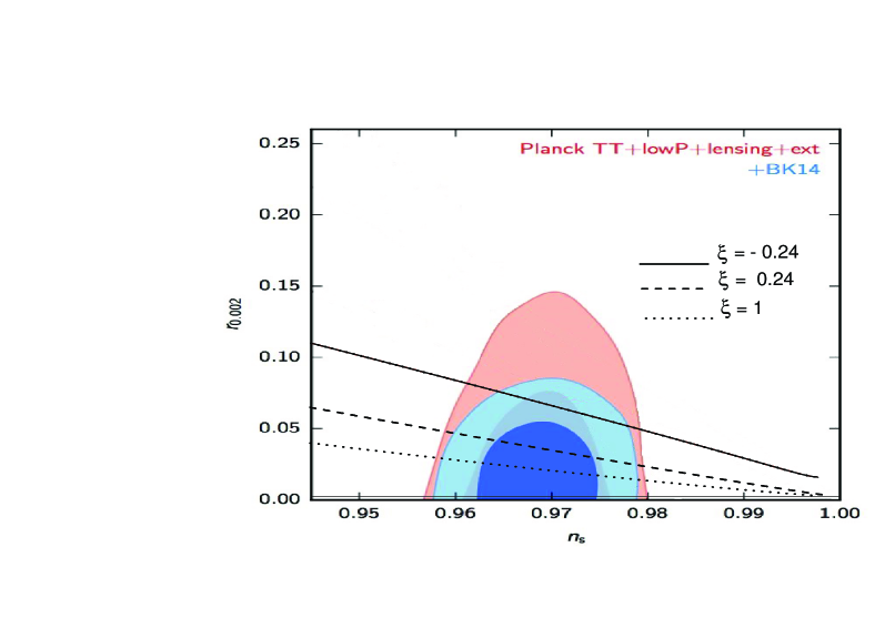
In Fig.1 we show the evolution of the ratio $g(N)/g_{0}$ on the number of e-folds $N$ (left panel) from Eq.(39) and as it decays in terms of the number of e-folds $N$ (or equivalently $\phi$, since $N\propto\phi$). In the right panel, we show the dependence of the inflationary parameters $r=r(n_{S})$ from Eq.(37). Here, we show the two-dimensional marginalized constraints (68$\%$ and 95$\%$ C.L.) on the tensor to scalar ratio $r=r(n_{s})$, derived from observational dataOb2 . In the plot we have used Eq.(37), together with three different values of the parameter $\xi$. We note that for values of $\xi>-0.241$ the relation given by Eq.(37) is well supported by the BICEP2 and Keck Array Collaborations in which $r<0.07$ and $n_{S}\simeq 0.967$ Ob2 .

In this paper we have investigated the reconstruction in the model of G-inflation, from the cosmological parameters such as the scalar spectral index $n_{S}(N)$ and the tensor to scalar ratio $r(N)$, in which $N$ denotes the number of e-folding. By assuming the domination of the Galilean term and under the slow roll approximation, we have developed a general formalism of reconstruction in which the function $G(\phi,X)=g(\phi)\,X$ .

Under this general analysis we have found from the attractor point $n_{S}(N)$ and $r(N)$, integrable expressions for the effective potential $V(N)$ and the coupling parameter $g(N)$, respectively. Curiously, in the context of the reconstruction we have found that the tensor to scalar ratio $r$ is similar to the one obtained in the GR, in which $r$ depends only of the potential and its derivative, and it does not depend of the coupling $g$.

As the simplest example and in order to find the reconstructions of the potential $V(\phi)$ and the coupling parameter $g(\phi)$, we have assumed the standard attractors given by $n_{S}-1=-2/N$ and $r=\alpha/N$, for large $N$. From these attractors, we have applied our general formalism and also we have found that both, the potential $V(N)$ and the coupling parameter $g(N)$ present a power law relation with $N$. From the condition ${\cal{A}}\gg 1$ in which predominate the Galileon term, we have obtained a lower bound for the integration constant $\beta$ given by $\beta\gg\frac{\alpha^{3/4}N^{\frac{5C-6\alpha}{4C}}}{(CV_{0}^{2}\kappa^{1/3})^{3/4}}$. In particular for the specific cases in which $N=60$, $\alpha=4$ and $V_{0}/M_{p}^{4}\sim\mathcal{O}(10^{-12})$, we have obtained that the lower limit for the constant $\beta$ results $\beta M_{p}^{11/2}\sim\mathcal{O}(10^{18})$. In this context, from the standard attractor point, we have found that the reconstruction of the scalar potential and the coupling parameter are given by Eqs.(34) and (35). Here, we have determined that the parameter $g(\phi)$ decays as $g(\phi)\propto\phi^{-\gamma_{2}}$ with $\gamma_{2}$ a positive constant.

Other, important attract in GR corresponds to $r=(N(1+\xi N))^{-1}$ together $n_{s}-1=-2/N$, here we could not find an analytical expression for $N=N(\phi)$, in order to obtain the reconstruction of $V(\phi)$ and $g(\phi)$, respectively.

Another, analytical reconstruction in the model of G-inflation corresponds to the tensor to scalar ratio $r(N)$ given by Eq.(36). Assuming that the function $F(N)=$ constant, we have find a simple relation between the number $N$ and $\phi$ given by $N\propto\phi$ and then Eq.(36). Here, we have obtained that the parameter $g$ in terms of the scalar field is given by $g(\phi)\propto\phi^{-4/3}$ and the effective potential $V(\phi)\propto\phi^{1/3}/(3+\xi^{\prime}\phi^{1/3})$. Also, in particular we have find that for the case in which the parameter $\xi\gg 1/N^{1/3}$, the scalar potential $V(\phi)$ becomes a constantR1 . In fact, by assuming the condition ${\cal{A}}(N)\gg 1$, we have obtained a lower bound for the integration constants given by Eq.(40).

Finally in this paper, we have not addressed the reconstruction to another functions $G(\phi,X)$ in the action, such as $G(\phi,X)=g(\phi)\,X^{n}$ or $g_{1}(\phi)X+g_{2}(\phi)X^{2}+..$ or other. In this sense, we hope to return to this point in the near future.