Recovering Accurate Labeling Information from Partially Valid Data for Effective Multi-Label Learning

Ximing Li^1,2 &Yang Wang^3,4,¹¹1Yang Wang is the Corresponding Author, denoted by * ¹ College of Computer Science and Technology, Jilin University, China
² Key Laboratory of Symbolic Computation and Knowledge Engineering of Ministry of Education, Jilin University, China
³ Key Laboratory of Knowledge Engineering with Big Data, Ministry of Education, Hefei University of Technology, China
⁴ School of Computer Sci & Information Engineering, Hefei University of Technology, China
liximing86@gmail.com, yangwang@hfut.edu.cn

Abstract

Partial Multi-label Learning (PML) aims to induce the multi-label predictor from datasets with noisy supervision, where each training instance is associated with several candidate labels but only partially valid. To address the noisy issue, the existing PML methods basically recover the ground-truth labels by leveraging the ground-truth confidence of the candidate label, i.e., the likelihood of a candidate label being a ground-truth one. However, they neglect the information from non-candidate labels, which potentially contributes to the ground-truth label recovery. In this paper, we propose to recover the ground-truth labels, i.e., estimating the ground-truth confidences, from the label enrichment, composed of the relevance degrees of candidate labels and irrelevance degrees of non-candidate labels. Upon this observation, we further develop a novel two-stage PML method, namely Partial Multi-Label Learning with Label Enrichment-Recovery (PML³er), where in the first stage, it estimates the label enrichment with unconstrained label propagation, then jointly learns the ground-truth confidence and multi-label predictor given the label enrichment. Experimental results validate that PML³er outperforms the state-of-the-art PML methods.

1 Introduction

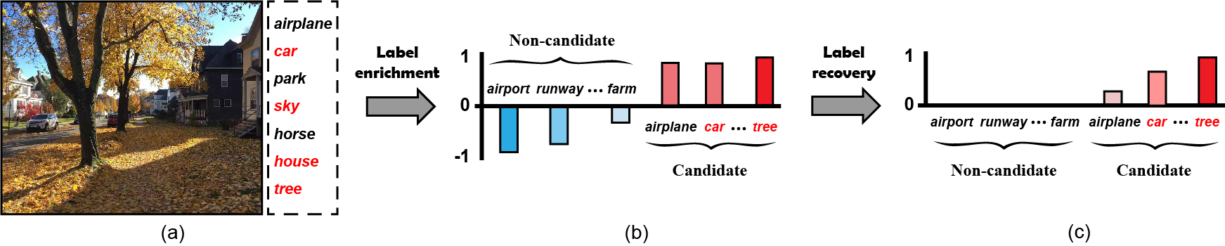
Partial Multi-label Learning (PML), a novel learning paradigm with noisy supervision, draws increasing attention from the machine learning community Fang and Zhang (2019); Sun et al. (2019). It refers to induce the multi-label predictor from PML datasets, with each training instance associated with multiple candidate labels that are only partially valid. The PML datasets are available in many real-world applications, where collecting the accurate supervision is quite expensive for many scenarios, e.g., crowdsourcing annotations. To visualize this, we illustrate a PML image instance in Fig.1(a): an annotator may roughly select more candidate labels, so as to cover all ground-truth labels but ineluctably with several irrelevant ones, imposing big challenges for learning with such noisy PML training instances.

Formally speaking, given a PML dataset ${\mathcal{D}}=\{\left(\mathbf{x}_{i},\mathbf{y}_{i}\right)\}_{i=1}^{i=n}$ with $n$ instances and $l$ labels, where $\mathbf{x}_{i}\in\mathbb{R}^{d}$ denotes the feature vector and $\mathbf{y}_{i}\in\{0,1\}^{l}$ the candidate label set of $\mathbf{x}_{i}$ . For $\mathbf{y}_{i}$ , the value of 0 or 1 represents the corresponding label to be a non-candidate or candidate label. Let $\mathbf{y}^{*}\in\{0,1\}^{l}$ denote the (unknown) ground-truth label sets of instances. Specifically, for each instance $\mathbf{x}_{i}$ , its corresponding $\mathbf{y}^{*}_{i}$ is covered by the candidate label set $\mathbf{y}_{i}$ , i.e., $\mathbf{y}^{*}_{i}\subseteq\mathbf{y}_{i}$ . Accordingly, the task of PML aims to induce a multi-label predictor $f(\mathbf{x}):\mathbb{R}^{d}\to\{0,1\}^{l}$ from $\mathcal{D}$ .

Refer to caption — Figure 1: The basic idea of PML³er. (a) An example of PML image instance annotated with 7 candidate labels, with only 4 of them are ground-truth labels, *i.e.,* the ones in red (best view in color). (b) indicates the label enrichment, *i.e.,* estimating both the relevance degrees of the candidate labels within (0,1) range, and irrelevance degrees of the non-candidate labels within (-1,0) range. (c) indicates the label recovery, *i.e.,* estimating the ground-truth confidences of candidate labels from the label enrichment. The candidate label “airplane” is more likely to be an irrelevant noisy label, since its highly correlated labels, *e.g.,* “airport” and “runway”, are with higher irrelevance degrees, to filter out the noisy candidate label.

To solve the problem, several typical attempts have been made Xie and Huang (2018); Yu et al. (2018); Fang and Zhang (2019); Sun et al. (2019), where the basic idea is to recover the ground-truth labels by leveraging the ground-truth confidence of the candidate label, i.e., the likelihood of a candidate label being a ground-truth one, and learning with it, instead of the candidate label. For example, an early framework of PML Fang and Zhang (2019) estimates the ground-truth confidences via label propagation over an instance neighbor graph, following the intuition that neighboring instances tend to share the same labels; another work Sun et al. (2019) recovered the ground-truth confidences by decomposing the candidate labels under a low-rank scheme.

Revisiting the existing PML methods, we find that they basically estimate the ground-truth confidence around candidate label annotations, but neglect the information from non-candidate labels, which potentially contributes to the ground-truth label recovery. The irrelevance degree of the non-candidate label, i.e., the degree of a non-candidate label being irrelevant with the instance, is contributive to distinguish the irrelevant noisy labels within candidate label sets, since any candidate label tends to be an irrelevant noisy one if its highly correlated labels are given higher irrelevance degrees. For example, in Fig.1(b) and (c), the candidate label “airplane” is more likely to be an irrelevant noisy label, since its highly correlated labels, e.g., “airport” and “runway”, are with higher irrelevance degrees for the example image instance.

Based on the above analysis, we propose to estimate the ground-truth confidences over both candidate and non-candidate labels. In particular, we develop a novel two-stage PML method, namely Partial Multi-Label Learning with Label Enrichment-Recovery (PML³er). On the first stage, we estimate the label enrichment, composed of the relevance degrees of candidate labels (i.e., the complementary definition of irrelevance degree) and irrelevance degrees of non-candidate ones, using an unconstrained label propagation procedure. In the second stage, we jointly train the ground-truth confidence and multi-label predictor given the label enrichment learned from the first stage. We conduct extensive experiments to validate the effectiveness of PML³er.

The contributions of this paper are summarized below:

•

We propose PML³er by leveraging both the information from candidate and non-candidate labels.
•

The PML³er estimates the label enrichment using unconstrained label propagation, and then trains the multi-label predictor with label recovery simultaneously.
•

We conduct extensive experiments to validate the effectiveness of PML³er.

2 Related Work

2.1 Partial Multi-label Learning

Abundant researches towards Partial Label Learning (PLL) have been made, where each training instance is annotated with a candidate label set but only one is valid Cour et al. (2011); Liu and Dietterich (2012); Chen et al. (2014); Zhang et al. (2017); Yu and Zhang (2017); Wu and Zhang (2018); Gong et al. (2018); Chen et al. (2018); Feng and An (2018, 2019b, 2019a); Wang et al. (2019). The core idea of PLL follows the spirit of disambiguation, i.e., identifying the ground-truth label from the candidate label set for each instance. In some cases, PLL can be deemed as a special case of PML, where the ground-truth label number is fixed to one. Naturally, PML is more challenging than PLL, even the number of ground-truth labels is unknown.

The existing PML methods mainly recover the ground-truth labels by estimating the ground-truth confidences Xie and Huang (2018); Yu et al. (2018); Fang and Zhang (2019); Sun et al. (2019). Two PML methods are proposed Xie and Huang (2018), i.e., Partial Multi-label Learning with label correlation (PML-lc) and feature prototype (PML-fp), which are upon the ranking loss objective weighted by ground-truth confidences. The other one Sun et al. (2019), namely Partial Multi-label Learning by Low-Rank and Sparse decomposition (PML-LRS), trains the predictor with ground-truth confidences under the low-rank assumption. Besides them, the two-stage PML framework Fang and Zhang (2019), i.e., PARTIal multi-label learning via Credible Label Elicitation (Particle), estimates the ground-truth confidences by label propagation, and then trains the predictor over candidate labels with high confidences only. Two traditional methods of victual Label Splitting (VLS) and Maximum A Posteriori (MAP) are used in its second stage, leading to two versions, i.e., Particle-Vls and Particle-Map.

Orthogonal to those methods, our PML³er estimates the ground-truth confidence using the label enrichment involving both candidate and non-candidate labels to recover more accurate supervision.

2.2 Learning with Label Enrichment

Learning with label enrichment, also known as label enhancement, explores richer label information, e.g., the label membership degrees of instances, to enhance the performance Gayar et al. (2006); Jiang et al. (2006); Li et al. (2015); Hou et al. (2016); Xu et al. (2018). The existing methods achieve the label enrichment using the similarity knowledge of instances by various schemes, such as fuzzy clustering Gayar et al. (2006), label propagation Li et al. (2015), manifold learning Hou et al. (2016) etc. They have been applied to the paradigms of multi-label learning and label distribution learning with accurate annotations.

Our PML³er also refers to the label enrichment, but it works on the scenario of PML under noisy supervision.

3 The PML³er Algorithm

Following the notations in Section 1, we denote $\mathbf{X}=[\mathbf{x}_{1},\cdots,\mathbf{x}_{n}]^{\top}\in\mathbb{R}^{n\times d}$ and $\mathbf{Y}=[\mathbf{y}_{1},\cdots,\mathbf{y}_{n}]^{\top}\in\{0,1\}^{n\times l}$ the instance matrix and candidate label matrix, respectively. For each instance $\mathbf{x}_{i}$ , $y_{ij}=1$ means that the $j$ -th label is a candidate label, otherwise it is a non-candidate one.

Given a PML dataset $\mathcal{D}=\{\mathbf{X,Y}\}$ , our PML³er first estimates the label enrichment, which describes the relevance degrees of candidate labels and irrelevance degrees of non-candidate ones. Specifically, for each instance $\mathbf{x}_{i}$ , we denote the corresponding label enrichment $\mathbf{\widehat{y}}_{i}=[\widehat{y}_{i1},\cdots,\widehat{y}_{il}]^{\top}$ as follows:

\widehat{y}_{ij}\in\left\{\begin{array}[]{lr}[0,1]\>,\>\>\>\>\>\>\>\>\mathbf{if}\>\>y_{ij}=1\\ [-1,0]\>,\>\>\>\>\mathbf{otherwise}\end{array}\right.\quad\quad\forall j\in[l],

(1)

referring to the example image instance in Fig.1(b). Further, we denote by $\mathbf{\widehat{Y}}=[\mathbf{\widehat{y}}_{1},\cdots,\mathbf{\widehat{y}}_{n}]^{\top}$ the label enrichment matrix. Then, PML³er induces the multi-label predictor from the enrichment version of PML dataset $\mathcal{\widehat{D}}=\{\mathbf{X,\widehat{Y}}\}$ .

We now describe the two stages of PML³er, i.e., label enrichment by unconstrained propagation and jointly learning the ground-truth confidence and multi-label predictor.

3.1 Label Enrichment by Unconstrained Propagation

In the first stage, PML³er estimates the label enrichment matrix $\mathbf{\widehat{Y}}$ . Inspired by Li et al. (2015); Fang and Zhang (2019), we develop an unconstrained label propagation procedure, which estimates the labeling degrees by progressively propagating annotation information over a weighted k-Nearest Neighbor (kNN) graph over the instances. The intuition is that the candidate and non-candidate labels with more accumulations during the kNN propagation tend to be with higher relevance degrees and lower irrelevance degrees, respectively.

We describe the detailed steps of the unconstrained label propagation procedure below.

[Step 1]: After constructing the kNN graph $\mathbf{\Omega}$ , for each instance $\mathbf{x}_{i}$ , we compute its reconstruction weight vector of kNNs, i.e., $\mathbf{v}_{i}=[v_{i1},\cdots,v_{in}]^{\top}\in\mathbb{R}^{n}$ , by minimizing the following objective:

	$\displaystyle\mathop{\mathbf{min}}\limits_{\mathbf{v}_{i}}\\|\mathbf{x}_{i}-\mathbf{X}^{\top}\mathbf{v}_{i}\\|_{2}^{2}$
	$\displaystyle\>{\rm{\mathbf{s.t.}}}\>\>v_{ij}\geq 0\quad\forall j\in\mathbf{\Omega}(\mathbf{x}_{i}),\>\>v_{ij}=0\quad\forall j\not\in\mathbf{\Omega}(\mathbf{x}_{i}),$		(2)

where $\mathbf{\Omega}(\mathbf{x}_{i})$ denotes the kNNs of $\mathbf{x}_{i}$ . This objective can be efficiently solved by any off-the-shelf Quadratic Programming (QP) solver²²2We apply the public QP solver of mosek downloaded at https://www.mosek.com/. Repeat to solve the problem of Eq.(2) for each instance, we can achieve the reconstruction weight matrix $\mathbf{V}=[\mathbf{v}_{1},\cdots,\mathbf{v}_{n}]^{\top}\in\mathbb{R}^{n\times n}$ . Then, we normalize $\mathbf{V}$ by row, i.e., $\mathbf{V}\leftarrow\mathbf{VD}^{-1}$ , where $\mathbf{D}={\rm{diag}}[d_{1},\cdots,d_{n}],\>d_{i}=\sum_{j=1}^{n}v_{ij}$ .

[Step 2]: Following the idea that the relationships of instances can be translated to their associated labels, we can enrich the labeling information by propagating over $\mathbf{\Omega}$ with $\mathbf{V}$ . Formally, we denote by $\mathbf{F}=[\mathbf{f}_{1},\cdots,\mathbf{f}_{n}]^{\top}\in\mathbb{R}_{+}^{n\times l}$ the label propagation solution, which is initialized by the candidate label matrix $\mathbf{Y}$ , i.e., $\mathbf{F}^{(0)}=\mathbf{Y}$ . Then, $\mathbf{F}$ can be iteratively updated by propagating over $\mathbf{\Omega}$ with $\mathbf{V}$ until convergence. At each iteration $t$ , the update equation is given by:

\mathbf{F}^{(t)}=\alpha\cdot\mathbf{V}^{\top}\mathbf{F}^{(t-1)}+(1-\alpha)\cdot\mathbf{F}^{(0)},

(3)

where $\alpha\in[0,1]$ is the propagation rate. To avoid overestimate non-candidate labels, we normalize each row of $\mathbf{F}^{(t)}$ :

	$\displaystyle f_{ij}^{(t)}=\mathbf{min}\left(1\>,\>\frac{f_{ij}^{(t)}-\mathbf{vmin}({\mathbf{f}_{i}^{(t)}})}{\mathbf{cvmax}(\mathbf{f}_{i}^{(t)})-\mathbf{vmin}(\mathbf{f}_{i}^{(t)})}\right),$
	$\displaystyle\quad\quad\quad\quad\quad\quad\quad\quad\quad\quad\quad\quad\quad\quad\forall i\in[n],\>\forall j\in[l],$		(4)

where $\mathbf{vmin}(\mathbf{f}_{i}^{(t)})$ denotes the minimum of $\mathbf{f}_{i}^{(t)}$ , and $\mathbf{cvmax}(\mathbf{f}_{i}^{(t)})$ the maximum over candidate labels in $\mathbf{f}_{i}^{(t)}$ .

[Step 3]: After obtaining the optimal $\mathbf{F}$ , denoted by $\mathbf{F}^{*}=[f^{*}_{ij}]_{n\times l}$ , we compute the label enrichment matrix $\mathbf{\widehat{Y}}$ as follows:

\widehat{y}_{ij}=\left\{\begin{array}[]{lr}f_{ij}^{*}\>,\>\>\>\>\>\>\>\>\>\>\>\>\mathbf{if}\>\>y_{ij}=1\\ f_{ij}^{*}-1\>,\>\>\>\>\mathbf{otherwise}\end{array}\right.\quad\forall i\in[n].\>\forall j\in[l]

(5)

For clarity, we summarize the unconstrained label propagation for $\mathbf{\widehat{Y}}$ in Algorithm 1.

Algorithm 1 Unconstrained label propagation for

\mathbf{\widehat{Y}}

1:The PML dataset

{\mathcal{D}}=\{\mathbf{X,Y}\}

, nearest neighbor number

k

and propagation rate

\alpha

;

2:The label enrichment matrix

\mathbf{\widehat{Y}}

3:Construct the kNN graph of

\mathbf{X}

, and initialize

\mathbf{F}^{(0)}

\mathbf{Y}

4:Compute

\mathbf{V}

by solving Eq.(2) for each instance, and then normalize it by row

5:While not convergence Do

6: Update

\mathbf{F}

using Eq.(3)

7: Normalize

\mathbf{F}

using Eq.(4)

8:End While

9:Compute

\mathbf{\widehat{Y}}

using Eq.(5)

Algorithm 2 Predictive model induction for PML³er

1:The enriched PML dataset

{\mathcal{\widehat{D}}}=\{\mathbf{X,\widehat{Y}}\}

, regularization parameters

\{\lambda_{1},\lambda_{2}\}

;

2:The predictive parameter matrix

\mathbf{W}

3:Initialize

\{\mathbf{C,B,W},\mathbf{\widehat{B},\Theta}\}

4:While not convergence Do

5: Update

\mathbf{C}

using Eq.(10)

6: For

t=1

N_{iter}

7: Update

\mathbf{\widehat{B},B,\Theta}

using Eqs.(13), (14) and (15)

8: End For

9: Update

\mathbf{W}

using Eq.(17)

10:End While

3.2 Jointly Learning the Ground-truth Confidence and Multi-label Predictor

In the second stage, PML³er jointly trains the ground-truth confidence matrix $\mathbf{C}=[c_{ij}]_{n\times l}\in[0,1]^{n\times l}$ and multi-label predictor given the enrichment version of PML dataset $\mathcal{\widehat{D}}=\{\mathbf{X,\widehat{Y}}\}$ .

First, we aim to recover $\mathbf{C}$ from $\mathbf{\widehat{Y}}$ by leveraging the following minimization:

	$\displaystyle\mathop{\mathbf{min}}\limits_{\mathbf{C,B}}\\|\mathbf{\widehat{Y}}-\mathbf{CB}\\|_{F}^{2}+\lambda_{1}\\|\mathbf{B}\\|_{*}$
	$\displaystyle\>\>\>\>{\rm{\textbf{s.t.}}}\>\>\>\>\mathbf{0}_{n\times l}\preceq\mathbf{C}\preceq\mathbf{Y},$		(6)

where $\mathbf{B}=[b_{ij}]_{l\times l}$ denotes the label correlation matrix, and $\mathbf{0}_{n\times l}$ the all zero matrix. Specifically for capturing local label correlations, we utilize the nuclear regularizer for $\mathbf{B}$ , i.e., $\|\mathbf{B}\|_{*}$ , with the regularization parameter $\lambda_{1}$ .

Second, we aim to train a linear multi-label predictor with $\mathbf{C}$ by leveraging a least square minimization with a squared Frobenius norm regularization:

\mathop{\mathbf{min}}\limits_{\mathbf{W}}\|\mathbf{C-XW}\|_{F}^{2}+\lambda_{2}\|\mathbf{W}\|_{F}^{2}

(7)

where $\mathbf{W}\in\mathbb{R}^{d\times l}$ is the predictive parameter matrix, and $\lambda_{2}$ the regularization parameter.

By combining Eqs.(6) and (7), we achieve the overall objective as follows:

	$\displaystyle\mathop{\mathbf{min}}\limits_{\mathbf{C,B,W}}\\|\mathbf{\widehat{Y}}-\mathbf{CB}\\|_{F}^{2}+\\|\mathbf{C-XW}\\|_{F}^{2}+\lambda_{1}\\|\mathbf{B}\\|_{*}+\lambda_{2}\\|\mathbf{W}\\|_{F}^{2}$
	$\displaystyle\>\>\>\>{\rm{\textbf{s.t.}}}\>\>\>\>\mathbf{0}_{n\times l}\preceq\mathbf{C}\preceq\mathbf{Y}$		(8)

Discussion on Recovering $\mathbf{C}$ from $\mathbf{\widehat{Y}}$ .

Referring to Eq.(6), we jointly learn the ground-truth confidence matrix $\mathbf{C}$ and label correlation matrix $\mathbf{B}$ by minimizing their reconstruction error of $\mathbf{\widehat{Y}}$ . By omitting the regularizers, it can be roughly re-expressed below:

	$\displaystyle\mathop{\mathbf{min}}\limits_{\mathbf{C,B}}\sum\nolimits_{i=1}^{n}\sum\nolimits_{j=1}^{l}\left(\widehat{y}_{ij}-\sum\nolimits_{h=1}^{l}c_{ih}b_{hj}\right)^{2}$
	$\displaystyle\>\>{\rm{\textbf{s.t.}}}\>\>\>\>c_{ij}\in[0,1],\>\>\forall y_{ij}=1;\quad c_{ij}=0,\>\>\forall y_{ij}=0$

Obviously, for each component $\widehat{y}_{ij}$ , it contributes that any $c_{ih}$ tends to be larger or smaller given larger value of $b_{hj}$ (i.e., a higher correlation between label $j$ and $h$ ), if $\widehat{y}_{ij}$ corresponds to a candidate label ( $\geq 0$ ) or a non-candidate one ( $\leq 0$ ). That is, we actually recover $\mathbf{C}$ using the information from candidate and non-candidate labels simultaneously.

3.2.1 Optimization

As directly solving the objective of Eq.(8) is intractable, we optimize the variables of interest, i.e., $\{\mathbf{C,B,W}\}$ , via alternating fashion, by optimizing one variable with the other two fixed. Repeat this process until convergence or reaching the maximum number of iterations. We describe the update equations of $\{\mathbf{C,B,W}\}$ one by one.

[Update ${\mathbf{C}}$ ] When { ${\rm{\mathbf{B,W}}}$ } are fixed, the sub-objective with respect to ${\mathbf{C}}$ can be reformulated as follows:

	$\displaystyle\mathop{\mathbf{min}}\limits_{\mathbf{C}}\\|\mathbf{\widehat{Y}}-\mathbf{CB}\\|_{F}^{2}+\\|\mathbf{C-XW}\\|_{F}^{2}$
	$\displaystyle\>\>\>{\rm{\textbf{s.t.}}}\>\>\>\>\mathbf{0}_{n\times l}\preceq\mathbf{C}\preceq\mathbf{Y}$		(9)

This optimization refers to a convex optimization, so as to achieve the following truncated update equation:

c_{ij}\leftarrow\left\{\begin{array}[]{lr}0\>,\>\>\>\>\>\>\>\>\>\>\>\>\mathbf{if}\>\>c^{\prime}_{ij}\leq 0\\ 1\>,\>\>\>\>\>\>\>\>\>\>\>\>\mathbf{if}\>\>c^{\prime}_{ij}\geq 1\\ c^{\prime}_{ij}\>,\>\>\>\>\>\>\>\>\>\mathbf{otherwise}\end{array}\right.\quad\forall i\in[n],\>\forall j\in[l],

(10)

where $\mathbf{C}^{\prime}=[c^{\prime}_{ij}]_{n\times l}$ :

\mathbf{C^{\prime}}=(\mathbf{\widehat{Y}B^{\top}}+\mathbf{XW})(\mathbf{BB^{\top}}+\mathbf{I}_{l})^{-1}

[Update ${\mathbf{B}}$ ] When { ${\rm{\mathbf{C,W}}}$ } are fixed, the sub-objective with respect to ${\mathbf{B}}$ can be reformulated as follows:

\mathop{\mathbf{min}}\limits_{\mathbf{B}}\|\mathbf{\widehat{Y}-CB}\|_{F}^{2}+\lambda_{1}\|\mathbf{B}\|_{*}

(11)

Following the spirit of Alternating Direction Method of Multipliers (ADMM) Boyd et al. (2011), we convert Eq.(11) into an augmented Lagrange problem with an auxiliary matrix $\mathbf{\widehat{B}}\in\mathbb{R}^{l\times l}$ and Lagrange parameter matrix $\mathbf{\Theta}\in\mathbb{R}^{l\times l}$ :

\mathop{\mathbf{min}}\limits_{\mathbf{\widehat{B},B,\Theta}}\|\mathbf{\widehat{Y}-C\widehat{B}}\|_{F}^{2}+\lambda_{1}\|\mathbf{B}\|_{*}+\frac{\tau}{2}\|\mathbf{B-\widehat{B}}+\frac{\mathbf{\Theta}}{\tau}\|_{F}^{2},

(12)

where $\tau$ is the penalty parameter. We perform an inner iteration to alternatively optimizing each of $\{\mathbf{\widehat{B},B,\Theta}\}$ with the other two fixed. After some simple algebra, the update equations are formulated as follows:

\mathbf{\widehat{B}}\leftarrow(2\mathbf{C}^{\top}\mathbf{C}+\tau\mathbf{I}_{l})^{-1}(2\mathbf{C}^{\top}\mathbf{\widehat{Y}}+\tau\mathbf{B}+\mathbf{\Theta})

(13)

For $\mathbf{B}$ , it can be directly solved by

\mathbf{B}\leftarrow\mathbf{SVD}_{\frac{\lambda_{1}}{\tau}}\left(\mathbf{\widehat{B}}-\frac{\mathbf{\Theta}}{\tau}\right),

(14)

where $\mathbf{SVD}_{\frac{\lambda_{1}}{\tau}}(\cdot)$ is the singular thresholding with $\frac{\lambda_{1}}{\tau}$ Cai et al. (2010). Then, for $\mathbf{\Theta}$ , it can be updated by:

\mathbf{\Theta}\leftarrow\mathbf{\Theta}+\tau(\mathbf{B-\widehat{B}})

(15)

[Update ${\mathbf{W}}$ ] When { ${\rm{\mathbf{C,B}}}$ } are fixed, the sub-objective with respect to ${\mathbf{W}}$ can be reformulated as follows:

\mathop{\mathbf{min}}\limits_{\mathbf{W}}\|\mathbf{C-XW}\|_{F}^{2}+\lambda_{2}\|\mathbf{W}\|_{F}^{2}

(16)

The problem has an analytic solution as follows:

\mathbf{W}=(\mathbf{X}^{\top}\mathbf{X}+\lambda_{2}\mathbf{I}_{d})^{-1}\mathbf{X}^{\top}\mathbf{C}

(17)

Algorithm 3 Full algorithm of PML³er

1:The PML dataset

{\mathcal{D}}=\{\mathbf{X,Y}\}

k=10

\alpha=0.5

and

\{\lambda_{1},\lambda_{2}\}

;

2:The predictive parameter matrix

\mathbf{W}

3:Compute the label enrichment matrix

\mathbf{\widehat{Y}}

using Algorithm 1

4:Optimize

\mathbf{W}

using Algorithm 2 given

{\mathcal{D}}=\{\mathbf{X,\widehat{Y}}\}

For clarity, we summarize the procedure of this predictive model induction in Algorithm 2.

3.3 PML³er Summary

We describe some implementation details of PML³er. First, following Fang and Zhang (2019), we fix the parameters of the unconstrained label propagation as: $k=10$ and $\alpha=0.05$ . Second, we empirically fix the penalty parameter $\tau$ of ADMM as 1. Third, the maximum iteration number of both ADMM loops is set to 5, as to be widely known, ADMM basically converges fast. Overall, the PML³er algorithm is outlined in Algorithm 3.

Time Complexity.

We also discuss the time complexity of PML³er. First, in the unconstrained label propagation procedure, we require $\mathcal{O}(n^{2}d^{2})$ time to construct the weighted kNN graph, and $\mathcal{O}(T_{1}n^{2}l)$ time to obtain the label enrichment matrix, referring to Eq.(3), where $T_{1}$ denotes its iteration number. Second, in predictive model induction, the major computational costs include matrix inversion and SVD, requiring roughly $\mathcal{O}(T_{2}(d^{3}+n^{2}l))$ time, where $T_{2}$ denotes the iteration number of the outer loop³³3Here, we omit the iteration numbers of inner ADMM loop for $\mathbf{B}$ , since it converges very fast.. Therefore, the total time complexity of PML³er is $\mathcal{O}(n^{2}d^{2}+T_{1}n^{2}l+T_{2}(d^{3}+n^{2}l))$ .

4 Experiment

4.1 Experimental Setup

Dataset	$n$	$d$	$l$	#AL	Domain
Genbase	662	1186	27	1.252	biology
Medical	978	1449	45	1.245	text
Arts	5000	462	26	1.636	text
Corel5k	5000	499	374	3.522	images
Bibtex	7395	1836	159	2.406	text

Table 1: Statistics of the original multi-label datasets. “#AL”: average label number of each instance.

Dataset	a	PML³er (Ours)	Particle-Map	PML-LRS	PML-fp	ML-kNN	Lift

RLoss $\bm{\downarrow}$
Genbase	50	.005 $\pm$ .002	.010 $\pm$ .002	.006 $\pm$ .002	.019 $\pm$ .006	.012 $\pm$ .003	.009 $\pm$ .003
	100	.005 $\pm$ .003	.010 $\pm$ .002	.005 $\pm$ .003	.018 $\pm$ .007	.014 $\pm$ .006	.008 $\pm$ .004
	150	.008 $\pm$ .003	.010 $\pm$ .001	.009 $\pm$ .002	.019 $\pm$ .010	.019 $\pm$ .006	.012 $\pm$ .004
	200	.007 $\pm$ .003	.009 $\pm$ .001	.010 $\pm$ .003	.014 $\pm$ .004	.017 $\pm$ .005	.012 $\pm$ .005
Medical	50	.028 $\pm$ .005	.048 $\pm$ .005	.033 $\pm$ .006	.042 $\pm$ .009	.075 $\pm$ .009	.044 $\pm$ .005
	100	.030 $\pm$ .006	.050 $\pm$ .006	.032 $\pm$ .006	.043 $\pm$ .011	.078 $\pm$ .012	.046 $\pm$ .007
	150	.034 $\pm$ .007	.054 $\pm$ .005	.035 $\pm$ .007	.042 $\pm$ .009	.094 $\pm$ .012	.055 $\pm$ .006
	200	.031 $\pm$ .005	.049 $\pm$ .004	.035 $\pm$ .007	.043 $\pm$ .015	.088 $\pm$ .012	.056 $\pm$ .008
Arts	50	.154 $\pm$ .003	.142 $\pm$ .002	.162 $\pm$ .002	.132 $\pm$ .002	.165 $\pm$ .003	.137 $\pm$ .003
	100	.162 $\pm$ .004	.152 $\pm$ .002	.170 $\pm$ .005	.131 $\pm$ .002	.166 $\pm$ .003	.143 $\pm$ .005
	150	.175 $\pm$ .002	.158 $\pm$ .003	.186 $\pm$ .003	.140 $\pm$ .004	.174 $\pm$ .005	.155 $\pm$ .003
	200	.180 $\pm$ .002	.165 $\pm$ .003	.192 $\pm$ .003	.146 $\pm$ .001	.172 $\pm$ .004	.156 $\pm$ .004
Corel5k	50	.174 $\pm$ .002	.128 $\pm$ .002	.206 $\pm$ .002	.198 $\pm$ .006	.146 $\pm$ .002	.144 $\pm$ .001
	100	.179 $\pm$ .003	.132 $\pm$ .002	.216 $\pm$ .003	.178 $\pm$ .008	.152 $\pm$ .001	.154 $\pm$ .002
	150	.185 $\pm$ .003	.134 $\pm$ .002	.230 $\pm$ .004	.169 $\pm$ .003	.156 $\pm$ .002	.164 $\pm$ .002
	200	.186 $\pm$ .002	.135 $\pm$ .002	.232 $\pm$ .003	.176 $\pm$ .005	.161 $\pm$ .003	.175 $\pm$ .003
Bibtex	50	.094 $\pm$ .002	.190 $\pm$ .004	.126 $\pm$ .003	.112 $\pm$ .004	.240 $\pm$ .002	.121 $\pm$ .003
	100	.100 $\pm$ .002	.187 $\pm$ .003	.138 $\pm$ .002	.107 $\pm$ .003	.250 $\pm$ .003	.130 $\pm$ .004
	150	.112 $\pm$ .002	.187 $\pm$ .002	.157 $\pm$ .002	.109 $\pm$ .003	.260 $\pm$ .003	.143 $\pm$ .003
	200	.116 $\pm$ .001	.189 $\pm$ .005	.165 $\pm$ .001	.111 $\pm$ .001	.266 $\pm$ .009	.145 $\pm$ .002
AP $\bm{\uparrow}$
Genbase	50	.991 $\pm$ .005	.978 $\pm$ .005	.988 $\pm$ .004	.981 $\pm$ .006	.968 $\pm$ .007	.982 $\pm$ .006
	100	.992 $\pm$ .004	.978 $\pm$ .004	.989 $\pm$ .004	.981 $\pm$ .007	.967 $\pm$ .008	.984 $\pm$ .003
	150	.988 $\pm$ .003	.978 $\pm$ .004	.979 $\pm$ .002	.976 $\pm$ .011	.958 $\pm$ .011	.979 $\pm$ .008
	200	.989 $\pm$ .003	.979 $\pm$ .003	.981 $\pm$ .005	.979 $\pm$ .006	.964 $\pm$ .014	.977 $\pm$ .011
Medical	50	.882 $\pm$ .014	.798 $\pm$ .018	.853 $\pm$ .021	.852 $\pm$ .023	.742 $\pm$ .029	.830 $\pm$ .017
	100	.881 $\pm$ .018	.791 $\pm$ .021	.861 $\pm$ .021	.855 $\pm$ .022	.741 $\pm$ .029	.822 $\pm$ .015
	150	.867 $\pm$ .022	.781 $\pm$ .024	.858 $\pm$ .018	.845 $\pm$ .019	.720 $\pm$ .033	.804 $\pm$ .006
	200	.870 $\pm$ .016	.768 $\pm$ .013	.855 $\pm$ .020	.853 $\pm$ .029	.715 $\pm$ .034	.797 $\pm$ .020
Arts	50	.598 $\pm$ .003	.528 $\pm$ .004	.588 $\pm$ .003	.577 $\pm$ .007	.488 $\pm$ .005	.595 $\pm$ .005
	100	.597 $\pm$ .004	.513 $\pm$ .004	.584 $\pm$ .005	.578 $\pm$ .005	.486 $\pm$ .005	.591 $\pm$ .007
	150	.577 $\pm$ .005	.499 $\pm$ .006	.564 $\pm$ .005	.558 $\pm$ .005	.478 $\pm$ .006	.577 $\pm$ .003
	200	.572 $\pm$ .003	.491 $\pm$ .006	.557 $\pm$ .005	.554 $\pm$ .005	.477 $\pm$ .003	.578 $\pm$ .005
Corel5k	50	.295 $\pm$ .004	.263 $\pm$ .005	.282 $\pm$ .003	.240 $\pm$ .003	.233 $\pm$ .003	.244 $\pm$ .005
	100	.293 $\pm$ .004	.260 $\pm$ .003	.276 $\pm$ .004	.242 $\pm$ .003	.229 $\pm$ .003	.217 $\pm$ .004
	150	.289 $\pm$ .004	.264 $\pm$ .005	.266 $\pm$ .003	.241 $\pm$ .003	.226 $\pm$ .003	.194 $\pm$ .003
	200	.288 $\pm$ .004	.260 $\pm$ .004	.266 $\pm$ .004	.241 $\pm$ .003	.224 $\pm$ .003	.185 $\pm$ .005
Bibtex	50	.567 $\pm$ .004	.383 $\pm$ .007	.532 $\pm$ .003	.517 $\pm$ .003	.295 $\pm$ .004	.487 $\pm$ .007
	100	.555 $\pm$ .004	.380 $\pm$ .006	.509 $\pm$ .005	.522 $\pm$ .005	.282 $\pm$ .005	.467 $\pm$ .007
	150	.536 $\pm$ .004	.369 $\pm$ .003	.476 $\pm$ .006	.519 $\pm$ .004	.270 $\pm$ .004	.448 $\pm$ .007
	200	.528 $\pm$ .006	.365 $\pm$ .004	.460 $\pm$ .005	.511 $\pm$ .006	.266 $\pm$ .005	.440 $\pm$ .007
Macro-F1 $\bm{\uparrow}$
Genbase	50	.710 $\pm$ .029	.543 $\pm$ .053	.680 $\pm$ .015	.598 $\pm$ .023	.622 $\pm$ .022	.619 $\pm$ .044
	100	.722 $\pm$ .044	.522 $\pm$ .017	.710 $\pm$ .027	.594 $\pm$ .056	.594 $\pm$ .022	.600 $\pm$ .039
	150	.649 $\pm$ .033	.536 $\pm$ .034	.618 $\pm$ .039	.603 $\pm$ .030	.540 $\pm$ .016	.566 $\pm$ .046
	200	.652 $\pm$ .054	.533 $\pm$ .019	.559 $\pm$ .033	.603 $\pm$ .026	.562 $\pm$ .058	.579 $\pm$ .039
Medical	50	.405 $\pm$ .027	.270 $\pm$ .013	.301 $\pm$ .016	.296 $\pm$ .015	.243 $\pm$ .034	.309 $\pm$ .022
	100	.363 $\pm$ .017	.254 $\pm$ .015	.314 $\pm$ .021	.320 $\pm$ .020	.235 $\pm$ .020	.293 $\pm$ .015
	150	.348 $\pm$ .026	.238 $\pm$ .006	.316 $\pm$ .013	.294 $\pm$ .014	.208 $\pm$ .016	.264 $\pm$ .010
	200	.373 $\pm$ .024	.227 $\pm$ .016	.315 $\pm$ .015	.315 $\pm$ .036	.192 $\pm$ .019	.266 $\pm$ .020
Arts	50	.244 $\pm$ .012	.201 $\pm$ .007	.220 $\pm$ .008	.159 $\pm$ .008	.123 $\pm$ .007	.249 $\pm$ .009
	100	.251 $\pm$ .012	.190 $\pm$ .004	.227 $\pm$ .006	.156 $\pm$ .004	.119 $\pm$ .008	.247 $\pm$ .006
	150	.240 $\pm$ .007	.180 $\pm$ .005	.229 $\pm$ .006	.129 $\pm$ .004	.112 $\pm$ .010	.237 $\pm$ .009
	200	.226 $\pm$ .006	.184 $\pm$ .007	.210 $\pm$ .006	.126 $\pm$ .004	.108 $\pm$ .005	.217 $\pm$ .005
Corel5k	50	.040 $\pm$ .001	.027 $\pm$ .001	.039 $\pm$ .001	.005 $\pm$ .000	.020 $\pm$ .001	.046 $\pm$ .002
	100	.038 $\pm$ .000	.028 $\pm$ .002	.038 $\pm$ .001	.004 $\pm$ .000	.020 $\pm$ .002	.040 $\pm$ .002
	150	.037 $\pm$ .001	.034 $\pm$ .002	.037 $\pm$ .001	.004 $\pm$ .000	.019 $\pm$ .002	.035 $\pm$ .002
	200	.036 $\pm$ .000	.032 $\pm$ .002	.032 $\pm$ .000	.004 $\pm$ .000	.018 $\pm$ .001	.033 $\pm$ .001
Bibtex	50	.375 $\pm$ .002	.163 $\pm$ .004	.359 $\pm$ .004	.299 $\pm$ .006	.133 $\pm$ .001	.299 $\pm$ .008
	100	.360 $\pm$ .002	.157 $\pm$ .004	.332 $\pm$ .004	.311 $\pm$ .002	.120 $\pm$ .004	.271 $\pm$ .008
	150	.340 $\pm$ .002	.146 $\pm$ .003	.296 $\pm$ .006	.306 $\pm$ .007	.109 $\pm$ .001	.247 $\pm$ .009
	200	.331 $\pm$ .004	.145 $\pm$ .005	.278 $\pm$ .004	.301 $\pm$ .002	.103 $\pm$ .005	.232 $\pm$ .010

Table 2: Experimental results (mean

\pm

std) in terms of RLoss, AP, Macro-F1, where the best performance is shown in boldface.

4.1.1 Datasets

In the experiment, we downloaded five public multi-label datasets from the mulan website⁴⁴4http://mulan.sourceforge.net/datasets-mlc.html, including Genbase, Medical, Arts, Corel5k and Bibtex. The statistics of those datasets are outlined in Table 1.

To conduct experiments under the scenario of noisy supervision, we generate synthetic PML datasets from each original dataset by randomly drawing irrelevant noisy labels. Specifically, for each instance, we create the candidate label set by adding several randomly drawn irrelevant labels with $a\%$ number of ground-truth labels, where we vary $a$ over the range $\{50,100,150,200\}$ . Besides, to avoid useless PML instances annotated with all $l$ labels, we fix each candidate label set at most $l-1$ labels. Accordingly, a total of twenty synthetic PML datasets are generated.

4.1.2 Baseline Methods

We employed five baseline methods for comparison, including three PML methods and two traditional methods of Multi-label Learning (ML). For the ML ones, we directly train them over the synthetic PML datasets by considering all candidate labels as ground-truth ones. We outline the method-specific settings below.

•

PML-fp Xie and Huang (2018): A PML method with a ranking loss objective weighted by ground-truth confidences. We utilize the code provided by its authors, and tune the parameters following the original paper. Here, the other version of Xie and Huang (2018), i.e., PML-lc, was neglected, since it performed worse than PML-fp in our early experiments.
•

Particle-Map Fang and Zhang (2019): A two-stage PML method with label propagation. We employ the public code⁵⁵5http://palm.seu.edu.cn/zhangml/files/PARTICLE.rar, and tune the parameters following the original paper. Here, the other version of Fang and Zhang (2019), i.e., Particle-Vls, was neglected, since it performed worse than Particle-Map in our early experiments.
•

PML-LRS Sun et al. (2019): A PML method with candidate label decomposition. We utilize the code provided by its authors, and tune the regularization parameters over $\{10^{i}|i=-3,\cdots,1\}$ using cross-validations.
•

Multi-Label k Nearest Neighbor (ML-kNN) Zhang and Zhou (2007): A kNN ML method. We employ the public code⁶⁶6http://palm.seu.edu.cn/zhangml/files/ML-kNN.rar implemented by its authors, and tune its parameters following the original paper.
•

Multi-label learning with Label specIfic FeaTures (Lift) Zhang and Wu (2015): A binary relevance ML method. We employ the public code⁷⁷7http://palm.seu.edu.cn/zhangml/files/LIFT.rar implemented by its authors, and tune its parameters following the original paper.

For our PML³er, the regularization parameter $\lambda_{1}$ is fixed to 1, and $\lambda_{2}$ is tuned over $\{10^{i}|i=1,2\}$ using 5-fold cross validation results.

4.1.3 Evaluation Metrics

We employed seven evaluation metrics Zhang and Zhou (2014), including Subset Accuracy (SAccuracy), Hamming Loss (HLoss), One Error (OError), Ranking Loss (RLoss), Average Precision (AP), Macro Averaging F1 (Macro-F1), Micro Averaging F1 (Micro-F1), where both instance-based and label-based metrics are covered. For SAccuracy, AP, Macro-F1 and Micro-F1, the higher value is better, while for HLoss, OError and RLoss, a smaller value is better.

Baseline Method	SAccuracy	HLoss	OError	RLoss	AP	Macro-F1	Micro-F1	Total
Particle-Map	20/0/0	16/4/0	20/0/0	12/0/8	20/0/0	20/0/0	20/0/0	128/4/8
PML-LRS	17/2/1	9/11/0	20/0/0	17/3/0	20/0/0	18/2/0	20/0/0	121/18/1
PML-fp	20/0/0	18/2/0	19/1/0	11/1/8	20/0/0	20/0/0	20/0/0	128/4/8
ML-kNN	20/0/0	20/0/0	20/0/0	14/0/6	20/0/0	20/0/0	20/0/0	134/0/6
Lift	19/0/1	17/3/0	17/2/1	12/0/8	18/1/1	17/0/3	19/1/0	119/7/14

Table 3: Win/tie/loss counts of pairwise

t

-test (at 0.05 significance level) between PML³er and each comparing approach.

4.2 Experimental Results

For each PML dataset, we randomly generate five 50%/50% training/test splits, and evaluate the average scores ( $\pm$ standard deviation) of comparing algorithms. Due to the space limitation, we only present detailed results of RLoss, AP and Macro-F1 in Table 2, while the observations of other metrics tend to be similar. First, we can observe that PML³er outperforms other three PML methods in most cases, where PML³er dominates the scenarios of AP and Macro-F1 on different noise levels. Especially, the performance gain over Particle-Map indicates that using the information from non-candidate labels is beneficial for PML. Besides, we can see that PML³er significantly performs better than the two traditional ML methods in most cases, since they directly use noisy candidate labels for training.

Additionally, for each PML dataset and evaluation metric, we conduct a pairwise t-test (at 0.05 significance level) to examine whether PML³er is statistically different to baselines. The win/tie/loss counts over 20 PML datasets and 7 evaluation metrics are presented in Table 3. We can observe that PML³er significantly outperforms the PML baseline methods Particle-Map, PML-LRS and PML-fp in $91.4\%$ , $86.4\%$ and $91.4\%$ cases, and also outperforms the two traditional MLL methods ML-kNN and Lift in $95.7\%$ and $85\%$ cases. Besides, on the results of evaluation metrics, PML³er achieves significantly better scores. For example, the SAccuracy, OError, AP, Macro-F1 and Micro-F1 of PML³er are better than all comparing algorithms in $95\%$ cases.

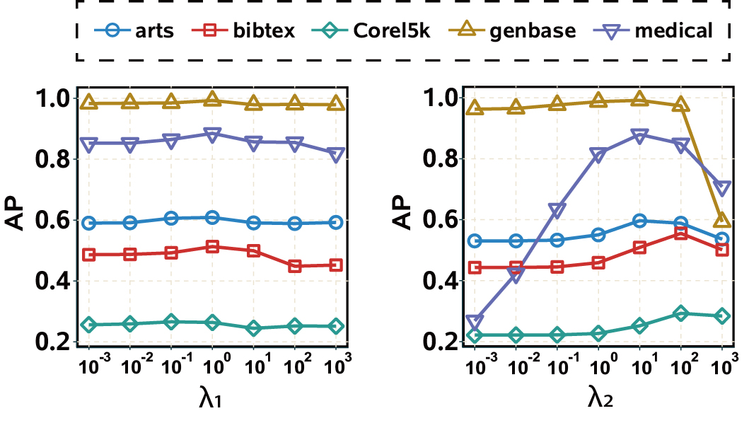
4.3 Parameter Sensitivity

We empirically analyze the sensitivities of the regularization parameters $\{\lambda_{1},\lambda_{2}\}$ of PML³er. For each one, we examine the AP scores by varying its value from $\{10^{i}|i=-3,\cdots,3\}$ across PML datasets with $a=100$ by holding the other two fixed. The experimental results are presented in Fig.2. First, we can observe that the AP scores of $\lambda_{1}$ seem quite stable over different types of PML datasets. That is, we empirically conclude that PML³er is insensitive to $\lambda_{1}$ , making PML³er more practical. Second, for $\lambda_{2}$ , it performs better with the values of $\{10^{i}|i=1,2\}$ across all PML datasets, which are the settings used in our experiment.

5 Conclusion

We concentrate on the task of PML, and propose a novel two-stage PML³er algorithm. In the first stage, PML³er performs an unconstrained label propagation procedure to estimate the label enrichment, which simultaneously involves the relevance degrees of candidate labels and irrelevance degrees of non-candidate labels. In the second stage, PML³er jointly learns the ground-truth confidence and multi-label predictor given the label enrichment. Extensive experiments on PML datasets indicate the superior performance of PML³er.

Acknowledgments

We would like to acknowledge support for this project from the National Natural Science Foundation of China (NSFC) (No.61602204, No.61876071, No.61806035, No.U1936217)

References

Boyd et al. [2011] Stephen Boyd, Neal Parikh, Eric Chu, Borja Peleato, and Jonathan Eckstein. Distributed optimization and statistical learning via the alternating direction method of multipliers. Foundations and Trends in Machine Learning, 3(1):1–122, 2011.
Cai et al. [2010] Jian-Feng Cai, Emmanuel J. Candès, and Zuowei Shen. A singular value thresholding algorithm for matrix completion. SIAM Journal on Optimization, 20(4):1956–1982, 2010.
Chen et al. [2014] Yi-Chen Chen, Vishal M. Patel, Rama Chellappa, and P. Jonathon Phillips. Ambiguously labeled learning using dictionaries. IEEE Transactions on Information Forensics and Security, 9(12):2076–2088, 2014.
Chen et al. [2018] Ching-Hui Chen, Vishal M. Patel, and Rama Chellappa. Learning from ambiguously labeled face images. IEEE Transactions on Pattern Analysis and Machine Intelligence, 40(7):1653–1667, 2018.
Cour et al. [2011] Timothee Cour, Benjamin Sapp, and Ben Taskar. Learning from partial labels. Journal of Machine Learning Research, 12:1501–1536, 2011.
Fang and Zhang [2019] Jun-Peng Fang and Min-Ling Zhang. Partial multi-label learning via credible label elicitation. In AAAI Conference on Artificial Intelligence, pages 3518–3525, 2019.
Feng and An [2018] Lei Feng and Bo An. Leveraging latent label distributions for partial label learning. In International Joint Conference on Artificial Intelligence, pages 2107–2113, 2018.
Feng and An [2019a] Lei Feng and Bo An. Partial label learning by semantic difference maximization. In International Joint Conference on Artificial Intelligence, pages 2294–2300, 2019.
Feng and An [2019b] Lei Feng and Bo An. Partial label learning with self-guided retraining. In AAAI Conference on Artificial Intelligence, pages 3542–3549, 2019.
Gayar et al. [2006] Neamat El Gayar, Friedhelm Schwenker, and Günther Palm. A study of the robustness of kNN classifiers trained using soft labels. In International Conference on Artificial Neural Network in Pattern Recognition, pages 67–80, 2006.
Gong et al. [2018] Chen Gong, Tongliang Liu, Yuanyan Tang, Jian Yang, Jie Yang, and Dacheng Tao. A regularization approach for instance-based superset label learning. IEEE Transactions on Cybernetics, 48(3):967–978, 2018.
Hou et al. [2016] Peng Hou, Xin Geng, and Min-Ling Zhang. Multi-label manifold learning. In AAAI Conference on Artificial Intelligence, pages 1680–1686, 2016.
Jiang et al. [2006] Xiufeng Jiang, Zhang Yi, and Jian Cheng Lv. Fuzzy SVM with a new fuzzy membership function. Neural Computing & Applications, 15(3-4):268–276, 2006.
Li et al. [2015] Yu-Kun Li, Min-Ling Zhang, and Xin Geng. Leveraging implicit relative labeling-importance information for effective multi-label learning. In IEEE International Conference on Data Mining, pages 251–260, 2015.
Liu and Dietterich [2012] Li-Ping Liu and Thomas G. Dietterich. A conditional multinomial mixture model for superset label learning. In Neural Information Processing Systems, pages 548–556, 2012.
Sun et al. [2019] Lijuan Sun, Songhe Feng, Tao Wang, Congyan Lang, and Yi Jin. Partial multi-label learning with low-rank and sparse decomposition. In AAAI Conference on Artificial Intelligence, pages 5016–5023, 2019.
Wang et al. [2019] Deng-Bao Wang, Li Li, and Min-Ling Zhang. Adaptive graph guided disambiguation for partial label learning. In ACM SIGKDD Conference on Knowledge Discovery and Data Mining, pages 83–91, 2019.
Wu and Zhang [2018] Xuan Wu and Min-Ling Zhang. Towards enabling binary decomposition for partial label learning. In International Joint Conference on Artificial Intelligence, pages 2868–2874, 2018.
Xie and Huang [2018] Ming-Kun Xie and Sheng-Jun Huang. Partial multi-label learning. In AAAI Conference on Artificial Intelligence, pages 4302–4309, 2018.
Xu et al. [2018] Ning Xu, An Tao, and Xin Geng. Label enhancement for label distribution learning. In International Joint Conference on Artificial Intelligence, pages 2926–2932, 2018.
Yu and Zhang [2017] Fei Yu and Min-Ling Zhang. Maximum margin partial label learning. Machine Learning, 106:573–593, 2017.
Yu et al. [2018] Guoxian Yu, Xia Chen, Carlotta Domeniconi, Jun Wang, Zhao Li, Zili Zhang, and Xindong Wu. Feature-induced partial multi-label learning. In IEEE International Conference on Data Mining, pages 1398–1403, 2018.
Zhang and Wu [2015] Min-Ling Zhang and Lei Wu. Lift: Multi-label learning with label-specific features. IEEE Transactions on Pattern Analysis and Machine Intelligence, 37(1):107–120, 2015.
Zhang and Zhou [2007] Min-Ling Zhang and Zhi-Hua Zhou. ML-kNN: A lazy learning approach to multi-label learning. Pattern Recognition, 40(7):2038–2048, 2007.
Zhang and Zhou [2014] Min-Ling Zhang and Zhi-Hua Zhou. A review on multi-label learning algorithms. IEEE Transactions on Knowledge and Data Engineering, 26(8):1819–1837, 2014.
Zhang et al. [2017] Min-Ling Zhang, Fei Yu, and Cai-Zhi Tang. Disambiguation-free partial label learning. IEEE Transactions on Knowledge and Data Engineering, 29(10):2155–2167, 2017.