Chirag Nagpal \Emailchiragn@cs.cmu.edu
\NameVedant Sanil \Emailvsanil@andrew.cmu.edu
\NameArtur Dubrawski \Emailawd@cs.cmu.edu
\addrAuton Lab, Carnegie Mellon
Recovering Sparse and Interpretable Subgroups with Heterogeneous Treatment Effects with Censored Time-to-Event Outcomes
Abstract
Studies involving both randomized experiments as well as observational data typically involve time-to-event outcomes such as time-to-failure, death or onset of an adverse condition. Such outcomes are typically subject to censoring due to loss of follow-up and established statistical practice involves comparing treatment efficacy in terms of hazard ratios between the treated and control groups. In this paper we propose a statistical approach to recovering sparse phenogroups (or subtypes) that demonstrate differential treatment effects as compared to the study population. Our approach involves modelling the data as a mixture while enforcing parameter shrinkage through structured sparsity regularization. We propose a novel inference procedure for the proposed model and demonstrate its efficacy in recovering sparse phenotypes across large landmark real world clinical studies in cardiovascular health.
keywords:
Time-to-Event, Survival Analysis, Heterogeneous Treatment Effects, Hazard Ratio1 Introduction
Data driven decision making across multiple disciplines including healthcare, epidemiology, econometrics and prognostics often involves establishing efficacy of an intervention when outcomes are measured in terms of the time to an adverse event, such as death, failure or onset of a critical condition. Typically the analysis of such studies involves assigning a patient population to two or more different treatment arms often called the ‘treated’ (or ‘exposed’) group and the ‘control’ (or ‘placebo’) group and observing whether the populations experience an adverse event (for instance death or onset of a disease) over the study period at a rate that is higher (or lower) than for the control group. Efficacy of a treatment is thus established by comparing the relative difference in the rate of event incidence between the two arms called the hazard ratio. However, not all individuals benefit equally from an intervention. Thus, very often potentially beneficial interventions are discarded even though there might exist individuals who benefit, as the population level estimates of treatment efficacy are inconclusive.
In this paper we assume that patient responses to an intervention are typically heterogeneous and there exists patient subgroups that are unaffected by (or worse, harmed) by the intervention being assessed. The ability to discover or phenotype these patients is thus clinically useful as it would allow for more precise clinical decision making by identifying individuals that actually benefit from the intervention being assessed.
Towards this end, we propose Sparse Cox Subgrouping, (SCS) a latent variable approach to model patient subgroups that demonstrate heterogeneous effects to an intervention. As opposed to existing literature in modelling heterogeneous treatment effects with censored time-to-event outcomes our approach involves structured regularization of the covariates that assign individuals to subgroups leading to parsimonious models resulting in phenogroups that are interpretable. We release a python implementation of the proposed SCS approach as part of the auton-survival package (Nagpal et al., 2022b) for survival analysis:
2 Related Work
Large studies especially in clinical medicine and epidemiology involve outcomes that are time-to-events such as death, or an adverse clinical condition like stroke or cancer. Treatment efficacy is typically estimated by comparing event rates between the treated and control arms using the Proportional Hazards (Cox, 1972) model and its extensions.
Identification of subgroups in such scenarios has been the subject of a large amount of traditional statistical literature. Large number of such approaches involve estimation of the factual and counterfactual outcomes using separate regression models (T-learner) followed by regressing the difference between these estimated potential outcomes. Within this category of approaches, Lipkovich et al. (2011) propose the subgroup identification based on differential effect search (SIDES) algorithm, Su et al. (2009) propose a recursive partitioning method for subgroup discovery, Dusseldorp and Mechelen (2014) propose the qualitative interaction trees (QUINT) algorithm, and Foster et al. (2011) propose the virtual twins (VT) method for subgroup discovery involving decision tree ensembles. We include a parametric version of such an approach as a competing baseline.
Identification of heterogeneous treatment effects (HTE) is also of growing interest to the machine learning community with multiple approaches involving deep neural networks with balanced representations (Shalit et al., 2017; Johansson et al., 2020), generative models Louizos et al. (2017) as well as Non-Parametric methods involving random-forests (Wager and Athey, 2018) and Gaussian Processes (Alaa and Van Der Schaar, 2017). There is a growing interest in estimating HTEs from an interpretable and trustworthy standpoint (Lee et al., 2020; Nagpal et al., 2020; Morucci et al., 2020; Wu et al., 2022; Crabbé et al., 2022). Wang and Rudin (2022) propose a sampling based approach to discovering interpretable rule sets demonstrating HTEs.
However large part of this work has focused extensively on outcomes that are binary or continuous. The estimation of HTEs in the presence of censored time-to-events has been limited. Xu et al. (2022) explore the problem and describe standard approaches to estimate treatment effect heterogeneity with survival outcomes. They also describe challenges associated with existing risk models when assessing treatment effect heterogeneity in the case of cardiovascular health.
There has been some initial attempt to use neural network for causal inference with censored time-to-event outcomes. Curth et al. (2021) propose a discrete time method along with regularization to match the treated and control representations. Chapfuwa et al. (2021)’s approach is related and involves the use of normalizing flows to estimate the potential time-to-event distributions under treatment and control. While our contributions are similar to Nagpal et al. (2022a), in that we assume treatment effect heterogeneity through a latent variable model, our contribution differs in that 1) Our approach is free of the expensive Monte-Carlo sampling procedure and 2) Our generalized EM inference procedure allows us to naturally incorporate structured sparsity regularization, which helps recovers phenogroups that are parsimonious in the features they recover that define subgroups.
Survival and time-to-event outcomes occur pre-eminently in areas of cardiovascular health. One such area is reducing combined risk of adverse outcomes from atherosclerotic disease111A class of related clinical conditions from increasing deposits of plaque in the arteries, leading to Stroke, Myorcardial Infarction and other Coronary Heart Diseases. (Herrington et al., 2016; Furberg et al., 2002; Group, 2009; Buse et al., 2007) The ability of recovering groups with differential benefits to interventions can thus lead to improved patient care through framing of optimal clinical guidelines.
3 Proposed Model: Sparse Cox Subgrouping
Case 1:
Case 2:
- Notation
-
As is standard in survival analysis, we assume that we either observe the true time-to-event or the time of censoring indicated by the censoring indicator defined as . We thus work with a dataset of right censored observations in the form of 4-tuples, , where is the time-to-event or censoring as indicated by , is the indicator of treatment assignment, and are individual covariates that confound the treatment assignment and the outcome.
Assumption 1 (Independent Censoring)
The time-to-event and the censoring distribution are independent conditional on the covariates and the intervention .
- Model
-
Consider a maximum likelihood approach to model the data the set of parameters . Under Assumption 1 the likelihood of the data can be given as,
(1) here is the hazard and is the survival rate.
Assumption 2 (PH)
The distribution of the time-to-event conditional on the covariates and the treatment assignment obeys proportional hazards.
From Assumption 2 (Proportional Hazards), an individual with covariates under intervention under a Cox model with parameters and treatment effect is given as
(2) Here, is an infinite dimensional parameter known as the base survival rate. In practice in the Cox’s model the base survival rate is a nuisance parameter and is estimated non-parametrically. In order to model the heterogeneity of treatment response. We will now introduce a latent variable that mediates treatment response to the model,
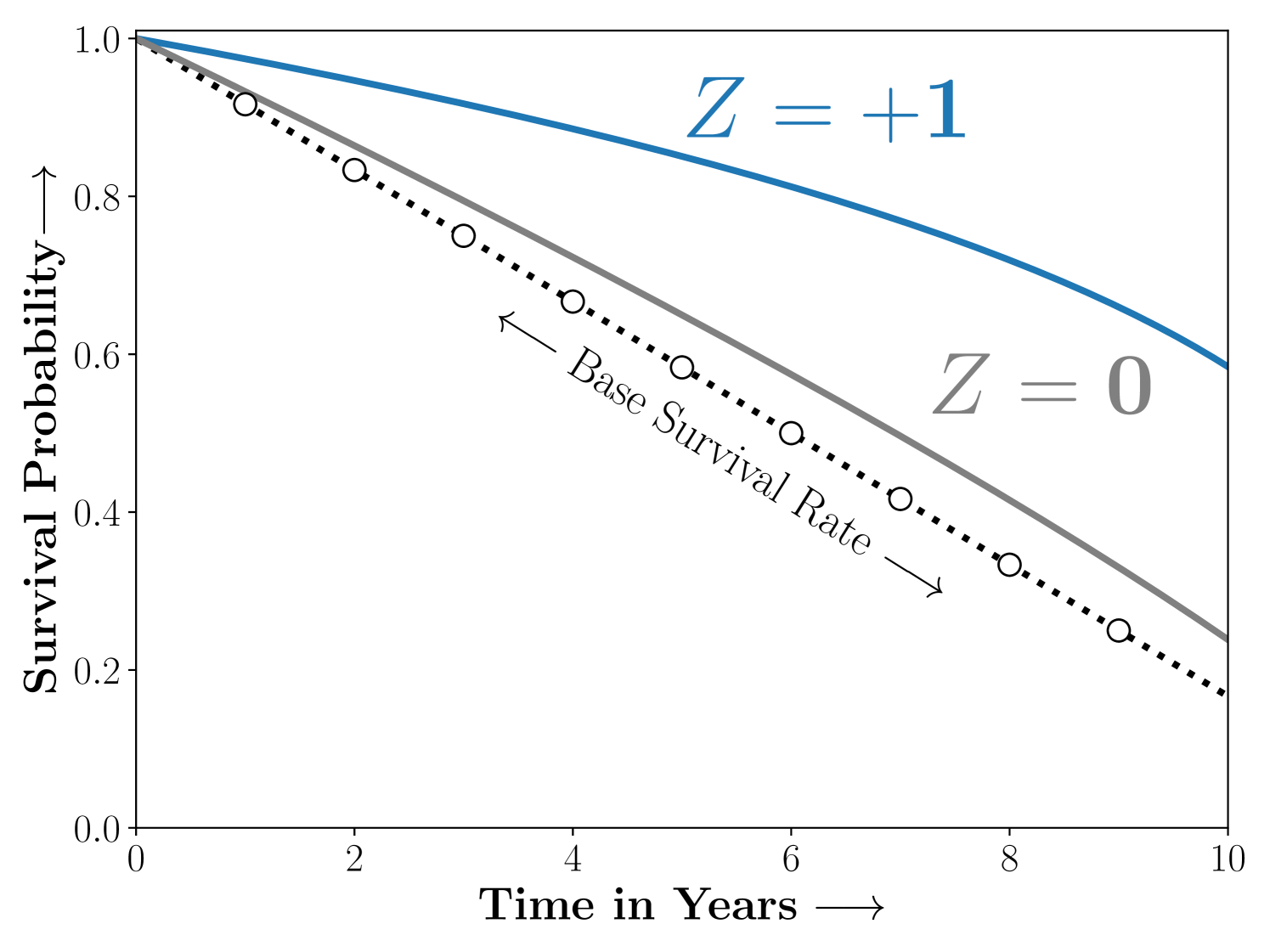
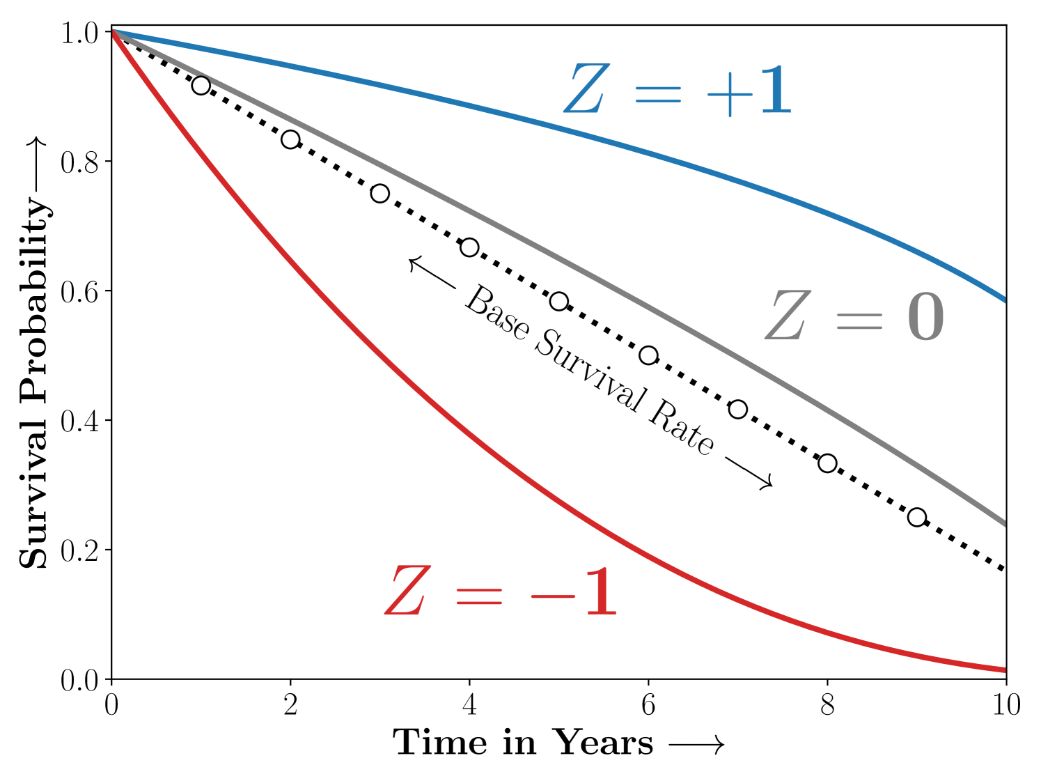
(3) Here, is the treatment effect, and is the set of parameters that mediate assignment to the latent group conditioned on the confounding features . Note that the above choice of parameterization naturally enforces the requirements from the model as in Figure 1. Consider the following scenarios,
Case 1: The study population consists of two sub-strata ie. , that are benefit and are unaffected by treatment respectively.
Case 2: The study population consists of three sub-strata ie. , that benefit, are harmed or unaffected by treatment respectively.
- Shrinkage
-
In retrospective analysis to recover treatment effect heterogeneity a natural requirement is parsimony of the recovered subgroups in terms of the covariates to promote model interpretability. Such parsimony can be naturally enforced through appropriate shrinkage on the coefficients that promote sparsity. We want to recover phenogroups that are ‘sparse’ in . We enforce sparsity in the parameters of the latent gating function via a group (Lasso) penalty. The final loss function to be optimized including the group sparsity regularization term is,
and (5) - Identifiability
-
Further, to ensure identifiability we restrict the gating parameters for the to be . Thus .
- Inference
-
We will present a variation of the Expectation Maximization algorithm to infer the parameters in Equation 3. Our approach differs from Nagpal et al. (2022a, 2021) in that it does not require storchastic Monte-Carlo sampling. Further, our generalized EM inference allows for incorporation of the structured sparsity in the M-Step.
- A Semi-Parametric
-
Note that the likelihood in Equation 3 is semi-parametric and consists of parametric components and the infinite dimensional base hazard . We define the as:
- The E-Step
-
Requires computation of the posteriors counts
Result 1 (Posterior Counts)
The posterior counts for the latent are estimated as,
(6) For a full discussion on derivation of the and the posterior counts please refer to Appendix B
- The M-Step
-
Involves maximizing the function. Rewriting the as a sum of two terms,
Result 2 (Weighted Cox model)
The term can be rewritten as a weighted Cox model and thus optimized using the corresponding ‘partial likelihood’,
Updates for : The partial-likelihood, under sampling weights (Binder, 1992) is
(7) Here is the ‘risk set’ or the set of all individuals who haven’t experienced the event till the corresponding time, i.e. . is convex in and we update these with a gradient step.
Updates for : The base hazard are updated using a weighted Breslow’s estimate (Breslow, 1972; Lin, 2007) assuming the posterior counts to be sampling weights (Chen, 2009),
(8) Term is a function of the gating parameters that determine the latent assignment along with sparsity regularization. We update using a Proximal Gradient update as is the case with Iterative Soft Thresholding (ISTA) for group sparse regression.
Updates for : The proximal update for including the group regularization (Friedman et al., 2010) term is,
(9)
All together the inference procedure is described in Algorithm 1.
[!h]
Parameter Learning for SCS with a Generalized EM
\SetAlgoLined\SetKwInOutInputInput
\SetKwInOutreturnReturn
\InputTraining set, ; maximum EM iterations, , step size
<not converged> \For E-Step .
Compute posterior counts (Equation 6).
M-Step .
Gradient descent update.
Breslow (1972)’s estimator.
Update with gradient of .
Proximal update.
\returnlearnt parameters ;
4 Experiments
In this section we describe the experiments conducted to benchmark the performance of SCS against alternative models for heterogenous treatment effect estimation on multiple studies including a synthetic dataset and multiple large landmark clinical trials for cardiovascular diseases.
4.1 Simulation
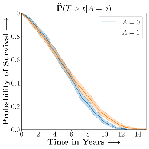
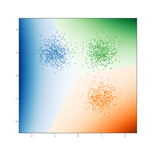
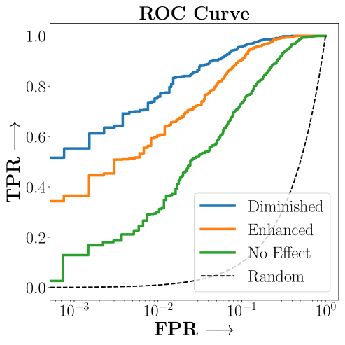
a) The Time-to-Event
b) Learnt Decision Boundary
c) ROC Curves
.
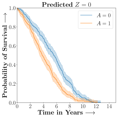
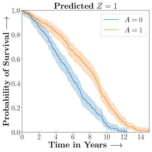
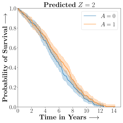
In this section we first describe the performance of the proposed Sparse Cox Subgrouping approach on a synthetic dataset designed to demonstrate heterogeneous treatment effects. We randomly assign individuals to the treated or control group. The latent variable is drawn from a uniform categorical distribution that determines the subgroup,
Conditioned on we sample as in Figure 2 that determine the conditional Hazard Ratios , and randomly sample noisy covariates . The true time-to-event and censoring times are then sampled as,
Finally we sample the censoring indicator and set the observed time-to-event,
Figure 2 presents the ROC curves for SCS’s ability to identify the groups with enhanced and diminished treatment effects respectively. In Figure 3 we present Kaplan-Meier estimators of the Time-to-Event distributions conditioned on the predicted by SCS. Clearly, SCS is able to identify the phenogroups corresponding to differential benefits.
4.2 Recovering subgroups demonstrating Heterogeneous Treatment Effects from Landmark studies of Cardiovascular Health
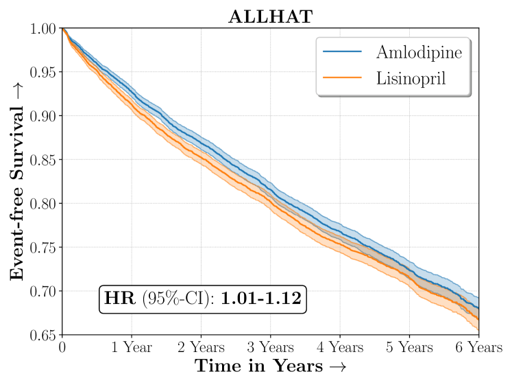
| ALLHAT | |
|---|---|
| Size | 18,102 |
| Outcome | Combined CVD |
| Intervention | Lisinopril |
| Control | Amlodipine |
| Hazard Ratio | 1.06, (1.01, 1.12) |
| 5-year RMST | -24.86, (-37.35, -8.89) |
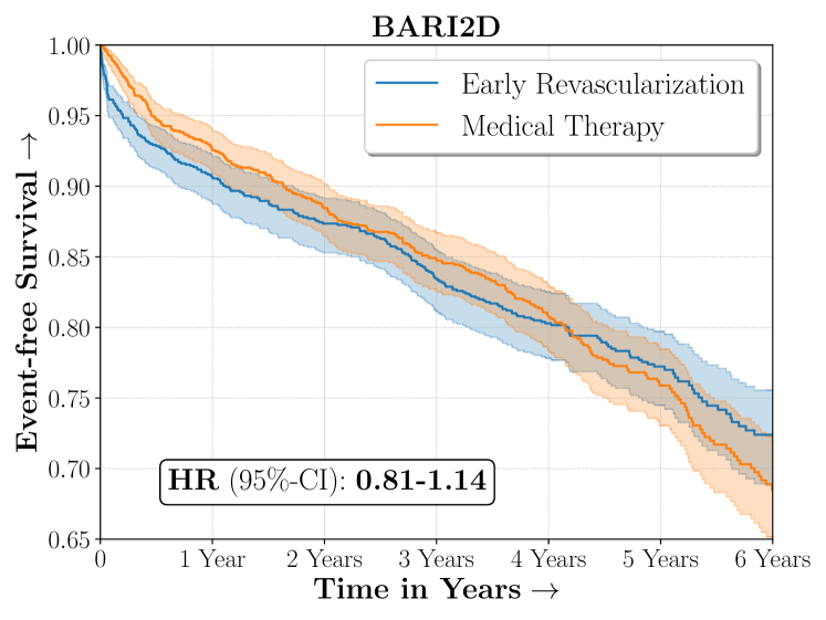
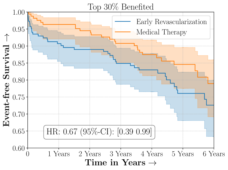
| BARI2D | |
|---|---|
| Size | 2,368 |
| Outcome | Death, MI or Stroke |
| Intervention | Medical Therapy |
| Control | Early Revascularization |
| Hazard Ratio | 1.02, (0.81, 1.14) |
| 5-year RMST | 23.26, (-27.01, 64.84) |
- Antihypertensive and Lipid-Lowering Treatment to Prevent Heart Attack
-
(Furberg et al., 2002)
The ALLHAT study was a large randomized experiment conducted to assess the efficacy of multiple classes of blood pressure lowering medicines for patients with hypertension in reducing risk of adverse cardiovascular conditions. We considered a subset of patients from the original ALLHAT study who were randomized to receive either Amlodipine (a calcium channel blocker) or Lisinopril (an Angiotensin-converting enzyme inhibitor). Overall, Amlodipine was found to be more efficacious than Lisinopril in reducing combined risk of cardio-vascular disease.
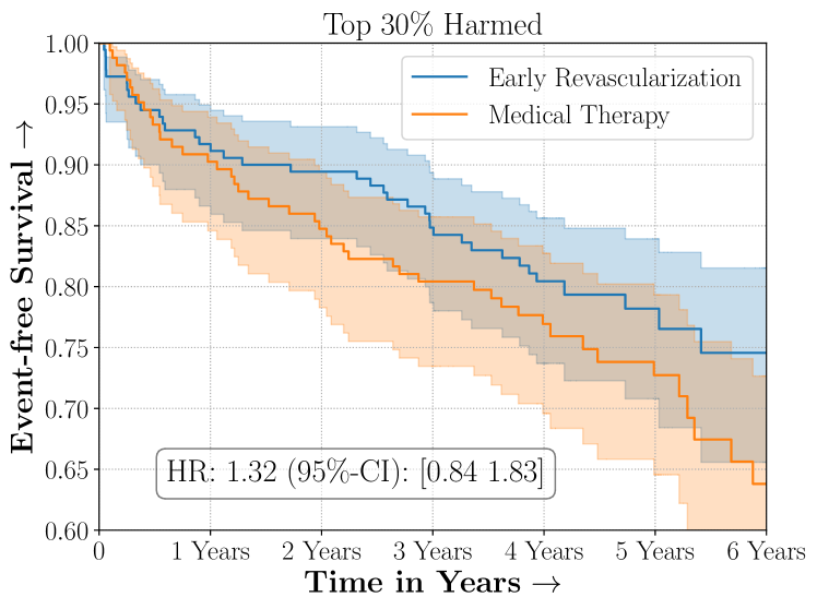
- Bypass Angioplasty Revascularization Investigation in Type II Diabetes
-
(Group, 2009)
Diabetic patients have been traditionally known to be at higher risk of cardiovascular disease however appropriate intervention for diabetics with ischemic heart disease between surgical coronary revascularization or management with medical therapy is widely debated. The BARI2D was a large landmark experiment conducted to assess efficacy between these two possible medical interventions. Overall BARI2D was inconclusive in establishing the appropriate therapy between Coronary Revascularization or medical management for patients with Type-II Diabetes.
Figure 4 presents the event-free survival rates as well as the summary statistics for the studies. In our experiments, we included a large set of confounders collected at baseline visit of the patients which we utilize to train the proposed model. A full list of these features are in Appendix A.
4.3 Baselines
- Cox PH with Regularized Treatment Interaction (cox-int)
-
We include treatment effect heterogeneity via interaction terms that model the time-to-event distribution using a proportional hazards model as in Kehl and Ulm (2006). Thus,
(10) The interaction effects are regularized with a lasso penalty in order to recover a sparse phenotyping rule defined as .
- Binary Classifier with Regularized Treatment Interaction (bin-int)
-
Instead of modelling the time-to-event distribution we directly model the thresholded survival outcomes at a five year time horizon using a log-linear parameterization with a logit link function. As compared to cox-int, this model ignores the data-points that were right-censored prior to the thresholded time-to-event, however it is not sensitive to the strong assumption of Proportional Hazards.
(11) - Cox PH T-Learner with Regularized Logistic Regression (cox-tlr)
-
We train two separate Cox Regression models on the treated and control arms (T-Learner) to estimate the potential outcomes under treatment and control . Motivated from the ‘Virtual Twins’ approach as in Foster et al. (2011), a logistic regression with an penalty is trained to estimate if the risk of the potential outcome under treatment is higher than under control. This logistic regression is then employed as the phenotyping function and is given as,
(12) The above models involving sparse regularization were trained with the glmnet (Friedman et al., 2009) package in R.
- The ACC/AHA Long term Atheroscleoratic Cardiovascular Risk Estimate
-
222https://tools.acc.org/ascvd-risk-estimator-plus/
The American College of Cardiology and the American Heart Association model for estimation of risk of Atheroscleratic disease risk (Goff Jr et al., 2014) involves pooling data from multiple observational cohorts of patients followed by modelling the 10-year risk of an adverse cardiovascular condition including death from coronary heart disease, Non-Fatal Myocardial Infarction or Non-fatal Stroke. While the risk model was originally developed to assess factual risk in the observational sense, in practice it is also employed to assess risk when making counterfactual decisions.
Amlodipine versus Lisinopril in the ALLHAT Study


 No Sparsity

Early Revascularization versus Medical Therapy in the BARI2D Study


 No Sparsity

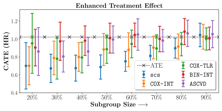
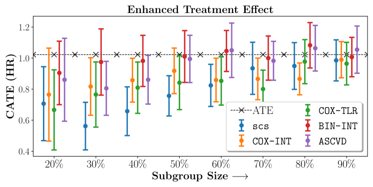
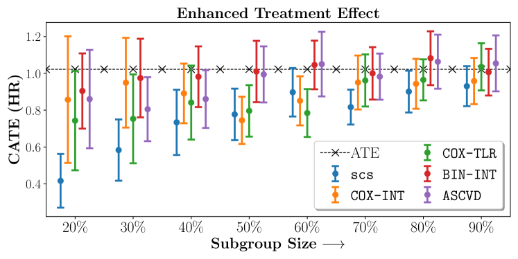
4.4 Results and Discussion
- Protocol
-
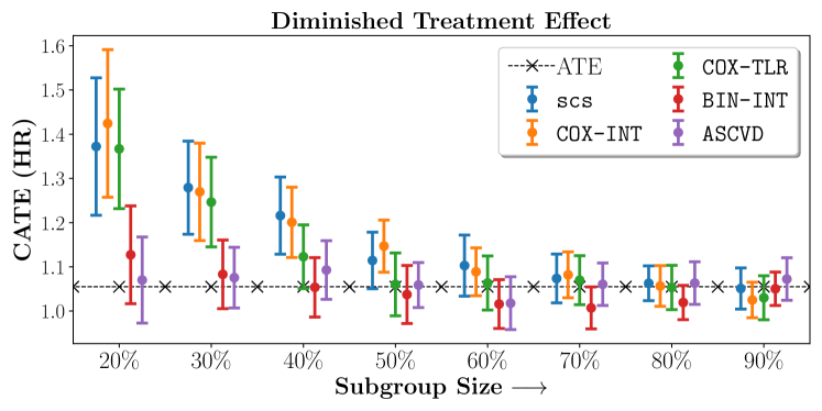
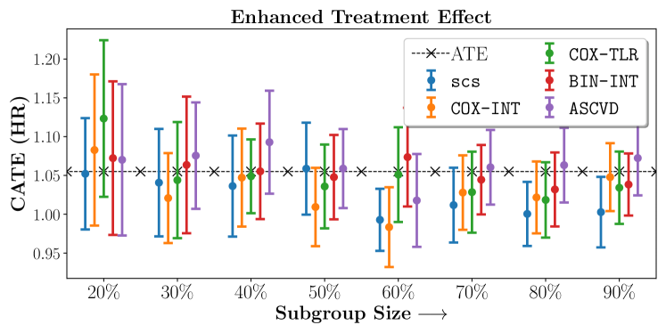
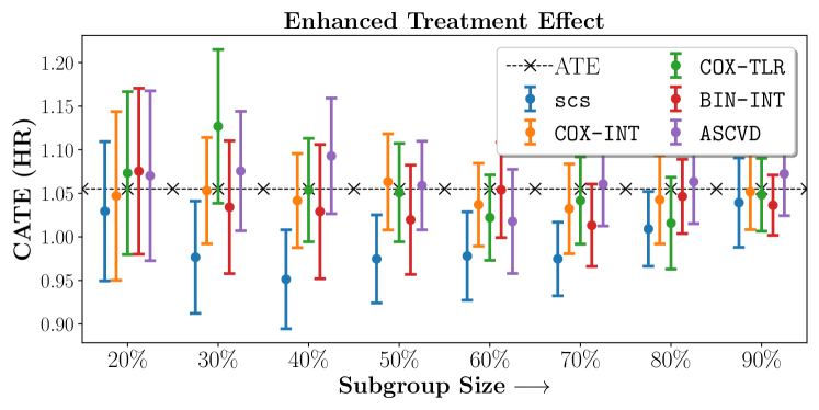
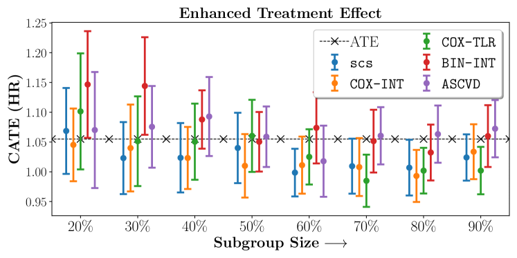
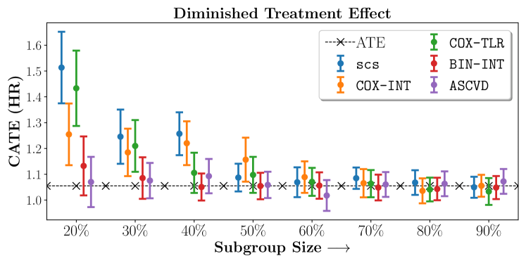
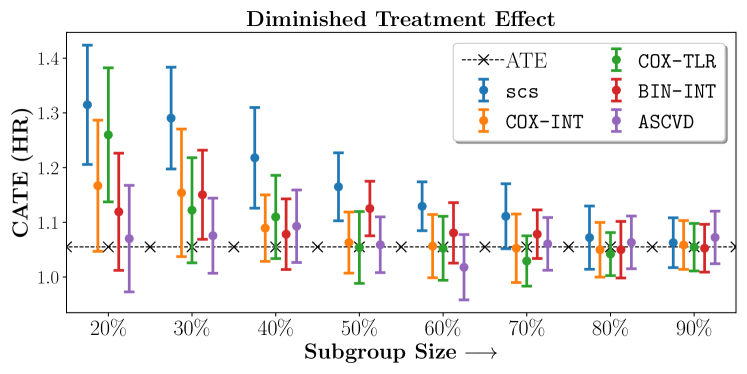
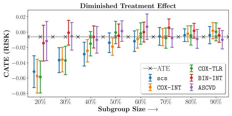
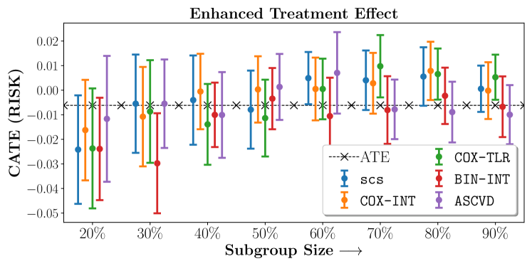
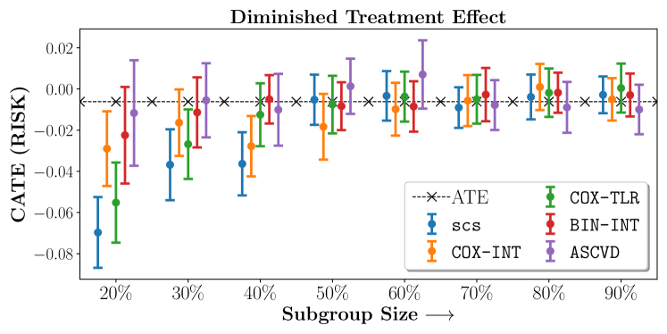
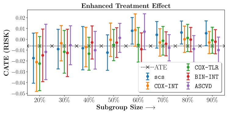
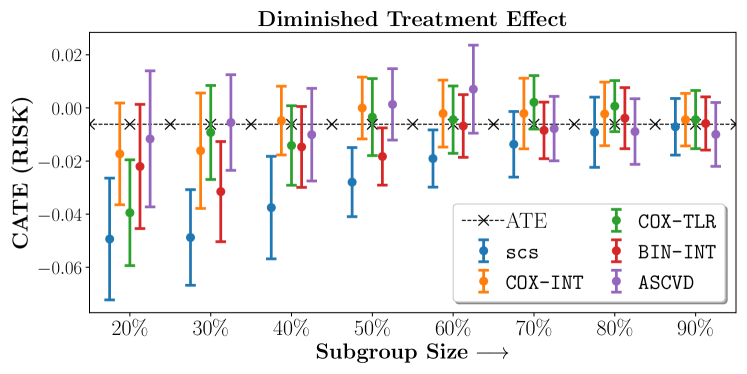
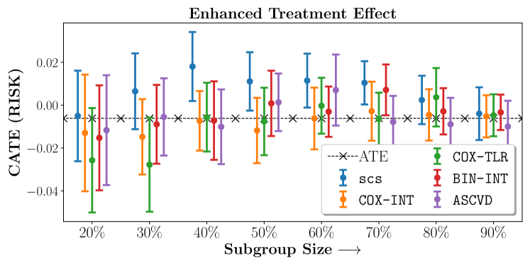
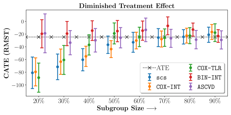
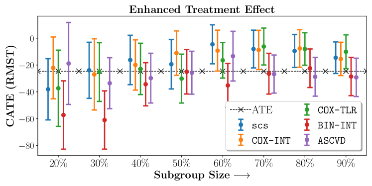
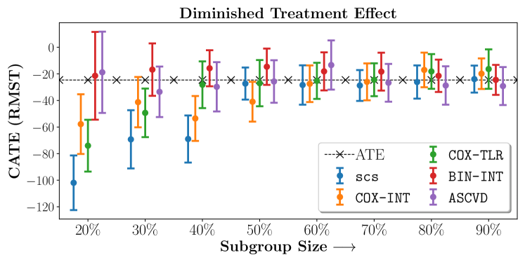
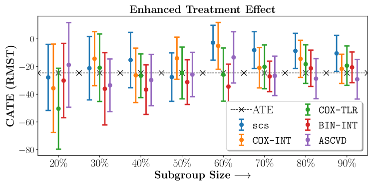
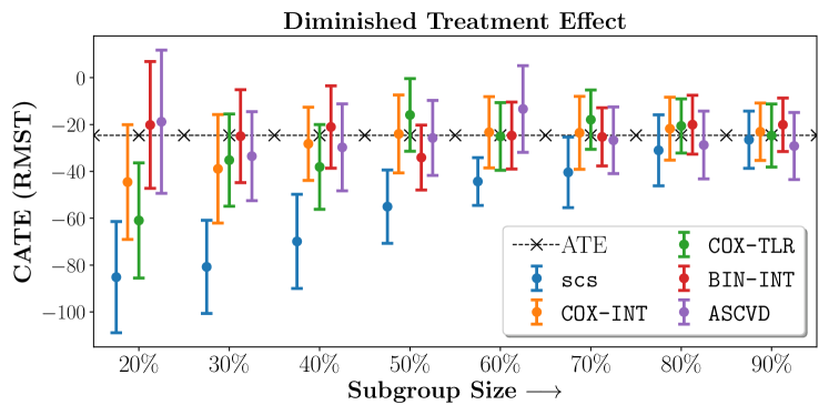
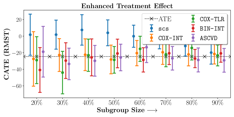
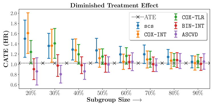
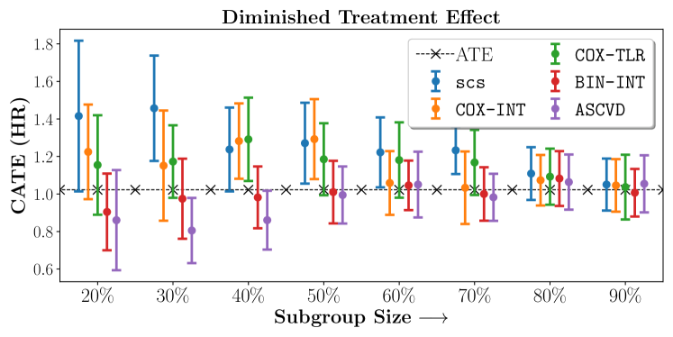
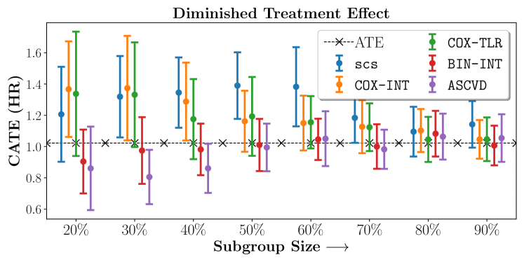
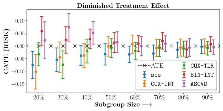
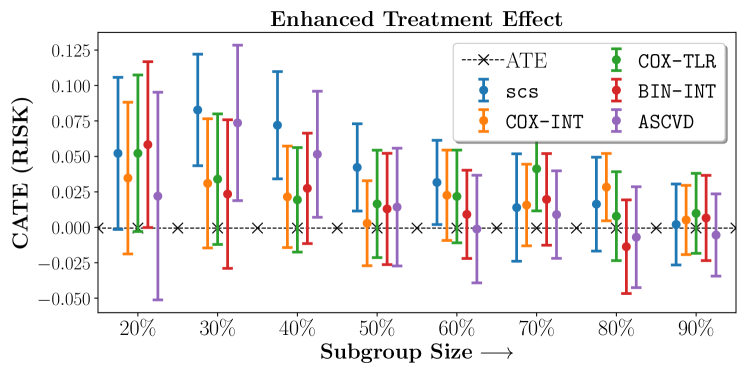
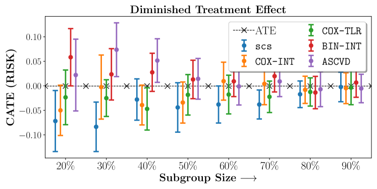
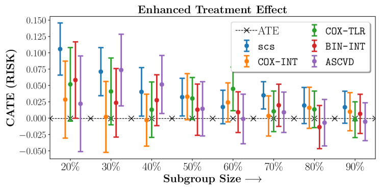
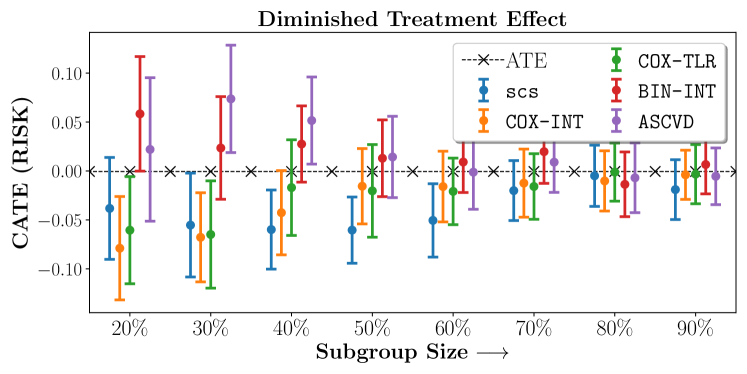
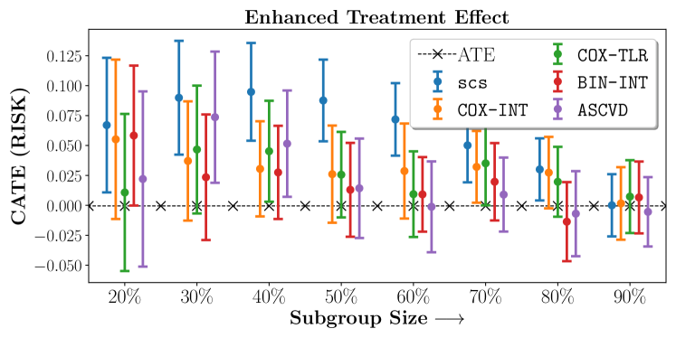
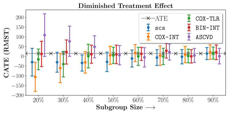
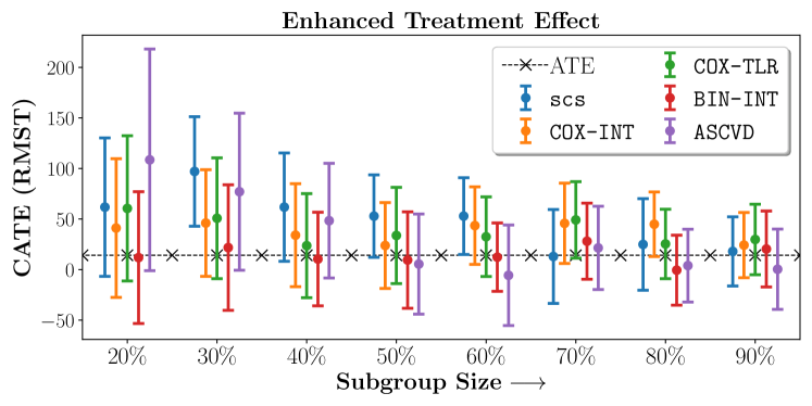
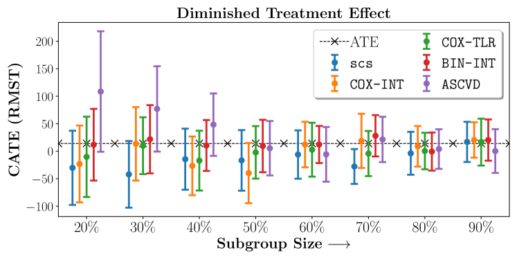
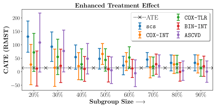
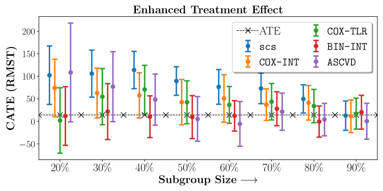
We compare the performance of SCS and the corresponding competing methods in recovery of subgroups with enhanced (or diminished treatment effects). For each of these studies we stratify the study population into equal sized sets for training and validation while persevering the proportion of individuals that were assigned to treatment and experienced the outcome in the follow up period. The models were trained on the training set and validated on the held-out test set. For each of the methods we experiment with models that do not enforce any sparsity () as well as tune the level of sparsity to recover phenotyping functions that involve and features. The subgroup size are varied by controlling the threshold at which the individual is assigned to a group. Finally, the treatment effect is compared in terms of Hazard Ratios, Risk Differences as well as Restricted Mean Survival Time over a 5 Year event period.
- Results
-
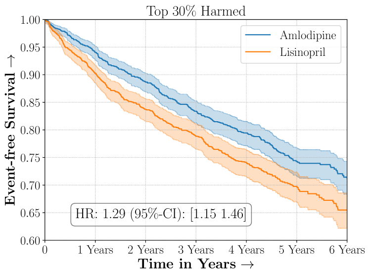
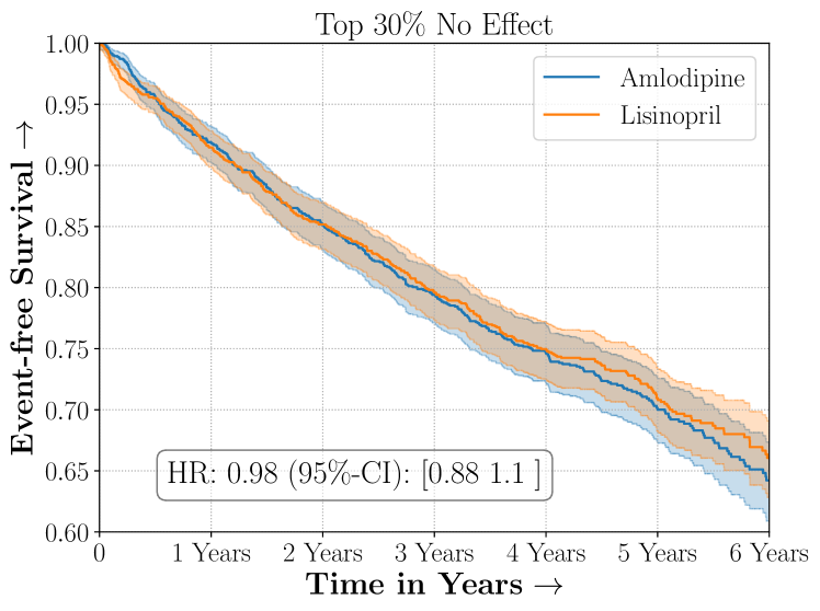
We present the results of SCS versus the baselines in terms of Hazard Ratios on the ALLHAT and BARI2D datasets in Figures 5 and 6. In the case of ALLHAT, SCS consistently recovered phenogroups with more pronounced (or diminished) treatment effects. On external validation on the heldout dataset, we found a subgroup of patients that had similar outcomes whether assigned to Lisinopril or Amlodipine, whereas the other subgroup clearly identified patients that were harmed with Lisinopril. The group harmed with Lisinopril had higher Diastolic BP. On the other hand, patients with Lower kidney function did not seem to benefit from Amlodipine.
In the case of BARI2D, SCS recovered phenogroups that were both harmed as well as benefitted from just medical therapy without revascularization. The patients who were harmed from Medical therapy were typically older, on the other hand the patients who benefitted primarily included patients who were otherwise assigned to receive PCI instead of CABG revascularization, suggesting PCI to be harmful for diabetic patients.
5 Concluding Remarks
We presented Sparse Cox Subgrouping (SCS) a latent variable approach to recover subgroups of patients that respond differentially to an intervention in the presence of censored time-to-event outcomes. As compared to alternative approaches to learning parsimonious hypotheses in such settings, our proposed model recovered hypotheses with more pronounced treatment effects which we validated on multiple studies for cardiovascular health.
While powerful in its ability to recover parsimonious subgroups there exists limitations in SCS in its current form. The model is sensitive to proportional hazards and may be ill-specified when the proportional hazards assumptions are violated as is evident in many real world clinical studies (Maron et al., 2018; Bretthauer et al., 2022). Another limitation is that SCS in its current form looks at only a single endpoint (typically death, or a composite of multiple adverse outcome). In practice however real world studies typically involve multiple end-points. We envision that extensions of SCS would allow patient subgrouping across multiple endpoints, leading to discovery of actionable sub-populations that similarly benefit from the intervention under assessment.
References
- Alaa and Van Der Schaar (2017) Ahmed M Alaa and Mihaela Van Der Schaar. Bayesian inference of individualized treatment effects using multi-task gaussian processes. Advances in neural information processing systems, 30, 2017.
- Binder (1992) David A Binder. Fitting cox’s proportional hazards models from survey data. Biometrika, 79(1):139–147, 1992.
- Breslow (1972) Norman E Breslow. Contribution to discussion of paper by dr cox. J. Roy. Statist. Soc., Ser. B, 34:216–217, 1972.
- Bretthauer et al. (2022) Michael Bretthauer, Magnus Løberg, Paulina Wieszczy, Mette Kalager, Louise Emilsson, Kjetil Garborg, Maciej Rupinski, Evelien Dekker, Manon Spaander, Marek Bugajski, et al. Effect of colonoscopy screening on risks of colorectal cancer and related death. New England Journal of Medicine, 2022.
- Buse et al. (2007) John B Buse, ACCORD Study Group, et al. Action to control cardiovascular risk in diabetes (accord) trial: design and methods. The American journal of cardiology, 99(12):S21–S33, 2007.
- Chapfuwa et al. (2021) Paidamoyo Chapfuwa, Serge Assaad, Shuxi Zeng, Michael J Pencina, Lawrence Carin, and Ricardo Henao. Enabling counterfactual survival analysis with balanced representations. In Proceedings of the Conference on Health, Inference, and Learning, pages 133–145, 2021.
- Chen (2009) Yi-Hau Chen. Weighted breslow-type and maximum likelihood estimation in semiparametric transformation models. Biometrika, 96(3):591–600, 2009.
- Cox (1972) David R Cox. Regression models and life-tables. Journal of the Royal Statistical Society: Series B (Methodological), 34(2):187–202, 1972.
- Crabbé et al. (2022) Jonathan Crabbé, Alicia Curth, Ioana Bica, and Mihaela van der Schaar. Benchmarking heterogeneous treatment effect models through the lens of interpretability. arXiv preprint arXiv:2206.08363, 2022.
- Curth et al. (2021) Alicia Curth, Changhee Lee, and Mihaela van der Schaar. Survite: Learning heterogeneous treatment effects from time-to-event data. Advances in Neural Information Processing Systems, 34:26740–26753, 2021.
- Dusseldorp and Mechelen (2014) Elise Dusseldorp and Iven Mechelen. Qualitative interaction trees: A tool to identify qualitative treatment-subgroup interactions. Statistics in medicine, 33, 01 2014. 10.1002/sim.5933.
- Foster et al. (2011) Jared C Foster, Jeremy MG Taylor, and Stephen J Ruberg. Subgroup identification from randomized clinical trial data. Statistics in medicine, 30(24):2867–2880, 2011.
- Friedman et al. (2009) Jerome Friedman, Trevor Hastie, Rob Tibshirani, et al. glmnet: Lasso and elastic-net regularized generalized linear models. R package version, 1(4):1–24, 2009.
- Friedman et al. (2010) Jerome Friedman, Trevor Hastie, and Robert Tibshirani. A note on the group lasso and a sparse group lasso. arXiv preprint arXiv:1001.0736, 2010.
- Furberg et al. (2002) Curt D Furberg et al. Major outcomes in high-risk hypertensive patients randomized to angiotensin-converting enzyme inhibitor or calcium channel blocker vs diuretic: the antihypertensive and lipid-lowering treatment to prevent heart attack trial (allhat). Journal of the American Medical Association, 2002.
- Goff Jr et al. (2014) David C Goff Jr, Donald M Lloyd-Jones, Glen Bennett, Sean Coady, Ralph B D’agostino, Raymond Gibbons, Philip Greenland, Daniel T Lackland, Daniel Levy, Christopher J O’donnell, et al. 2013 acc/aha guideline on the assessment of cardiovascular risk: a report of the american college of cardiology/american heart association task force on practice guidelines. Circulation, 129(25_suppl_2):S49–S73, 2014.
- Group (2009) BARI 2D Study Group. A randomized trial of therapies for type 2 diabetes and coronary artery disease. New England Journal of Medicine, 360(24):2503–2515, 2009.
- Herrington et al. (2016) William Herrington, Ben Lacey, Paul Sherliker, Jane Armitage, and Sarah Lewington. Epidemiology of atherosclerosis and the potential to reduce the global burden of atherothrombotic disease. Circulation research, 118(4):535–546, 2016.
- Johansson et al. (2020) Fredrik D Johansson, Uri Shalit, Nathan Kallus, and David Sontag. Generalization bounds and representation learning for estimation of potential outcomes and causal effects. arXiv preprint arXiv:2001.07426, 2020.
- Kehl and Ulm (2006) Victoria Kehl and Kurt Ulm. Responder identification in clinical trials with censored data. Computational Statistics & Data Analysis, 50(5):1338–1355, 2006.
- Lee et al. (2020) Kwonsang Lee, Falco J Bargagli-Stoffi, and Francesca Dominici. Causal rule ensemble: Interpretable inference of heterogeneous treatment effects. arXiv preprint arXiv:2009.09036, 2020.
- Lin (2007) DY Lin. On the breslow estimator. Lifetime data analysis, 13(4):471–480, 2007.
- Lipkovich et al. (2011) Ilya Lipkovich, Alex Dmitrienko, Jonathan Denne, and Gregory Enas. Subgroup identification based on differential effect search (sides) – a recursive partitioning method for establishing response to treatment in patient subpopulations. Statistics in medicine, 30:2601–21, 07 2011. 10.1002/sim.4289.
- Louizos et al. (2017) Christos Louizos, Uri Shalit, Joris M Mooij, David Sontag, Richard Zemel, and Max Welling. Causal effect inference with deep latent-variable models. Advances in neural information processing systems, 30, 2017.
- Maron et al. (2018) David J Maron, Judith S Hochman, Sean M O’Brien, Harmony R Reynolds, William E Boden, Gregg W Stone, Sripal Bangalore, John A Spertus, Daniel B Mark, Karen P Alexander, et al. International study of comparative health effectiveness with medical and invasive approaches (ischemia) trial: rationale and design. American heart journal, 201:124–135, 2018.
- Morucci et al. (2020) Marco Morucci, Vittorio Orlandi, Sudeepa Roy, Cynthia Rudin, and Alexander Volfovsky. Adaptive hyper-box matching for interpretable individualized treatment effect estimation. In Conference on Uncertainty in Artificial Intelligence, pages 1089–1098. PMLR, 2020.
- Nagpal et al. (2020) Chirag Nagpal, Dennis Wei, Bhanukiran Vinzamuri, Monica Shekhar, Sara E Berger, Subhro Das, and Kush R Varshney. Interpretable subgroup discovery in treatment effect estimation with application to opioid prescribing guidelines. In Proceedings of the ACM Conference on Health, Inference, and Learning, pages 19–29, 2020.
- Nagpal et al. (2021) Chirag Nagpal, Steve Yadlowsky, Negar Rostamzadeh, and Katherine Heller. Deep cox mixtures for survival regression. In Machine Learning for Healthcare Conference, pages 674–708. PMLR, 2021.
- Nagpal et al. (2022a) Chirag Nagpal, Mononito Goswami, Keith Dufendach, and Artur Dubrawski. Counterfactual phenotyping with censored time-to-events. In Proceedings of the 28th ACM SIGKDD Conference on Knowledge Discovery and Data Mining, KDD ’22, page 3634–3644, New York, NY, USA, 2022a. Association for Computing Machinery. ISBN 9781450393850. 10.1145/3534678.3539110. URL https://doi.org/10.1145/3534678.3539110.
- Nagpal et al. (2022b) Chirag Nagpal, Willa Potosnak, and Artur Dubrawski. auton-survival: an open-source package for regression, counterfactual estimation, evaluation and phenotyping with censored time-to-event data. In Proceedings of the 7th Machine Learning for Healthcare Conference, volume 182 of Proceedings of Machine Learning Research, pages 585–608. PMLR, 05–06 Aug 2022b. URL https://proceedings.mlr.press/v182/nagpal22a.html.
- Shalit et al. (2017) Uri Shalit, Fredrik D Johansson, and David Sontag. Estimating individual treatment effect: generalization bounds and algorithms. In International Conference on Machine Learning, pages 3076–3085. PMLR, 2017.
- Su et al. (2009) Xiaogang Su, Chih-Ling Tsai, Hansheng Wang, David Nickerson, and Bogong Li. Subgroup analysis via recursive partitioning. Journal of Machine Learning Research, 10:141–158, 02 2009. 10.2139/ssrn.1341380.
- Wager and Athey (2018) Stefan Wager and Susan Athey. Estimation and inference of heterogeneous treatment effects using random forests. Journal of the American Statistical Association, 113(523):1228–1242, 2018.
- Wang and Rudin (2022) Tong Wang and Cynthia Rudin. Causal rule sets for identifying subgroups with enhanced treatment effects. INFORMS Journal on Computing, 2022.
- Wu et al. (2022) Han Wu, Sarah Tan, Weiwei Li, Mia Garrard, Adam Obeng, Drew Dimmery, Shaun Singh, Hanson Wang, Daniel Jiang, and Eytan Bakshy. Interpretable personalized experimentation. In Proceedings of the 28th ACM SIGKDD Conference on Knowledge Discovery and Data Mining, pages 4173–4183, 2022.
- Xu et al. (2022) Yizhe Xu, Nikolaos Ignatiadis, Erik Sverdrup, Scott Fleming, Stefan Wager, and Nigam Shah. Treatment heterogeneity with survival outcomes. arXiv preprint arXiv:2207.07758, 2022.
Appendix A Additional Details on the ALLHAT and BARI 2D Case Studies
Tables 1 and 2 represent additional confounding variables found in the ALLHAT and BARI2D trials respectively.
| Name | Description |
|---|---|
| ETHNIC | Ethnicity |
| SEX | Sex of Participant |
| ESTROGEN | Estrogen supplementation |
| BLMEDS | Antihypertensive treatment |
| MISTROKE | History of Stroke |
| HXCABG | History of coronary artery bypass |
| STDEPR | Prior ST depression/T-wave inversion |
| OASCVD | Other atherosclerotic cardiovascular disease |
| DIABETES | Prior history of Diabetes |
| HDLLT35 | HDL cholesterol <35mg/dl; 2x in past 5 years |
| LVHECG | LVH by ECG in past 2 years |
| WALL25 | LVH by ECG in past 2 years |
| LCHD | History of CHD at baseline |
| CURSMOKE | Current smoking status. |
| ASPIRIN | Aspirin use |
| LLT | Lipid-lowering trial |
| AGE | Age upon entry |
| BLWGT | Weight upon entry |
| BLHGT | Height upon entry |
| BLBMI | Body Mass Index upon entry |
| BV2SBP | Baseline SBP |
| BV2DBP | Baseline DBP |
| APOTAS | Baseline serum potassium |
| BLGFR | Baseline est glomerular filtration rate |
| ACHOL | Total Cholesterol |
| AHDL | Baseline HDL Cholesterol |
| AFGLUC | Baseline fasting serum glucose |
| Name | Description |
|---|---|
| hxmi | History of MI |
| age | Age upon entry |
| dbp_stand | Standing diastolic BP |
| sbp_stand | Standing systolic BP |
| sex | Sex |
| asp | Aspirin use |
| smkcat | Cigarette smoking category |
| betab | Beta blocker use |
| ccb | Calcium blocker use |
| hxhtn | History of hypertension requiring tx |
| insulin | Insulin use |
| weight | Weight (kg) upon entry |
| bmi | BMI upon entry |
| qabn | Abnormal Q-Wave |
| trig | Triglycerides (mg/dl) upon entry |
| dmdur | Duration of diabetes mellitus |
| ablvef | Left ventricular ejection fraction <50% |
| race | Race |
| priorrev | Prior revascularization |
| hxcva | Cerebrovascular accident |
| screat | Serum creatinine (mg/dl) |
| hmg | Statin |
| hxhypo | History of hypoglycemic episode |
| hba1c | Hemoglobin A1c(%) |
| priorstent | Prior stent |
| spotass | Serum Potassium(mEq/L) |
| hispanic | Hispanic ethnicity |
| tchol | Total Cholesterol |
| hdl | HDL Cholesterol |
| insul_circ | Circulating insulin (IU/ml) |
| tzd | Thiazolidinedione |
| ldl | LDL Cholesterol |
| tabn | Abnormal T-waves |
| nsgn | Nonsublingual nitrate |
| sulf | Sulfonylurea |
| hxchf | Histoty of congestive heart failure req tx |
| arb | Angiotensin receptor blocker |
| acr | Urine albumin/creatinine ratio mg/g |
| diur | Diuretic |
| apa | Anti-platelet |
| hxchl | Hypercholesterolemia req tx |
| acei | ACE inhibitor |
| abilow | Low ABI (<= 0.9) |
| biguanide | Biguanide |
| stabn | Abnormal ST depression |
ALLHAT Name Description BV2SBP Baseline Seated Diastolic Pressure BLGFR Baseline est Glomerular Filteration Rate BLMEDS Antihypertensive Treatment CURSMOKE Current Smoking Status SEX Sex of Participant
BARI2D Name Description age Age upon entry asp Aspirin use hxhtn History of hypertension requiring tx hxchl Hypercholesterolemia req tx priorstent Prior stent
ALLHAT Name Description BV2SBP Baseline Seated Diastolic Pressure BLGFR Baseline est Glomerular Filtration Rate BLMEDS Antihypertensive Treatment CURSMOKE Current Smoking Status SEX Sex of Participant ASPIRIN Aspirin Use ACHOL Total Cholesterol BLWGT Weight upon entry BMI Body mass index upon entry OASCVD Other atherosclerotic cardiovascular disease
BARI2D Name Description age Age upon entry asp Aspirin use hxhtn History of hypertension requiring tx hxchl Hypercholesterolemia req tx priorstent Prior stent acei ACE Inhibitor acr Urine albumin/creatinine ratio mg/g insul_circ Circulating insulin screat Serum creatinine (mg/dl) tchol Total Cholesterol
Appendix B Derivation of the Inference Algorithm
Censored Instances: Note that in the case of the censored instances we will condition on the thresholded survival . The the posterior counts thus reduce to:
| (13) |
Uncensored Instances The posteriors are ,
Posteriors for the uncensored data are more involved and involve the base hazard . Posteriors for uncensored data are independent of the base hazard function, as,
| (14) |
Appendix C Additional Results
Figures 7, 8, 9 present tabulated metrics on ALLHAT with Hazard Ratio, Risk Difference and Restricted Mean Survival Time respectively. Figures 10, 11, 12 present tabulated metrics BARI2D with Hazard Ratio, Risk Difference and Restricted Mean Survival Time metrics respectively.

20%
40%
60%
80%
SCS
1.310.11
1.220.09
1.130.04
1.070.06
COX-INT
1.170.12
1.090.06
1.060.06
1.050.05
COX-TLR
1.260.12
1.110.08
1.050.06
1.040.04
BIN-INT
1.120.11
1.080.06
1.080.06
1.050.05
ASCVD
1.070.1
1.090.07
1.020.06
1.060.05
20%
40%
60%
80%
SCS
1.030.08
0.950.06
0.980.05
1.010.04
COX-INT
1.050.1
1.040.05
1.040.05
1.040.05
COX-TLR
1.070.09
1.050.06
1.020.05
1.020.05
BIN-INT
1.080.1
1.030.08
1.050.05
1.050.04
ASCVD
1.070.1
1.090.07
1.020.06
1.060.05

| 20% | 40% | 60% | 80% | |
|---|---|---|---|---|
| SCS | 1.510.14 | 1.260.08 | 1.070.06 | 1.070.05 |
| COX-INT | 1.250.12 | 1.220.08 | 1.090.06 | 1.040.05 |
| COX-TLR | 1.430.15 | 1.110.08 | 1.070.05 | 1.040.05 |
| BIN-INT | 1.130.11 | 1.050.05 | 1.060.05 | 1.040.04 |
| ASCVD | 1.070.1 | 1.090.07 | 1.020.06 | 1.060.05 |
| 20% | 40% | 60% | 80% | |
|---|---|---|---|---|
| SCS | 1.050.07 | 1.040.07 | 0.990.04 | 1.00.04 |
| COX-INT | 1.080.1 | 1.050.06 | 0.980.05 | 1.020.05 |
| COX-TLR | 1.120.1 | 1.050.05 | 1.050.06 | 1.020.05 |
| BIN-INT | 1.070.1 | 1.060.06 | 1.070.06 | 1.030.05 |
| ASCVD | 1.070.1 | 1.090.07 | 1.020.06 | 1.060.05 |
No Sparsity

| 20% | 40% | 60% | 80% | |
|---|---|---|---|---|
| SCS | 1.370.16 | 1.220.09 | 1.10.07 | 1.060.04 |
| COX-INT | 1.420.17 | 1.20.08 | 1.090.05 | 1.060.05 |
| COX-TLR | 1.370.14 | 1.120.07 | 1.060.06 | 1.050.05 |
| BIN-INT | 1.130.11 | 1.050.07 | 1.020.06 | 1.020.04 |
| ASCVD | 1.070.1 | 1.090.07 | 1.020.06 | 1.060.05 |
| 20% | 40% | 60% | 80% | |
|---|---|---|---|---|
| SCS | 1.070.07 | 1.020.06 | 1.00.04 | 1.010.05 |
| COX-INT | 1.050.06 | 1.020.05 | 1.010.05 | 0.990.04 |
| COX-TLR | 1.10.1 | 1.050.06 | 1.030.05 | 1.00.04 |
| BIN-INT | 1.150.09 | 1.090.05 | 1.070.06 | 1.030.05 |
| ASCVD | 1.070.1 | 1.090.07 | 1.020.06 | 1.060.05 |
 20%
40%
60%
80%
SCS
-0.050.02
-0.030.02
-0.010.01
-0.00.01
COX-INT
-0.060.02
-0.020.01
-0.010.01
-0.00.01
COX-TLR
-0.060.02
-0.020.02
-0.00.01
-0.00.01
BIN-INT
-0.010.02
-0.010.01
0.00.01
0.00.01
ASCVD
-0.010.03
-0.010.02
0.010.02
-0.010.01
20%
40%
60%
80%
SCS
-0.020.02
-0.00.02
0.00.01
0.010.01
COX-INT
-0.020.02
-0.00.02
0.00.01
0.010.01
COX-TLR
-0.020.02
-0.010.02
0.00.01
0.010.01
BIN-INT
-0.020.02
-0.010.01
-0.010.02
-0.00.01
ASCVD
-0.010.03
-0.010.02
0.010.02
-0.010.01
20%
40%
60%
80%
SCS
-0.050.02
-0.030.02
-0.010.01
-0.00.01
COX-INT
-0.060.02
-0.020.01
-0.010.01
-0.00.01
COX-TLR
-0.060.02
-0.020.02
-0.00.01
-0.00.01
BIN-INT
-0.010.02
-0.010.01
0.00.01
0.00.01
ASCVD
-0.010.03
-0.010.02
0.010.02
-0.010.01
20%
40%
60%
80%
SCS
-0.020.02
-0.00.02
0.00.01
0.010.01
COX-INT
-0.020.02
-0.00.02
0.00.01
0.010.01
COX-TLR
-0.020.02
-0.010.02
0.00.01
0.010.01
BIN-INT
-0.020.02
-0.010.01
-0.010.02
-0.00.01
ASCVD
-0.010.03
-0.010.02
0.010.02
-0.010.01
| 20% | 40% | 60% | 80% | |
|---|---|---|---|---|
| SCS | -0.070.02 | -0.040.02 | -0.00.01 | -0.00.01 |
| COX-INT | -0.030.02 | -0.030.01 | -0.010.01 | 0.00.01 |
| COX-TLR | -0.060.02 | -0.010.02 | -0.00.01 | -0.00.01 |
| BIN-INT | -0.020.02 | -0.010.01 | -0.010.01 | -0.00.01 |
| ASCVD | -0.010.03 | -0.010.02 | 0.010.02 | -0.010.01 |
| 20% | 40% | 60% | 80% | |
|---|---|---|---|---|
| SCS | -0.020.02 | -0.010.02 | 0.010.01 | 0.010.01 |
| COX-INT | -0.020.03 | -0.010.02 | 0.010.01 | 0.00.01 |
| COX-TLR | -0.020.03 | -0.010.02 | -0.010.02 | 0.00.01 |
| BIN-INT | -0.010.02 | -0.00.02 | -0.010.02 | -0.00.01 |
| ASCVD | -0.010.03 | -0.010.02 | 0.010.02 | -0.010.01 |
No Sparsity
 20%
40%
60%
80%
SCS
-0.050.02
-0.040.02
-0.020.01
-0.010.01
COX-INT
-0.020.02
-0.00.01
-0.00.01
-0.00.01
COX-TLR
-0.040.02
-0.010.01
-0.00.01
0.00.01
BIN-INT
-0.020.02
-0.010.02
-0.010.01
-0.00.01
ASCVD
-0.010.03
-0.010.02
0.010.02
-0.010.01
20%
40%
60%
80%
SCS
-0.010.02
0.020.02
0.010.01
0.00.01
COX-INT
-0.010.03
-0.010.01
-0.010.01
-0.00.01
COX-TLR
-0.030.02
-0.010.02
-0.00.01
0.00.01
BIN-INT
-0.020.02
-0.010.02
-0.00.01
-0.00.01
ASCVD
-0.010.03
-0.010.02
0.010.02
-0.010.01
20%
40%
60%
80%
SCS
-0.050.02
-0.040.02
-0.020.01
-0.010.01
COX-INT
-0.020.02
-0.00.01
-0.00.01
-0.00.01
COX-TLR
-0.040.02
-0.010.01
-0.00.01
0.00.01
BIN-INT
-0.020.02
-0.010.02
-0.010.01
-0.00.01
ASCVD
-0.010.03
-0.010.02
0.010.02
-0.010.01
20%
40%
60%
80%
SCS
-0.010.02
0.020.02
0.010.01
0.00.01
COX-INT
-0.010.03
-0.010.01
-0.010.01
-0.00.01
COX-TLR
-0.030.02
-0.010.02
-0.00.01
0.00.01
BIN-INT
-0.020.02
-0.010.02
-0.00.01
-0.00.01
ASCVD
-0.010.03
-0.010.02
0.010.02
-0.010.01
 20%
40%
60%
80%
SCS
-80.9124.81
-60.3917.44
-32.9215.67
-24.3311.35
COX-INT
-79.4722.1
-55.0315.93
-30.213.11
-22.4611.68
COX-TLR
-88.5822.92
-37.0115.97
-24.4815.29
-22.4912.61
BIN-INT
-19.5222.12
-14.5615.51
-14.5915.14
-12.9210.25
ASCVD
-18.8130.57
-29.7418.53
-13.3718.52
-28.7314.45
20%
40%
60%
80%
SCS
-38.0422.85
-16.1918.4
-4.5414.54
-9.4612.27
COX-INT
-22.1123.05
-19.9318.72
-9.2115.22
-7.6314.01
COX-TLR
-37.2928.39
-22.8619.1
-16.4213.25
-8.012.11
BIN-INT
-57.2225.47
-34.316.07
-35.1816.41
-22.3714.36
ASCVD
-18.8130.57
-29.7418.53
-13.3718.52
-28.7314.45
20%
40%
60%
80%
SCS
-80.9124.81
-60.3917.44
-32.9215.67
-24.3311.35
COX-INT
-79.4722.1
-55.0315.93
-30.213.11
-22.4611.68
COX-TLR
-88.5822.92
-37.0115.97
-24.4815.29
-22.4912.61
BIN-INT
-19.5222.12
-14.5615.51
-14.5915.14
-12.9210.25
ASCVD
-18.8130.57
-29.7418.53
-13.3718.52
-28.7314.45
20%
40%
60%
80%
SCS
-38.0422.85
-16.1918.4
-4.5414.54
-9.4612.27
COX-INT
-22.1123.05
-19.9318.72
-9.2115.22
-7.6314.01
COX-TLR
-37.2928.39
-22.8619.1
-16.4213.25
-8.012.11
BIN-INT
-57.2225.47
-34.316.07
-35.1816.41
-22.3714.36
ASCVD
-18.8130.57
-29.7418.53
-13.3718.52
-28.7314.45
| 20% | 40% | 60% | 80% | |
|---|---|---|---|---|
| SCS | -101.9720.57 | -69.0117.72 | -28.3814.82 | -26.1312.52 |
| COX-INT | -57.822.46 | -53.5616.89 | -27.4613.79 | -17.0413.01 |
| COX-TLR | -74.0419.52 | -28.1917.6 | -25.2513.57 | -18.1713.06 |
| BIN-INT | -21.4533.0 | -15.7813.54 | -18.1214.34 | -21.4812.17 |
| ASCVD | -18.8130.57 | -29.7418.53 | -13.3718.52 | -28.7314.45 |
| 20% | 40% | 60% | 80% | |
|---|---|---|---|---|
| SCS | -27.8523.85 | -15.320.0 | -2.7812.58 | -8.6912.72 |
| COX-INT | -35.6631.92 | -26.3219.65 | -5.0716.91 | -14.4313.43 |
| COX-TLR | -50.4429.24 | -26.6515.8 | -25.819.21 | -18.2513.94 |
| BIN-INT | -30.126.83 | -36.6517.93 | -34.4716.25 | -21.2513.13 |
| ASCVD | -18.8130.57 | -29.7418.53 | -13.3718.52 | -28.7314.45 |
No Sparsity
| 20% | 40% | 60% | 80% | |
|---|---|---|---|---|
| SCS | -85.1623.76 | -69.920.1 | -44.3110.2 | -31.0115.13 |
| COX-INT | -44.5624.49 | -28.2215.64 | -23.3215.2 | -21.7813.45 |
| COX-TLR | -60.9424.58 | -38.1118.07 | -25.0914.44 | -20.6111.56 |
| BIN-INT | -20.1727.07 | -21.0417.57 | -24.7214.28 | -20.0612.56 |
| ASCVD | -18.8130.57 | -29.7418.53 | -13.3718.52 | -28.7314.45 |
| 20% | 40% | 60% | 80% | |
|---|---|---|---|---|
| SCS | 1.7424.81 | 7.518.37 | -0.113.34 | -11.8812.05 |
| COX-INT | -27.4932.86 | -22.4119.13 | -20.4715.24 | -22.0513.78 |
| COX-TLR | -28.9428.29 | -23.0519.46 | -15.3415.18 | -14.2314.52 |
| BIN-INT | -40.8227.02 | -25.6322.29 | -28.6214.63 | -27.0211.01 |
| ASCVD | -18.8130.57 | -29.7418.53 | -13.3718.52 | -28.7314.45 |
 20%
40%
60%
80%
SCS
1.50.36
1.290.2
1.190.16
1.140.15
COX-INT
1.610.4
1.280.22
1.050.15
1.070.16
COX-TLR
1.240.22
1.20.19
1.160.16
1.090.13
BIN-INT
0.90.2
0.980.16
1.050.13
1.080.15
ASCVD
0.860.27
0.860.16
1.050.18
1.060.15
20%
40%
60%
80%
SCS
0.710.24
0.660.16
0.820.14
0.950.15
COX-INT
0.760.3
0.860.14
0.860.14
0.870.1
COX-TLR
0.670.26
0.810.17
0.850.16
0.980.14
BIN-INT
0.90.2
0.980.16
1.050.13
1.080.15
ASCVD
0.860.27
0.860.16
1.050.18
1.060.15
20%
40%
60%
80%
SCS
1.50.36
1.290.2
1.190.16
1.140.15
COX-INT
1.610.4
1.280.22
1.050.15
1.070.16
COX-TLR
1.240.22
1.20.19
1.160.16
1.090.13
BIN-INT
0.90.2
0.980.16
1.050.13
1.080.15
ASCVD
0.860.27
0.860.16
1.050.18
1.060.15
20%
40%
60%
80%
SCS
0.710.24
0.660.16
0.820.14
0.950.15
COX-INT
0.760.3
0.860.14
0.860.14
0.870.1
COX-TLR
0.670.26
0.810.17
0.850.16
0.980.14
BIN-INT
0.90.2
0.980.16
1.050.13
1.080.15
ASCVD
0.860.27
0.860.16
1.050.18
1.060.15

| 20% | 40% | 60% | 80% | |
|---|---|---|---|---|
| scs | 1.420.4 | 1.240.22 | 1.220.19 | 1.110.14 |
| COX-INT | 1.220.25 | 1.280.2 | 1.060.17 | 1.070.13 |
| COX-TLR | 1.150.27 | 1.290.22 | 1.180.2 | 1.090.15 |
| BIN-INT | 0.90.2 | 0.980.16 | 1.050.13 | 1.080.15 |
| ASCVD | 0.860.27 | 0.860.16 | 1.050.18 | 1.060.15 |
| 20% | 40% | 60% | 80% | |
|---|---|---|---|---|
| SCS | 1.210.3 | 1.350.22 | 1.380.25 | 1.10.16 |
| COX-INT | 1.370.31 | 1.290.25 | 1.150.18 | 1.10.14 |
| COX-TLR | 1.340.4 | 1.180.26 | 1.160.17 | 1.050.14 |
| BIN-INT | 0.90.2 | 0.980.16 | 1.050.13 | 1.080.15 |
| ASCVD | 0.860.27 | 0.860.16 | 1.050.18 | 1.060.15 |
No Sparsity

| 20% | 40% | 60% | 80% | |
|---|---|---|---|---|
| scs | 1.210.3 | 1.350.22 | 1.380.25 | 1.10.16 |
| COX-INT | 1.370.31 | 1.290.25 | 1.150.18 | 1.10.14 |
| COX-TLR | 1.340.4 | 1.180.26 | 1.160.17 | 1.050.14 |
| BIN-INT | 0.90.2 | 0.980.16 | 1.050.13 | 1.080.15 |
| ASCVD | 0.860.27 | 0.860.16 | 1.050.18 | 1.060.15 |
| 20% | 40% | 60% | 80% | |
|---|---|---|---|---|
| SCS | 0.70.26 | 0.680.15 | 0.750.11 | 0.90.11 |
| COX-INT | 0.70.21 | 0.80.16 | 0.880.19 | 0.920.14 |
| COX-TLR | 0.950.33 | 0.790.17 | 0.950.15 | 0.940.13 |
| BIN-INT | 0.90.2 | 0.980.16 | 1.050.13 | 1.080.15 |
| ASCVD | 0.860.27 | 0.860.16 | 1.050.18 | 1.060.15 |
 20%
40%
60%
80%
SCS
-0.080.05
-0.040.04
-0.030.03
-0.010.03
COX-INT
-0.10.07
-0.040.05
0.010.04
-0.010.03
COX-TLR
-0.030.05
-0.020.05
-0.020.03
-0.010.03
BIN-INT
0.060.06
0.030.04
0.010.03
-0.010.03
ASCVD
0.020.07
0.050.04
-0.00.04
-0.010.04
20%
40%
60%
80%
SCS
0.050.05
0.070.04
0.030.03
0.020.03
COX-INT
0.030.05
0.020.04
0.020.03
0.030.02
COX-TLR
0.050.06
0.020.04
0.020.03
0.010.03
BIN-INT
0.060.06
0.030.04
0.010.03
-0.010.03
ASCVD
0.020.07
0.050.04
-0.00.04
-0.010.04
20%
40%
60%
80%
SCS
-0.080.05
-0.040.04
-0.030.03
-0.010.03
COX-INT
-0.10.07
-0.040.05
0.010.04
-0.010.03
COX-TLR
-0.030.05
-0.020.05
-0.020.03
-0.010.03
BIN-INT
0.060.06
0.030.04
0.010.03
-0.010.03
ASCVD
0.020.07
0.050.04
-0.00.04
-0.010.04
20%
40%
60%
80%
SCS
0.050.05
0.070.04
0.030.03
0.020.03
COX-INT
0.030.05
0.020.04
0.020.03
0.030.02
COX-TLR
0.050.06
0.020.04
0.020.03
0.010.03
BIN-INT
0.060.06
0.030.04
0.010.03
-0.010.03
ASCVD
0.020.07
0.050.04
-0.00.04
-0.010.04
| 20% | 40% | 60% | 80% | |
|---|---|---|---|---|
| SCS | -0.070.06 | -0.030.04 | -0.040.04 | -0.020.03 |
| COX-INT | -0.050.05 | -0.040.04 | 0.010.04 | -0.010.03 |
| COX-TLR | -0.020.06 | -0.050.04 | -0.020.04 | -0.010.03 |
| BIN-INT | 0.060.06 | 0.030.04 | 0.010.03 | -0.010.03 |
| ASCVD | 0.020.07 | 0.050.04 | -0.00.04 | -0.010.04 |
No Sparsity
| 20% | 40% | 60% | 80% | |
|---|---|---|---|---|
| SCS | 0.070.06 | 0.090.04 | 0.070.03 | 0.030.03 |
| COX-INT | 0.060.07 | 0.030.04 | 0.030.04 | 0.030.03 |
| COX-TLR | 0.010.07 | 0.050.04 | 0.010.04 | 0.020.03 |
| BIN-INT | 0.060.06 | 0.030.04 | 0.010.03 | -0.010.03 |
| ASCVD | 0.020.07 | 0.050.04 | -0.00.04 | -0.010.04 |
 20%
40%
60%
80%
SCS
-30.5171.06
-34.7141.55
-11.7743.75
-2.7336.52
COX-INT
-106.0674.9
-31.355.18
16.3843.89
8.9342.04
COX-TLR
-16.1853.18
0.6560.94
-0.746.54
1.2935.33
BIN-INT
11.8465.18
10.3946.33
12.2333.8
-0.634.6
ASCVD
108.54109.62
48.3656.77
-5.749.77
3.9336.04
20%
40%
60%
80%
SCS
61.7368.48
61.7653.61
52.8737.98
24.8645.35
COX-INT
41.0768.66
33.9951.0
43.4838.35
44.8431.96
COX-TLR
60.4871.86
23.6351.48
32.4539.39
25.3534.38
BIN-INT
11.8465.18
10.3946.33
12.2333.8
-0.634.6
ASCVD
108.54109.62
48.3656.77
-5.749.77
3.9336.04
20%
40%
60%
80%
SCS
-30.5171.06
-34.7141.55
-11.7743.75
-2.7336.52
COX-INT
-106.0674.9
-31.355.18
16.3843.89
8.9342.04
COX-TLR
-16.1853.18
0.6560.94
-0.746.54
1.2935.33
BIN-INT
11.8465.18
10.3946.33
12.2333.8
-0.634.6
ASCVD
108.54109.62
48.3656.77
-5.749.77
3.9336.04
20%
40%
60%
80%
SCS
61.7368.48
61.7653.61
52.8737.98
24.8645.35
COX-INT
41.0768.66
33.9951.0
43.4838.35
44.8431.96
COX-TLR
60.4871.86
23.6351.48
32.4539.39
25.3534.38
BIN-INT
11.8465.18
10.3946.33
12.2333.8
-0.634.6
ASCVD
108.54109.62
48.3656.77
-5.749.77
3.9336.04
| 20% | 40% | 60% | 80% | |
|---|---|---|---|---|
| SCS | -30.267.44 | -14.4555.58 | -6.0343.99 | -3.839.02 |
| COX-INT | -23.1869.92 | -26.6453.34 | 12.0941.39 | 8.8736.87 |
| COX-TLR | -10.2273.05 | -17.0754.39 | 2.749.05 | 0.3133.17 |
| BIN-INT | 11.8465.18 | 10.3946.33 | 12.2333.8 | -0.634.6 |
| ASCVD | 108.54109.62 | 48.3656.77 | -5.749.77 | 3.9336.04 |
| 20% | 40% | 60% | 80% | |
|---|---|---|---|---|
| SCS | 130.4858.03 | 54.345.22 | 23.034.47 | 32.7129.64 |
| COX-INT | 26.5874.93 | 20.750.38 | 37.6933.38 | 27.1833.95 |
| COX-TLR | 71.8170.62 | 27.4157.71 | 52.8539.85 | 28.3332.79 |
| BIN-INT | 11.8465.18 | 10.3946.33 | 12.2333.8 | -0.634.6 |
| ASCVD | 108.54109.62 | 48.3656.77 | -5.749.77 | 3.9336.04 |
No Sparsity
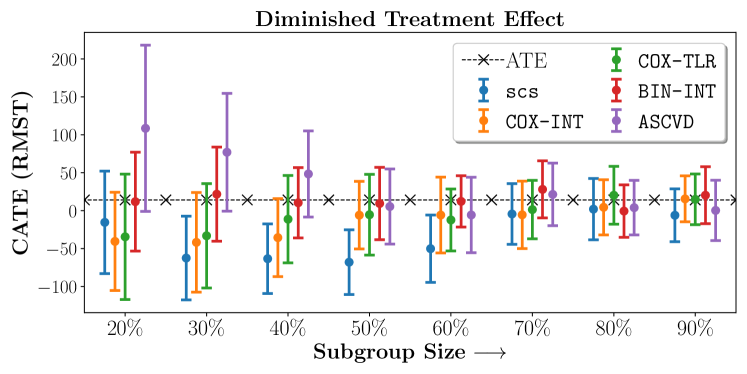
| 20% | 40% | 60% | 80% | |
|---|---|---|---|---|
| SCS | -15.4667.61 | -63.3845.83 | -50.1444.42 | 1.9940.43 |
| COX-INT | -40.5464.8 | -35.5851.4 | -5.8249.97 | 4.4236.41 |
| COX-TLR | -34.5182.71 | -11.2857.62 | -12.340.85 | 20.2838.2 |
| BIN-INT | 11.8465.18 | 10.3946.33 | 12.2333.8 | -0.634.6 |
| ASCVD | 108.54109.62 | 48.3656.77 | -5.749.77 | 3.9336.04 |
| 20% | 40% | 60% | 80% | |
|---|---|---|---|---|
| SCS | 102.4364.9 | 113.9941.35 | 76.4938.53 | 49.7631.25 |
| COX-INT | 74.0463.72 | 57.8250.04 | 50.852.89 | 41.2738.38 |
| COX-TLR | 1.9672.63 | 70.753.71 | 36.5140.91 | 33.9836.9 |
| BIN-INT | 11.8465.18 | 10.3946.33 | 12.2333.8 | -0.634.6 |
| ASCVD | 108.54109.62 | 48.3656.77 | -5.749.77 | 3.9336.04 |