Recruitment dynamics in adaptive social networks
Abstract
We model recruitment in adaptive social networks in the presence of birth and death processes. Recruitment is characterized by nodes changing their status to that of the recruiting class as a result of contact with recruiting nodes. Only a susceptible subset of nodes can be recruited. The recruiting individuals may adapt their connections in order to improve recruitment capabilities, thus changing the network structure adaptively. We derive a mean field theory to predict the dependence of the growth threshold of the recruiting class on the adaptation parameter. Furthermore, we investigate the effect of adaptation on the recruitment level, as well as on network topology. The theoretical predictions are compared with direct simulations of the full system. We identify two parameter regimes with qualitatively different bifurcation diagrams depending on whether nodes become susceptible frequently (multiple times in their lifetime) or rarely (much less than once per lifetime).
pacs:
87.10.Mn, 05.10.GgI Introduction
Any society contains individuals who are carriers of an ideology or fad (e.g., a religious or political party affiliation) that they desire to spread to the rest of the society. Thus, for a given ideology, a society can be partitioned into a set of people that represent the ideology and want to spread it, and the complement of this set. For example, the ideology could correspond to the views of a particular political party, with the party members desiring to recruit new members to improve their positions in the government. Other areas of recruitment have been proposed as mechanisms for fads which appear as a rapid rise above some threshold, as in music Meyer and Ultsch (2010) ,management technologies Bendor et al. (2009), economics Janssen and Jager (2001), and even science Abrahamson (2009) . Slower recruitment based on social networks has been postulated in biology Grueter and Ratnieks (2011) and the spread of alcoholism Benedict (2007). Slowing the rise of a fad or eliminating the spread of an ideology has been also been proposed through the control of critical nodes in a social network Kuhlman et al. (2010).
In today’s world where collisions between ideologies can lead to radicalization of society, the problem of existence and formation of terrorist networks or insurgency movements becomes important. Recently, mathematical modeling of various radical groups, such as terrorist organizations, has been done to explore their structure and dynamics Gutfraind (2009a, b); Johnson et al. (2006); Cherif et al. (2009). In addition to dynamical approaches that measure rates of attacks of radical groups Johnson et al. (2011), operations research theories have also been applied to the formation of radical groups Caulkins et al. (2008). Another class of works Udwadia et al. (2006); Bentson (2006); Butler (2011) focuses on the recruitment dynamics of terrorists within a well-mixed population using compartmental models similar to those used for epidemic spread. In Butler (2011), a systematic analysis of recruitment to Hezbollah has been done. Data from a political science discipline is used to generate a compartmental model of recruitment. Although the modeling is deterministic, it considers the various parameters which explicitly affect the success of recruitment to the radical’s cause. Finally, a number of recent publications discuss terrorist networks as optimal structures that optimize communication efficiency while balancing the secrecy of the networks Lindelauf et al. (2009); Farley (2003); Bar-Isaac and Baccara (2006).
Not considered previously is the combination of the spread of radical ideas plus adaptive changes in social connections to improve recruitment success to the radical cause. Some work in this direction is presented in the papers studying voter models in which individuals make connections to influence others’ opinions Benczik et al. (2008, 2009); Schmittmann and Mukhopadhyay (2010), as well as opinion dynamics models in which individuals are influenced by neighbors’ opinions Holme and Newman (2006).
We develop a simple model of a society in which some of the members belong to a class that tries to spread an ideology. The ideology spreads as a result of contact of recruiting members with nonrecruiting members. The recruiting members may improve their chances to recruit via network adaptation. The purpose of the adaptation proposed here is to improve the spread of the ideology, which is in contrast to network adaptation in epidemiological models Gross et al. (2006); Shaw and Schwartz (2008) where the purpose is avoidance of contact with the spreading members. In addition to adaptation, the connectivity within the society changes due to birth of new members and death of existing members. Using this model, we explore how the existence of stable recruiting classes depends on the adaptation and other parameters. We also consider the network topology of the recruiting class, as it may be important in accessing the quality of the communication channels in the resulting structure. Section II presents the model and a system of mean field equations describing its dynamics. Section III presents mean field analysis of the threshold for successful recruiting and its dependence on the network adaptation. These results are compared with simulations of the full system, and the network geometry of the recruiting class is considered. Section IV concludes.
II Modeling the dynamics of recruitment
II.1 Model
We consider a social structure consisting of individuals represented by nodes in a network. An existing relation between any two individuals is represented by a link between the two nodes. New individuals join the society at a constant total rate , and the individuals in the network can leave the network via death at rate per individual. When new individuals join the system, they arrive with links, which are connected to randomly selected nodes in the population. When individuals die, their links are removed.
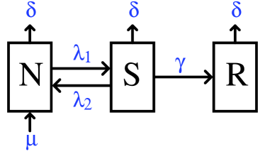
Some members of the society, recruiters (also referred to as R-nodes), are carriers of an ideology that they try to spread to the individuals they come into contact with. The individuals that do not belong to the recruiting class are divided into two groups: those who are susceptible to the recruitment (S-nodes) and those who are non-susceptible (N-nodes). We assume that individuals can spontaneously change their state from non-susceptible to susceptible and vice versa (with rates and respectively). An individual in the recruiting class remains in that class until death Udwadia et al. (2006).
A susceptible individual joins the recruiting class at a rate that is proportional (with proportionality constant ) to the number of contacts it has with the recruiting class. In order to improve their recruiting capabilities, the recruiting individuals can rewire their links with rate , abandoning a connection to a nonsusceptible individual in favor of a connection to a susceptible one. As the links are rewired, the network topology changes based on the current states of its nodes. A schematic representation of the node dynamics is shown on Fig. 1.
We perform Monte Carlo simulations of the above system following the continuous time algorithm described in Gillespie (1976). We start with an Erdos-Renyi random network, which then evolves according to the rules of birth, death, and rewiring. The results presented in the rest of the paper are for the systems that have reached a steady state.
II.2 Mean field
To describe the dynamics of this system, we construct a mean field model for nodes and links as in Gross et al. (2006). The time evolution of the nodes of each type is described by the following rate equations:
| (1a) | ||||
| (1b) | ||||
| (1c) | ||||
Here the functions , , represent the number of nodes of each type. The process of recruitment is captured by the term, where the recruitment is shown to take place at a rate proportional to the number of links between the recruiting class and the susceptible class, .
In order to capture the rewiring process, we follow the evolution of the number of different types of links present in the network:
| (2a) | ||||
| (2b) | ||||
| (2c) | ||||
| (2d) | ||||
| (2e) | ||||
| (2f) | ||||
where the terms correspond to the number of links connecting nodes from classes x and y, e.g., corresponds to the number of NN links. The terms proportional to correspond to the influx of edges due to the birth of new nodes, where the probability for the new node to attach itself to a node from class X is proportional to the number of nodes in that class. The third order terms, , and , describe the formation of triples of nodes with an S-node at the center, and at least one of the edges terminating at an R-node. These terms describe the rate at which NS-, SS- and RS-links become NR-, SR- and RR- links respectively, due to the interaction of the central S-node with its neighboring R-node. Note that our definition of RSR triples includes degenerate triples, i.e., RSR triples where both of the R-nodes correspond to a single R-node, by analogy with degenerate triangles.
The resulting system of equations is not closed, as it contains higher order terms. Following earlier works in epidemiology Keeling et al. (1997), we introduce the closure based on the assumption of homogeneous distribution of RS-links:
| (3a) | ||||
| (3b) | ||||
| (3c) | ||||
We thus obtain a system of nine mean field equations, which we analyze.
III Results
III.1 Mean field recruiting threshold
We first consider the bifurcation point of the recruitment model where the zero recruit (trivial) steady state becomes unstable, which we call the recruiting threshold. This is a transcritical bifurcation point, which is analogous to the epidemic onset in epidemic spreading models. It can be found analytically as a function of parameters for the mean field model, and certain asymptotic limits have a simple form.
We nondimensionalize Eqns. (1) and (2) to simplify the analysis. We introduce the dimensionless time variable , where time is rescaled by the average node lifetime . Further, the node variables are rescaled by the expected population size at steady state, , while the link variables are rescaled by the expected number of links at steady state, . Let denote the 9-dimensional vector of rescaled node and link state variables. Note that in the steady state the rescaled node variables sum to 1, and, therefore, in steady state they correspond to the probability for a node of a given type to exist in the system. Similarly, the rescaled link variables sum to 1, and correspond to the probability for an edge chosen at random to be of a given type, e.g., at steady state corresponds to the probability for a randomly chosen edge to be an RS link.
We introduce the following rescaled parameters:
| (4a) | ||||
| (4b) | ||||
| (4c) | ||||
| (4d) | ||||
We can now write the dimensionless equations of motion as
| (5) |
where is a vector of all the system parameters. (Recall that is a dimensionless integer.) The full system of dimensionless equations is given in Eqs. (11).
We can now find the trivial steady state solution, where the number of R nodes is zero. This restricts the state to be of the form , where the number of links involving R nodes is zero as well. This guarantees that for . Since this subset of equations represents an invariant manifold, we concentrate on solving the equations for the rest of the 5 components, , , , and .
The first observation is that the and equations are solvable when the number of recruiting nodes is zero, and they yield steady state values of
| (6a) | ||||
| (6b) | ||||
| where . The nonzero link variables may be expressed in terms of , and they are given by the following: | ||||
| (6c) | ||||
| (6d) | ||||
| (6e) | ||||
Now that we have the full trivial solution, we can examine its stability. In order to do this, we linearize the vector field about and examine where it has a one dimensional null space. That is, at the bifurcation point, there is only one real eigenvalue passing through zero. This is equivalent to examining where the determinant of the Jacobian vanishes; i.e., we compute those parameters where
| (7) |
The following relation describes the location of the bifurcation:
| (8) |
We next examine the limits of Eq. (8) when either the recruitment rate or rewiring rate is large. The minimum amount of recruitment required to maintain nonzero values of recruited population, when approaches infinity, can be found by setting the least common denominator of Eq. (8) to zero, which yields a simple expression for :
| (9) |
If the recruitment rate is below this value, additional rewiring is not sufficient to enable spreading of the recruiting class.
Similarly, we find the smallest amount of rewiring required for existence of a nontrivial steady state solution, conditioned on our ability to control , with all the other parameters fixed:
For lower rewiring rates, the recruiting class cannot spread even if the recruiting rate is large. The value of this asymptote is greatest, meaning rewiring is most necessary, when approaches zero. In this case few non-susceptible nodes become susceptible to recruiting, and the necessary rewiring value approaches
| (10) |

III.2 Comparison of mean field with simulations
We next compare the mean field predictions for the spread of recruiters with simulations of the full stochastic network system. Thus, we compare the average size of the recruited portion of the population in statistical steady state to the solution of the mean field equations at steady state, which we solve exactly in the Appendix A. We assume that the parameters and (rates for gaining and losing susceptibility) and (determines average degree) depend on details of the society. On the other hand, we assume that the parameters and can be controlled by the recruiters, i.e., the recruiters may choose to be more or less aggressive in their recruitment, as well as in how quickly they rewire their links to susceptible members of society. Therefore, we investigate the recruiting effectiveness for a given choice of , and , while varying and .
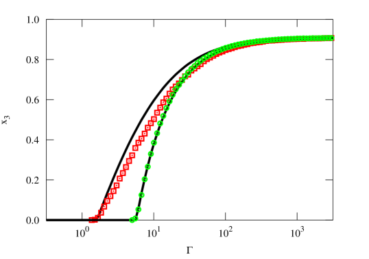
We distinguish two parameter regimes, corresponding to two qualitatively different behaviors of the system: small values of () and large values of (). The small regime corresponds to the case where nodes become susceptible to recruiting only rarely, on average much less than once in their lifetime (where the average lifetime of a node is in the original time units and in the dimensionless units). The large regime corresponds to the case where, on average, nodes become susceptible to recruitment at least once in their lifetime.
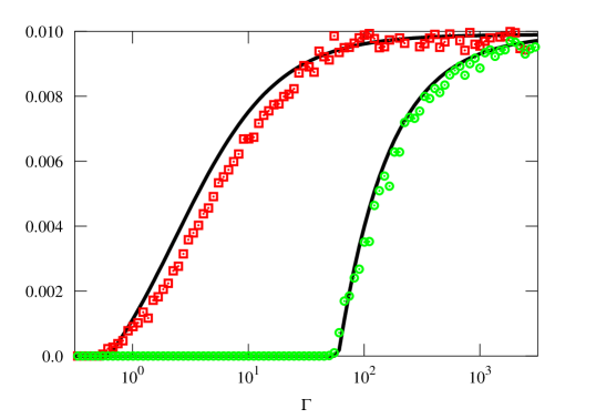
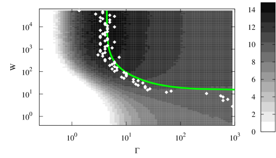
In Figs. 2 and 3 we show the results of simulating the system in these two regimes. The density plots in Figs. 2 and 3 show the fraction of recruited nodes as a function of recruiting rate and rewiring rate in networks with and respectively. The black curves in the two figures represent the location of the recruiting threshold as derived from the mean field equations and given by Eq. (8). Here mean field allows us to accurately predict the onset of the stable nontrivial solution. In Figs. 2 and 3 we compare the simulation results to the mean field predictions. Even though there is some discrepancy between the direct simulations and the mean field near the bifurcation, the recruiting threshold and the asymptotic behavior for large show excellent agreement with the simulations.
We observe in simulations that the steady state trivial solution undergoes a forward transcritical bifurcation in the recruiting rate for all values of for which a nontrivial solution exists. This is in contrast with epidemiological models where the purpose of the rewiring is avoidance of the nodes spreading infection Shaw and Schwartz (2008); Gross et al. (2006), which can undergo a backward transcritical bifurcation and exhibit bistability. Note that, unlike those models, the purpose of the rewiring in the recruitment model is attraction of the susceptible population by the recruiters.
We would like to draw the reader’s attention to an important difference in the system behavior in the two regimes. In the regime where , the nontrivial solution exists for all values of as long as is large enough. On the other hand, in the regime where , the nontrivial solution may fail to exist for any value of unless rewiring is aggressive enough. In Fig. 3 there is a range of rewiring rates for which only trivial solutions exist. The horizontal dashed line, given by Eq. (10), indicates the mean field level of rewiring that is sufficient for the nontrivial solution to exist for rapid recruiting (large ). Also, we can see that the rewiring level that is necessary for the emergence of the nontrivial solution can be very close to the predicted sufficient level of Eq. (10), for small values of .
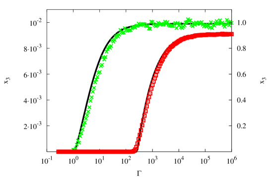
Another important difference between the two regimes of values is seen when we compare two systems with different values of and while the ratio is kept fixed. Note that in the absence of recruitment, such systems have identical fractions of susceptible nodes. In other words, in the presence of recruitment, the pool of individuals available for recruitment would appear to be the same. However, as we can see from Fig. 4, there is a significant difference in the size of the recruited population as well as the recruiting threshold. The difference appears to be caused by the difference in the dynamics in the two regimes. Thus, for the large values of and a node can become susceptible several times during its life, while as the value of decreases, only some nodes will ever become susceptible, with low likelihood of doing so more than once.
III.3 Recruited subnetwork geometry
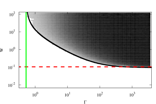
We now investigate the structure of the portion of the network (later referred to as the R-subnetwork) consisting only of R-nodes and links between them. In particular, we are interested in the mean degree of its nodes when the system reaches a steady state. The mean field approach, in addition to predicting the fraction of recruited nodes (which corresponds to the size of the R-subnetwork), also provides information about topology of the subnetwork in the form of mean degree of the nodes. The mean degree of a node in the subnetwork serves as a low order description of how well the nodes in the network are connected, which may be important for communication within the established subnetwork. The density plot in Fig. 5 shows the dependence of the mean degree on and . The nonmonotonic behavior as a function of for fixed is predicted by the mean field model. The solid line corresponds to the analytical prediction of the maximum’s location as given by Eq. (32) derived in Appendix B. Note that the analytic description of the maximum’s location would allow the recruiting class to optimize connectivity within the subnetwork, if that happens to be an important goal for that class. The mean field approximation fails to capture the nonmonotonic behavior of the mean degree in the limit where , and we leave this issue to a future study.
IV Conclusions and Discussion
We develop a toy model that describes recruitment of new members by an interested class within a society. The members of the recruiting class can improve their recruiting capabilities by via adaptation. Thus, they may choose to abandon their relations with those members of society that are not prone to recruitment. This model assumes that once a node joins the recruiting class, it itself becomes a recruiter and it remains a member of this class until death. In contrast to avoidance rewiring used to reduce infection spreading in epidemic models Gross et al. (2006); Shaw and Schwartz (2008), network adaptation in our model promotes spreading. Additionally, the population is open with birth and death modeled explicitly, while most previous adaptive network models have been of closed populations (e.g., Gross et al. (2006); Shaw and Schwartz (2008); Gross and Blasius (2008); Benczik et al. (2008, 2009); Schmittmann and Mukhopadhyay (2010); Holme and Newman (2006)).
In this paper, we develop and analyze a mean field description of our model. Thus, we are able to accurately predict the onset of the stable nontrivial solution of the system at steady state. Furthermore, we are able to accurately predict the size of the recruited class for a given set of system parameters, as well as the mean degree of the subnetwork formed by the recruited members. We compare the predictions made by the mean field description with the direct simulations of our model. We generally observe a good agreement between the model and its mean field approximation.
Analyzing the mean field model, we find two parameter regimes with very distinct qualitative behavior. Thus, we show that in the society where the particular ideology is unpopular (perhaps corresponding to radical ideology) and individuals rarely become susceptible to it, adaptation is necessary in order to observe stable nonzero levels of the recruiting class. On the other hand, if the idea is sufficiently popular (e.g., recruitment into a moderate political party), the adaptation improves the recruiting capabilities and may affect the ultimate topology of the recruited, but adaptation is not a necessary condition for the existence of a nonzero stable solution. Furthermore, we speculate that if the model were changed to describe a society with two competing recruiting classes (think two party system), the adaptation may be a mechanism by which one competing class gets an edge over the other class.
As evidenced by the results presented in Figs. 2 and 3, the mean field approximation has some inaccuracies in the parameter regime between the bifurcation point and the asymptotic saturation. We predict that this inaccuracy is due to errors in the homogeneous closure assumption (Eqs. 3). In a subsequent work, we develop and analyze a new closure of the mean field equations that more accurately describes the full system.
Acknowledgements.
MSS and LBS were supported by the Army Research Office, Air Force Office of Scientific Research, and by Award Number R01GM090204 from the National Institute Of General Medical Sciences. IBS was supported by the Office of Naval Research, the Air Force Office of Scientific Research, and the National Institutes of Health. The content is solely the responsibility of the authors and does not necessarily represent the official views of the National Institute Of General Medical Sciences or the National Institutes of Health.Appendix A Exact solution
In this appendix, we derive the exact solution to the system of equations in Eqs. (1) and (2) when the system is at the nontrivial steady state, i.e., when the left hand side of the equations is zero and the size of recruiting class is nonzero. We begin by deriving the dimensionless equations, as defined in section III.1:
| (11a) | ||||
| (11b) | ||||
| (11c) | ||||
| (11d) | ||||
| (11e) | ||||
| (11f) | ||||
| (11g) | ||||
| (11h) | ||||
| (11i) | ||||
At steady state, the left hand side of the above equations is zero. We proceed in our derivation by dividing all equations in the steady state by and introducing a new variable , obtaining the following system of equations:
| (12a) | ||||
| (12b) | ||||
| (12c) | ||||
| (12d) | ||||
| (12e) | ||||
| (12f) | ||||
| (12g) | ||||
| (12h) | ||||
| (12i) | ||||
We have used the fact that in the steady state , as can be shown by adding together Eqs. (1a)-(1c). In the rest of the derivation we will find a closed equation for and express the other ’s in terms of .
We can immediately express , , and in terms of by solving Eqs. (12b), (12c) and (12i) respectively:
| (13) | ||||
| (14) | ||||
| (15) |
We substitute Eq. (13) into Eq. (12d), and Eq. (14) into Eq. (12g). The resulting two equations, together with Eqs. (12e), (12f) and (12h), form a closed system of five equations with five unknowns -.
We solve Eq. (12f) for in terms of and :
| (16) |
and substitute the above result into Eq. (12d) and (12g), to solve for and in terms of and as follows:
| (17) | ||||
| (18) |
Substituting the expressions for and from Eq. (16) and (17) into Eq. (12e), and solving for we obtain
| (19) |
Finally, substituting results of Eqs. (19) and (18) into Eq. (12h) we obtain an equation for in a closed form:
| (20) |
where
| (21) | ||||
| (22) | ||||
| (23) | ||||
| (24) | ||||
| (25) |
Note that the physically relevant solutions are positive, and therefore finding a nontrivial solution of is a simple matter of solving a quadratic equation:
| (26) |
Solving Eq. (12a) for , we can now express in terms of the newly found :
| (27) |
The rest of the original variables can be found using . Thus, for example, is
| (28) |
Appendix B Extremum of the mean degree in R-subnetwork
In steady state, the mean degree of the nodes within the R-subnetwork is found by taking a ratio of twice the number of RR-links to the number of R-nodes in the subnetwork:
| (29) |
where the values of and are obtained by solving Eqs. (1c) and (2f) in steady state. In this appendix we determine the value of , , that for a given rewiring rate will maximize the degree in the resulting R-subnetwork. We do this by maximizing .
Differentiating Eq. (26) with respect to and evaluating the resulting equation at , the value where extremum is attained, we obtain
| (30) |
Note that the derivative of with respect to evaluated at is equal to zero because is an extremum there, and the are independent of . Multiplying the above equation by and subtracting it from Eq. (26) evaluated at allows us to solve for :
| (31) |
Substituting the value of into Eq. (30) and solving for we obtain
| (32) | |||
the location of the maximum for the given rewiring rate.
References
-
Meyer and Ultsch (2010)
F. Meyer and
A. Ultsch, in
Advances In Data Analysis, Data Handling
And Business Intelligence, German-Classification-Society (German-Classification-Society, 2010), pp. 419–427. - Bendor et al. (2009) J. Bendor, B. A. Huberman, and F. Wu, Journal Of Economic Behavior & Organization 72, 290 (2009).
- Janssen and Jager (2001) M. A. Janssen and W. Jager, Journal Of Economic Psychology 22, 745 (2001).
- Abrahamson (2009) E. Abrahamson, Scandinavian Journal Of Management 25, 235 (2009).
- Grueter and Ratnieks (2011) C. Grueter and F. Ratnieks, Animal Behaviour 81, 949 (2011).
- Benedict (2007) B. Benedict, SIAM News 40 (2007).
-
Kuhlman et al. (2010)
C. Kuhlman,
V. Kumar,
M. Marathe,
S. Ravi, and
D. Rosenkrantz, in
Machine Learning and Knowledge Discovery
in Databases. European Conference,
ECML PKDD 2010. Proceedings (ECML, 2010). - Gutfraind (2009a) A. Gutfraind, Terrorism as a mathematical problem, SIAM News (2009a).
- Gutfraind (2009b) A. Gutfraind, Studies in Conflict and Terrorism 32, 45 (2009b).
- Johnson et al. (2006) N. F. Johnson, M. Spagat, J. A. Restrepo, O. Becerra, J. C. Bohórquez, N. Suárez, E. M. Restrepo, and R. Zarama (2006), http://arxiv.org/abs/physics/0605035.
- Cherif et al. (2009) A. Cherif, H. Yoshioka, W. Ni, and P. Bose (2009), eprint arXiv/0910.5272.
- Johnson et al. (2011) N. Johnson, S. Carran, J. Botner, K. Fontaine, N. Laxague, P. Nuetzel, J. Turnley, and B. Tivnan, SCIENCE 333, 81 (2011), ISSN 0036-8075.
- Caulkins et al. (2008) J. P. Caulkins, D. Grass, D. Feichtinger, and . Tragler, Comp. Oper. Res. 36 (2008).
- Udwadia et al. (2006) F. Udwadia, G. Leitmann, and L. Lambertini, Discrete Dynamics in Nature and Society 2006, 85653 (2006).
- Bentson (2006) K. Bentson, Master’s thesis, Air Force Institute of Technology (2006).
- Butler (2011) L. B. Butler, Tech. Rep. OMB No. 074-0188, SAMS Monograph, Fort Leavenworth, KS 66027-2134 (2011), contains many good references for recruitment, both stochastic and deterministic.
- Lindelauf et al. (2009) R. Lindelauf, P. Borm, and H. Hamers, Social Networks 31, 126 (2009).
- Farley (2003) J. D. Farley, Studies in Conflict and Terrorism 26, 399 (2003).
- Bar-Isaac and Baccara (2006) H. Bar-Isaac and M. Baccara, Working Papers 06-07, New York University, Leonard N. Stern School of Business, Department of Economics (2006), URL http://ideas.repec.org/p/ste/nystbu/06-07.html.
- Benczik et al. (2008) I. J. Benczik, S. Z. Benczik, B. Schmittmann, and R. K. P. Zia, EPL (Europhysics Letters) 82, 48006 (2008).
- Benczik et al. (2009) I. Benczik, S. Benczik, B. Schmittmann, and R. Zia, Physical Review E 79, 046104 (2009).
- Schmittmann and Mukhopadhyay (2010) B. Schmittmann and A. Mukhopadhyay, Phys Rev E Stat Nonlin Soft Matter Phys 82, 066104 (2010).
- Holme and Newman (2006) P. Holme and M. E. J. Newman, Physical Review E 74, 056108 (2006).
- Gross et al. (2006) T. Gross, C. J. D. D’Lima, and B. Blasius, Phys Rev Lett 96, 208701 (2006).
- Shaw and Schwartz (2008) L. Shaw and I. Schwartz, Physical Review E 77, 066101 (2008).
- Gillespie (1976) D. Gillespie, Journal of Computational Physics 22, 403 (1976).
- Keeling et al. (1997) M. J. Keeling, D. A. Rand, and A. J. Morris, Proc Biol Sci 264, 1149 (1997), URL http://dx.doi.org/10.1098/rspb.1997.0159.
- Gross and Blasius (2008) T. Gross and B. Blasius, J R Soc Interface 5, 259 (2008), URL http://dx.doi.org/10.1098/rsif.2007.1229.