Recursive Geman-McClure Estimator for Implementing Second-Order Volterra Filter
Abstract
The second-order Volterra (SOV) filter is a powerful tool for modeling the nonlinear system. The Geman-McClure estimator, whose loss function is non-convex and has been proven to be a robust and efficient optimization criterion for learning system. In this paper, we present a SOV filter, named SOV recursive Geman-McClure, which is an adaptive recursive Volterra algorithm based on the Geman-McClure estimator. The mean stability and mean-square stability (steady-state excess mean square error (EMSE)) of the proposed algorithm is analyzed in detail. Simulation results support the analytical findings and show the improved performance of the proposed new SOV filter as compared with existing algorithms in both Gaussian and impulsive noise environments.
Index Terms:
Adaptive algorithm, Recursive version, Geman-McClure estimator, -stable noise.I Introduction
Adaptive Volterra filters have been thoroughly studied in diverse applications [1, 2, 3, 4]. However, such filters become computationally expensive when a large number of multidimensional coefficients are required. To overcome this problem, many methods were developed [5, 6, 7, 8]. Among these, the second-order Volterra (SOV) filter was widely applied to identify nonlinear system with acceptable error level [9].
The impulsive noise is a great challenge for nonlinear system identification. It has been shown that the impulsive noise could be better modeled by -stable distribution [10]. A symmetric -stable distribution probability density function (PDF) is defined by means of its characteristic function [10] , where is the characteristic exponent, controlling the heaviness of the PDF tails, and is the dispersion, which plays an analogous role to the variance. Such -stable noise tends to produce “outliers”. The recursive least square (RLS), based on the second-order moment, is not robust against outliers [11]. To address stability problem in impulsive noise environments, several RLS-based algorithms were proposed [12, 13, 14]. In [13], a recursive least -norm (RLN) algorithm was proposed. However, this algorithm only achieves improved performance when closes to , where is the order of moments [13]. Another strategy is named as recursive least M-estimate (RLM) algorithm which exploits the M-estimate function to suppress the outliers [14]. Although it is superior to several existing outlier-resistant methods, it suffers from performance degradation in highly impulsive noise environments.
Motivated by these considerations, we employ another M-estimator, named Geman-McClure estimate [15], for nonlinear system identification. Like the estimator, the Geman-McClure estimator is a non-convex M-estimator, which is more efficient for learning system [16]. To the best of our knowledge, no adaptive algorithms can achieve improved performance in both Gaussian and -stable noise environments. By integrating the Geman-McClure estimator in the SOV filter structure, the proposed SOV recursive Geman-McClure algorithm achieves smaller steady-state kernel error as compared with the state-of-art algorithms. Note that a significant reduction is in fact vital from an engineering application perspective. Such a gain would likely justify the increase in computational complexity required to run the proposed algorithm. The fact that a considerable amount of mathematics is needed to derive the algorithms is of no consequence for practical applications, where the cost of hardware principally matters. In this paper, by proper application of mathematical concepts (even if at times cumbersome), we showed that key information about the signal environment could be extracted can be from their observation. Particularly, our main contributions are listed as follows:
(i) The Geman-McClure estimator is first applied in SOV filter for the improved performance in the presence of -stable and Gaussian noises.
(ii) The steady-state behaviour of the proposed algorithm is analyzed.
(iii) We validate the theoretical findings and effectiveness of the proposed algorithm through simulations.
II Problem Formulation
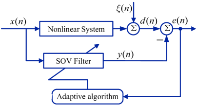
Fig. 1 shows the nonlinear system identification model based on the SOV filter, where and denote the input and output data, denotes the error signal, is the desired signal, and is the noise signal. Given desired signal that satisfies a model of the form
| (1) |
we want to estimate an unknown vector , where denotes the length of the SOV filter. The expanded input vector and the corresponding expanded coefficient vector of the SOV system at time are expressed as
| (2) | ||||
| (3) | |||
where denotes the length of the linear kernel, and stands for the th-order Volterra kernel. Thus, the output of the SOV filter is expressed as
| (4) |
In this case, . In practice, the noise signal may be either Gaussian or non-Gaussian. Hence, it is very clear that efforts make sense in pursuing a more effective SOV-algorithm that satisfies faster convergence and smaller misalignment.
III Proposed algorithm
The conventional Geman-McClure estimator has the following form [15]:
| (5) |
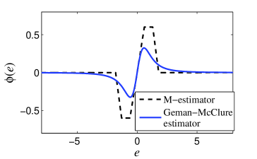
where is a constant that modulates the shape of the loss function. Fig. 2 shows the score functions of the M-estimator and the Geman-McClure estimator, where . It can be observed that for larger values of , the weight updation is small and thus the algorithm is stable in the presence of impulsive noise. For performance improvement, the type of recursive algorithms is usually preferred. Inspired by these merits, the cost function of the proposed algorithm is defined as follows:
| (6) |
where is the forgetting factor. The error signal can be expressed as
| (7) |
Taking the gradient of with respect to the weight vector , and letting the equation be zero, we have
| (8) |
where is the weighting factor. Then, the expression of can be rewritten as:
| (9) |
where , and . If , the above update equation becomes the conventional RLS algorithm. If , and are the weighted autocorrelation matrix and the weighted cross-correlation vector of the optimal weights via . We have to recalculate (9) at each iteration. In our previous studies, an online recursive method is considered to overcome this limitation [11]. By using this approach, and can be adapted by
| (10) |
| (11) |
Using the matrix inversion lemma [17], the adaptation equation of can be obtained as
| (12) |
where , is an identity matrix, is a small positive number, and the gain vector is
| (13) |
Rewriting (9) in a recursive way, we can obtain the following update equation for
| (14) |
Remark 1: In the expression (14), one can see an implicit relationship between and . The algorithm requires an iterative approximation to the optimal solution, where is calculated by using , and the new value for is obtained with the compute the value of .
Remark 2: The proposed algorithm is easy to implement in the SOV filter, since it does not require any priori information on the noise characteristics. It requires two parameters ( and ) to improve the overall nonlinear filtering performance.
IV Performance analysis
In this section, given the Assumptions, we theoretically study the performance of the proposed SOV algorithm. Because the output of the Volterra-based algorithms linearly depend on the coefficients of the filter itself, we can follow the approach in [17, 18] for analyzing the mean performance and steady-state excess mean square error (EMSE) of SOV recursive Gemen-McClure algorithm.
To begin with, we define the weight deviation vector as . In steady-state, the a priori error and the a posterior error are defined as . The mathematical analysis needs the following assumptions.
• Assumptions
a) The input signal is independent and identically distributed (i.i.d.) with zero-mean, and is approximately independent of the a priori error at steady-state, where stands for the squared-weighted Euclidean norm of a vector.
b) The noise signal is i.i.d. with zero-mean and variance .
c) and are mutually independent.
IV-A Mean stability
We can use to rewrite the adaptation equation (14) as
| (15) |
Based on the definition of (12), and using the matrix inversion lemma, we obtain the adaptaion of , which is . Then, we rewrite (15) as
| (16) |
where and . Taking expectations of both sides of (16) and using during the transient state, yields
where denotes the statistical expectation operator. Therefore, the proposed algorithm can converge in the sense of mean if and only if
| (17) |
where is the largest eigenvalue of a matrix. Based on the fact that in (17) 111 is simply not true in the general case. However, if the input signal is persistently exciting, for all infinite and the matrix is nonnegative definite in (17). Hence, we have such inequality., we obtain
| (18) |
Consequently, the mean error weight vector of the proposed algorithm is convergent if the input signal is persistently exciting [17].
IV-B Mean-square stability
Multiplying both sides of (16) by , we have the relationship between the a priori and the a posteriori errors, as below
| (19) |
Using the established energy conservation argument, the proposed algorithm can be expressed as
| (20) |
Combining (16) and (19) and employing as a weighting matrix for the squared-weighted Euclidean norm of a vector, we can get
| (21) |
In the SOV filter with the recursive Geman-McClure algorithm, the adaptive filter will converge to the optimum (minimum) EMSE at steady-state. Therefore, we have
| (22) |
Taking expectations of both sides of (21), and substituting (22) into (21 yields
| (23) |
Substituting (19) into (23) results in
| (24) |
Therefore, in the steady-state (), (24) can be reduced to
| (25) |
Considering Assumption c) and using , the left side of (25) can be expressed as
| (26) | ||||
According to Assumption a), (26) is reduced to
| (27) |
Reusing and considering Assumption b), the right side of (25) can be expressed as
| (28) |
Using (27) and (28), it can be shown that
| (29) |
Eq. (29) can be rewritten as
| (30) |
where and . where is trace operation. Now, let us define the steady-state mean value of as where is the covariance matrix . When the algorithm is close to the optimal EMSE. In this case, can be approximated as
| (31) |
For , we have at steady-state. Finally, substituting (31) and into (30), we arrive at
| (32) |
where . Note that it is very hard to further simplify (32). The theoretical result contains a random variable , but after the expect operation, we can obtain an exact value. Furthermore, (32) is also applicable to the analysis of linear recursive Geman-McClure algorithm.
Finally, we compare the computational complexities of the algorithms, as shown in Table I, where denotes the length of sliding-window in the SOV-RLM algorithm. The arithmetic complexity of the proposed algorithm is comparable to that of the SOV-RLS algorithm, except for the more multiplications, 1 addition and 1 division in (13).
| Algorithms | Multiplications | Additions | Other operations |
|---|---|---|---|
| SOV-RLS | 1 division | ||
| SOV-RLM | 1 division and | ||
| SOV-RLN | 2 divisions and -power operation | ||
| Proposed algorithm | 2 divisions |
V Simulation results
To verify the theoretical findings and to illustrate the effectiveness of the proposed algorithm, we present simulations when implemented in Matlab R2013a running on a 2.1GHz AMD processor with 4GB of RAM. The EMSE and normalized mean square deviation (NMSD) are employed to evaluate the performance. The results are averaged over 300 independent simulations.
V-A Gaussian scenarios
| SNR | EMSE | |||
|---|---|---|---|---|
| Theory | Simulation | |||
| 25dB | 0.5 | 14 [11] | 36.66dB | 36.75dB |
| 40dB | 1.8 | 14 [11] | 51.64dB | 51.83dB |
| 20dB | 0.2 | 14 [18] | 32.27dB | 31.77dB |
| 30dB | 0.45 | 14 [18] | 41.70dB | 41.83dB |
| 10dB | 0.9 | 20 [19] | 20.65dB | 20.14dB |
| 30dB | 0.6 | 20 [19] | 39.83dB | 40.40dB |
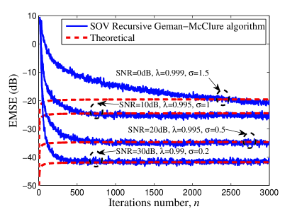
In this example, we provide simulation verification for the analysis. The Gaussian distribution with zero-mean and unit variance is adopted to generate and . Fig. 3 plots the simulation and theoretical results of the EMSEs for different signal-to-noise ratio (SNR) and parameter settings. The unknown plant is a 14-tap nonlinear system, which is presented by [11]. It is observed that the simulations agree well with the analysis results in all scenarios. Next, we compare the theoretical and the simulation results of the steady-state EMSEs for different unknown systems. The input and noise signals used have similar characteristics as in Fig. 3. The unknown parameter vector has or entries and is defined by [18, 19]. Table II provides the simulation and theoretical EMSE values with different Volterra systems. This shows agreements in the SOV filter in spite of different SNRs, parameter settings and unknown systems. The difference between simulation results and theory arises from some approximations and assumptions used for deriving (32).
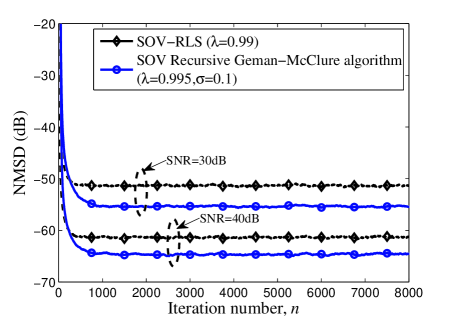
We compare the convergence rate and steady-state kernel behaviour of the proposed algorithm with existing algorithms. The unknown system is a 14-tap nonlinear system [11]. A zero-mean white Gaussian noise (WGN) is used as the input signal. We observe that the proposed algorithm outperforms the standard SOV-RLS algorithm by nearly 5dB in steady-state where the noise signal is WGN with different SNRs (Fig. 4).
V-B Non-Gaussian scenarios
|
|---|
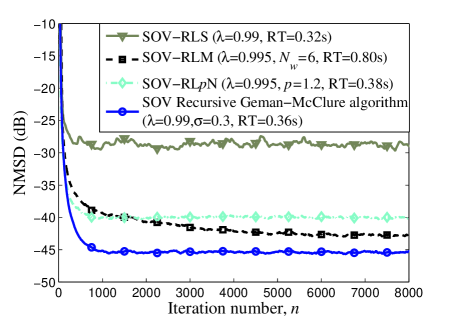
In the second example, we repeat the same simulations as above, but this time using -stable noise as the noise signal. First, we study the effect of on the performance of the SOV recursive Geman-McClure algorithm under the impulsive noise. For sake of fair comparison, we use the same fixed forgetting factor to obtain a similar convergence rate. The results are shown in Table III. It is indicated that the performance deteriorates quickly with the increasing of when is greater than 0.4. For an overall consideration of steady-state NMSD performance and convergence rate, the best choice is in this example. Hence, we fix in following simulations. Fig. 5 illustrates the NMSD performance of algorithms in the presence of -stable noise. One can also see that in impulsive noise scenario, the proposed SOV recursive Geman-McClure algorithm achieves better performance than its SOV-based counterparts 222The SOV-RLM and SOV-RLN algorithms can be derived by extending algorithms [13, 14] to the SOV filter structure.. In the legend of the figure, we use the RT to denote the run time for algorithm. It can be seen that the run time of the proposed algorithm fall in between the RLS and RLN. Since the proposed algorithm achieves improved performance in both cases, we can conclude that the SOV recursive Geman-McClure algorithm has robust performance for various scenarios and is an excellent alternative to the SOV-RLS algorithm for nonlinear system identification task.
VI Conclusion
In this paper, we proposed a recursive Geman-McClure algorithm based on SOV filter, which was derived by minimizing the Geman-McClure estimator of the error signal. Detailed steady-state analysis was presented. One of the advantages of the proposed algorithm is that it has only two parameters, the constant and the forgetting factor , which have quite wide ranges for choice to achieve excellent performance. We carried out computer simulations that support the analytical findings and confirm the effectiveness of the proposed algorithm. Note that the variance of -stable noise is infinite, so it is very difficult, if not impossible, to conduct a steady-state performance analysis of the proposed algorithm. Similarly, theoretical analysis of global stability and convergence is also very hard and rare for the Volterra filters in the presence of -stable noise. Rigorous mathematical analysis is lacking in a long period. We leave these investigations for future work.
References
- [1] O. Karakuş, E. Kuruoğlu, and M. A. Altınkaya, “Bayesian Volterra system identification using reversible jump MCMC algorithm,” Signal Process., vol. 141, pp. 125–136, 2017.
- [2] N. Mallouki, B. Nsiri, S. Mhatli, M. Ghanbarisabagh, W. Hakimi, and M. Ammar, “Analysis of full Volterra and sparse Volterra nonlinear equalization for downlink LTE system,” Wireless Pers. Commun., vol. 89, no. 4, pp. 1413–1432, 2016.
- [3] G. L. Sicuranza and A. Carini, “Filtered-X affine projection algorithm for multichannel active noise control using second-order Volterra filters,” IEEE Signal Process. Lett., vol. 11, no. 11, pp. 853–857, 2004.
- [4] ——, “A multichannel hierarchical approach to adaptive Volterra filters employing filtered-X affine projection algorithms,” IEEE Trans. Signal Process., vol. 53, no. 4, pp. 1463–1473, 2005.
- [5] E. L. Batista and R. Seara, “A reduced-rank approach for implementing higher-order Volterra filters,” EURASIP J. Adv. Signal Process., vol. 2016, no. 1, p. 118, 2016.
- [6] S. Wang, Y. Zheng, S. Duan, L. Wang, and K. T. Chi, “A class of improved least sum of exponentials algorithms,” Signal Process., vol. 128, pp. 340–349, 2016.
- [7] B. Chen, J. Liang, N. Zheng, and J. C. Príncipe, “Kernel least mean square with adaptive kernel size,” Neurocomputing, vol. 191, pp. 95–106, 2016.
- [8] M. Scarpiniti, D. Comminiello, R. Parisi, and A. Uncini, “Spline adaptive filters: Theory and applications,” in Adaptive Learning Methods for Nonlinear System Modeling. Elsevier, 2018, pp. 47–69.
- [9] T. Ogunfunmi, Adaptive Nonlinear System Identification: The Volterra and Wiener Based Approaches. New York, NY, USA: Springer-Verlag, 2007.
- [10] M. Shao and C. L. Nikias, “Signal processing with fractional lower order moments: stable processes and their applications,” Proc. IEEE, vol. 81, no. 7, pp. 986–1010, 1993.
- [11] L. Lu, H. Zhao, and B. Chen, “Improved-variable-forgetting-factor recursive algorithm based on the logarithmic cost for Volterra system identification,” IEEE Trans. Circuits Syst. II, vol. 63, no. 6, pp. 588–592, 2016.
- [12] A. Singh and J. C. Príncipe, “A closed form recursive solution for maximum correntropy training,” in Proc. ICASSP. IEEE, 2010, pp. 2070–2073.
- [13] A. Navia-Vazquez and J. Arenas-Garcia, “Combination of recursive least -norm algorithms for robust adaptive filtering in alpha-stable noise,” IEEE Trans. Signal Process., vol. 60, no. 3, pp. 1478–1482, 2012.
- [14] Y. Zou, S. Chan, and T. Ng, “Robust M-estimate adaptive filtering,” IEE Proc. Vision, Image, Signal Process., vol. 148, no. 4, pp. 289–294, 2001.
- [15] K. Li and J. Malik, “Learning to optimize,” arXiv:1606.01885, 2016.
- [16] F. D. Mandanas and C. L. Kotropoulos, “Robust multidimensional scaling using a maximum correntropy criterion,” IEEE Trans. Signal Process., vol. 65, no. 4, pp. 919–932, 2017.
- [17] A. H. Sayed, Fundamentals of Adaptive Filtering. John Wiley & Sons, 2003.
- [18] J. Lee and V. J. Mathews, “A fast recursive least squares adaptive second order Volterra filter and its performance analysis,” IEEE Trans. Signal Process., vol. 41, no. 3, pp. 1087–1102, 1993.
- [19] S. Kalluri and G. R. Arce, “A general class of nonlinear normalized adaptive filtering algorithms,” IEEE Trans. Signal Process., vol. 47, no. 8, pp. 2262–2272, 1999.