Recursive variational Gaussian approximation with the Whittle likelihood for linear non-Gaussian state space models
Abstract
Parameter inference for linear and non-Gaussian state space models is challenging because the likelihood function contains an intractable integral over the latent state variables. While Markov chain Monte Carlo (MCMC) methods provide exact samples from the posterior distribution as the number of samples go to infinity, they tend to have high computational cost, particularly for observations of a long time series. Variational Bayes (VB) methods are a useful alternative when inference with MCMC methods is computationally expensive. VB methods approximate the posterior density of the parameters by a simple and tractable distribution found through optimisation. In this paper, we propose a novel sequential variational Bayes approach that makes use of the Whittle likelihood for computationally efficient parameter inference in this class of state space models. Our algorithm, which we call Recursive Variational Gaussian Approximation with the Whittle Likelihood (R-VGA-Whittle), updates the variational parameters by processing data in the frequency domain. At each iteration, R-VGA-Whittle requires the gradient and Hessian of the Whittle log-likelihood, which are available in closed form for a wide class of models. Through several examples using a linear Gaussian state space model and a univariate/bivariate non-Gaussian stochastic volatility model, we show that R-VGA-Whittle provides good approximations to posterior distributions of the parameters and is very computationally efficient when compared to asymptotically exact methods such as Hamiltonian Monte Carlo.
Keywords: Autoregressive process; Fast Fourier transform; Hamiltonian Monte Carlo; Stationary time series; Stochastic volatility models.
1 Introduction
State space models (SSMs) are a widely used class of hierarchical time series models employed in a diverse range of applications in fields such as epidemiology (e.g., Dukic et al.,, 2012), economics (e.g., Chan and Strachan,, 2023), finance (e.g., Kim et al.,, 1998), and engineering (e.g., Gordon et al.,, 1993). In an SSM, the observed data depend on unobserved, time-evolving latent state variables and unknown parameters. The observations are assumed to be conditionally independent given the latent states, the dynamics of the latent states are described through a Markov process, and often a simplifying assumption of linearity of the state variables is made. When the state variables are non-Gaussian, Bayesian inference for the parameters of these SSMs is challenging since the likelihood function involves an intractable integral over the latent states.
A popular class of inference methods for non-Gaussian SSMs is Markov chain Monte Carlo (MCMC). While MCMC methods can provide samples from the posterior distribution that are asymptotically exact, they tend to be computationally expensive. An early application of MCMC to nonlinear, non-Gaussian state-space models (SSMs) is the work of Meyer et al., (2003), which combines the Laplace approximation (Laplace,, 1986) and the extended Kalman filter (Harvey,, 1990) to approximate the likelihood function. This approximation is then used within a Metropolis-Hastings algorithm to estimate parameters in a nonlinear, non-Gaussian stochastic volatility model. While this likelihood approximation is analytical, it is only exact for linear, Gaussian SSMs. An alternative approach is the pseudo-marginal Metropolis-Hastings algorithm developed by Andrieu and Roberts, (2009), which employs an unbiased likelihood estimate obtained through a particle filter. However, particle filters are computationally intensive and prone to particle degeneracy, especially when dealing with large datasets (see Kantas et al., (2009) for a detailed discussion of this issue). Both approaches typically require many iterations, each involving a full data pass with complexity , where is the number of observations, making them costly for long data sequences. Additionally, other alternatives, such as the Hamiltonian Monte Carlo (HMC) method (Duane et al.,, 1987; Neal,, 2011; Hoffman and Gelman,, 2014), target the joint posterior distribution of states and parameters and typically require many iterations to achieve parameter convergence when is large and the state dimension is high.
Variational Bayes (VB) methods are becoming increasingly popular for Bayesian inference for state space models (Zammit-Mangion et al.,, 2012; Gunawan et al.,, 2021; Frazier et al.,, 2023). VB approximates the posterior distribution of model parameters with a simpler and more tractable class of distributions constructed using so-called variational parameters, which are unknown and estimated via optimisation techniques. While VB methods tend to be more computationally efficient than MCMC methods, they provide approximate posterior distributions. For a review of VB methods, see Blei et al., (2017).
There are two main classes of VB methods: batch and sequential. A batch VB framework (e.g., Tran et al.,, 2017; Tan and Nott,, 2018; Loaiza-Maya et al.,, 2022; Gunawan et al.,, 2024) requires an optimisation algorithm to repeatedly process the entire dataset until variational parameters converge to a fixed point. A sequential VB framework, on the other hand, updates variational parameters using one observation at a time. Sequential methods only pass through the entire dataset once, and are thus ideal for settings with large datasets. Sequential VB methods are available for statistical models for independent data (Lambert et al.,, 2022), for classical autoregressive models for time-series data (Tomasetti et al.,, 2022), for generalised linear mixed models (Vu et al.,, 2024), and for SSMs where the state evolution model is linear and Gaussian (Beal,, 2003, Chapter 5; Zammit Mangion et al.,, 2011; Mangion et al.,, 2011). Campbell et al., (2021) proposed a sequential VB approach that is applicable to an SSM with non-linear state dynamics and non-Gaussian measurement errors, but this approach can be computationally expensive as it requires solving an optimisation problem and a regression task for each time step.
Our article proposes a sequential VB approach to estimate parameters in linear non-Gaussian state space models. This approach builds on the Recursive Variational Gaussian Approximation (R-VGA) algorithm of Lambert et al., (2022). We first transform time-domain data into frequency-domain data and then use the Whittle likelihood (Whittle,, 1953) in a sequential VB scheme. The logarithm of the Whittle likelihood function is a sum of the individual log-likelihood components in Fourier space, and is thus well-suited for use in sequential updating. We call our algorithm the Recursive Variational Gaussian Approximation with the Whittle likelihood (R-VGA-Whittle) algorithm. At each iteration, R-VGA-Whittle sequentially updates the variational parameters by processing one frequency or a block of frequencies at a time. Although sequential in nature, and requiring only one pass through the frequencies, we note that the R-VGA-Whittle algorithm requires the full dataset to be available in order to construct the periodogram, from which we obtain the frequency-domain data.
We demonstrate the performance of R-VGA-Whittle in simulation studies involving a linear Gaussian state space model and univariate and bivariate non-Gaussian stochastic volatility models. We show that R-VGA-Whittle is accurate and is much faster than HMC with the exact likelihood as well as HMC based on the Whittle likelihood; hereafter, we refer to these two methods as HMC-exact and HMC-Whittle, respectively. We subsequently apply R-VGA-Whittle to analyse exchange rate data.
The rest of the article is organised as follows. Section 2 gives an overview of SSMs and the univariate and multivariate Whittle likelihood functions, and then introduces the R-VGA-Whittle and HMC-Whittle algorithms. Section 3 compares the performance of R-VGA-Whittle, HMC-Whittle and HMC with the exact likelihood in several examples involving linear Gaussian and non-Gaussian SSMs. Section 4 summarises and discusses our main findings. The article also has an online supplement with additional technical details and empirical results.
2 Methodology
We give an overview of SSMs in Section 2.1, and the univariate and multivariate Whittle likelihoods in Section 2.2. Section 2.3 introduces R-VGA-Whittle, while Section 2.4 proposes a blocking approach to improve computational efficiency. Section 2.5 gives details of HMC-Whittle.
2.1 State space models
An SSM consists of two sub-models: a data model that describes the relationship between the observations and the latent state variables, and a state evolution model that describes the (temporal) evolution of the latent states.
In SSMs, the -dimensional latent state variables are characterised by an initial density and state transition densities
| (1) |
where is a vector of model parameters. The observations are related to the latent states via
| (2) |
where each is assumed to be conditionally independent of the other observations, when conditioned on the latent state . A linear SSM is one where and in (1) and (2) can each be expressed as the sum of two components: a linear function of their conditioning variables and an exogenous random component.
Let and be vectors of observations and latent states, respectively. The posterior density of the model parameters is , where the likelihood function is
This likelihood function is intractable, except for special cases such as the linear Gaussian SSM (e.g., Gibson and Ninness,, 2005). In non-Gaussian SSMs, the likelihood is typically estimated using a particle filter (Gordon et al.,, 1993), such as in the pseudo-marginal Metropolis-Hastings (PMMH) method of Andrieu and Roberts, (2009), which can be computationally expensive for large .
The Whittle likelihood (Whittle,, 1953) is a frequency-domain approximation of the exact likelihood, and offers a computationally efficient alternative for parameter inference in SSMs. Transforming the data to the frequency domain “bypasses” the need for integrating out the states when computing the likelihood, as the Whittle likelihood only depends on the model parameters and not the latent variables. In the following sections, we review the Whittle likelihood and its properties, and then propose a sequential VB approach that uses the Whittle likelihood for parameter inference.
2.2 The Whittle likelihood
The Whittle likelihood has been widely used to estimate the parameters of complex time series or spatial models. It is more computationally efficient to evaluate than the exact likelihood, although it is approximate (e.g., Sykulski et al.,, 2019). Some applications of the Whittle likelihood include parameter estimation with long memory processes (e.g., Robinson,, 1995; Hurvich and Chen,, 2000; Giraitis and Robinson,, 2001; Abadir et al.,, 2007; Shao and Wu, 2007b, ; Giraitis et al.,, 2012), and with spatial models with irregularly spaced data (e.g., Fuentes,, 2007; Matsuda and Yajima,, 2009). The Whittle likelihood is also used for estimating parameters of vector autoregressive moving average (VARMA) models with heavy-tailed errors (She et al.,, 2022), and of vector autoregressive tempered fractionally integrated moving average (VARTFIMA) models (Villani et al.,, 2022).
2.2.1 Univariate Whittle likelihood
Consider a real-valued, zero-mean, second-order stationary, univariate time series with autocovariance function , where and is the expectation operator. The power spectral density of the time series is the Fourier transform of the autocovariance function (Brillinger,, 2001):
| (3) |
where is the angular frequency and is a vector of model parameters. The periodogram, an asymptotically unbiased estimate of the spectral density, is given by
| (4) |
where , and is the discrete Fourier transform (DFT) of :
| (5) |
For an observed time series, the Whittle likelihood, denoted by , is (e.g., Salomone et al.,, 2020)
| (6) |
Here, the Whittle likelihood is evaluated by summing over the non-negative frequencies only, since and are both symmetric about the origin for real-valued time series. The term is not included since when the time series is de-meaned. The term is also omitted since it has a different distribution from the other frequencies and its influence is asymptotically negligible (Salomone et al.,, 2020; Villani et al.,, 2022).
Asymptotically, it can be shown that the parameter estimates obtained by maximising the exact likelihood and those obtained by maximising the Whittle likelihood are equivalent (Dzhaparidze and Yaglom,, 1983). The calculation of the Whittle likelihood involves evaluation of the periodogram, which does not depend on the parameters and can, therefore, be pre-computed at a cost of via the Fast Fourier Transform (FFT, Cooley and Tukey,, 1965). Since the periodogram ordinates are asymptotically independent (Whittle,, 1953), the logarithm of the Whittle likelihood is a sum of the individual log-likelihood terms computed over different frequencies.
2.2.2 Multivariate Whittle likelihood
Consider a -variate, real valued, second-order stationary, zero mean time series with autocovariance function , . At a given angular frequency , the power spectral density matrix of this series is
| (7) |
The matrix-valued periodogram is
| (8) |
where , denotes the conjugate transpose of a complex matrix , and , the DFT of the series, is given by
| (9) |
The Whittle likelihood for the multivariate series is (Villani et al.,, 2022):
| (10) |
2.3 R-VGA-Whittle
The original R-VGA algorithm of Lambert et al., (2022) is a sequential VB algorithm for parameter inference in statistical models where the observations are independent, such as linear or logistic regression models. Given independent and exchangeable observations , this algorithm sequentially approximates the “pseudo-posterior” distribution of the parameters given data up to the th observation, , with a Gaussian distribution . The updates for and are available in closed form, as seen in Algorithm 1. We describe this algorithm in more detail in Section S1 of the online supplement.
At each iteration , the R-VGA algorithm requires the gradient and Hessian of the log-likelihood contribution from each observation, . In a setting with independent observations, these likelihood contributions are easy to obtain; however, in SSMs where the latent states follow a Markov process and are hence temporally dependent, the log-likelihood function is intractable, as shown in Section 2.1. The gradient and Hessian of , , are hence also intractable. While these quantities can be estimated via particle filtering (e.g., Doucet and Shephard,, 2012), one would need to run a particle filter from the first time period to the current time period for every step in the sequential algorithm. This quickly becomes infeasible for long time series.
We now extend the R-VGA algorithm of Lambert et al., (2022) to state space models by replacing the time domain likelihood with a frequency domain alternative: the Whittle likelihood. From (6) and (10) we see that the log of the Whittle likelihood is a sum over individual log-likelihood components, a consequence of the asymptotic independence of the periodogram frequency components (Shao and Wu, 2007a, ). We replace the quantities and in Algorithm 1 with the gradient and Hessian of the Whittle log-likelihood evaluated at each frequency. In the univariate case, the individual log-likelihood contribution at frequency is
| (11) |
while in the multivariate case,
| (12) |
for . The log-likelihood contributions are available for models where the power spectral density is available analytically, such as models where the latent states follow a VARMA (She et al.,, 2022) or a VARTFIMA (Villani et al.,, 2022) process. The gradient and Hessian are therefore also available in closed form for these models. At each VB update, and are used to update the variational parameters for . Their expectations with respect to are approximated using Monte Carlo samples , :
for . We set following an experiment on the sensitivity of the algorithm to the choice of ; see Section S4 of the online supplement for more details.
We also implement the damping approach of Vu et al., (2024) to mitigate instability that may arise when traversing the first few frequencies. Damping is done by splitting an update into steps, where is user-specific. In each step, the gradient and the Hessian of the log of the Whittle likelihood are multiplied by a “step size” , and the variational parameters are updated times during one VB iteration. This has the effect of splitting a log-likelihood contribution into “parts”, and using them to update variational parameters one part at a time. In practice, we set through experimentation, and choose it so that initial algorithmic instability is reduced with only a small increase in computational cost. We summarise R-VGA-Whittle in Algorithm 2.
2.4 R-VGA-Whittle with block updates
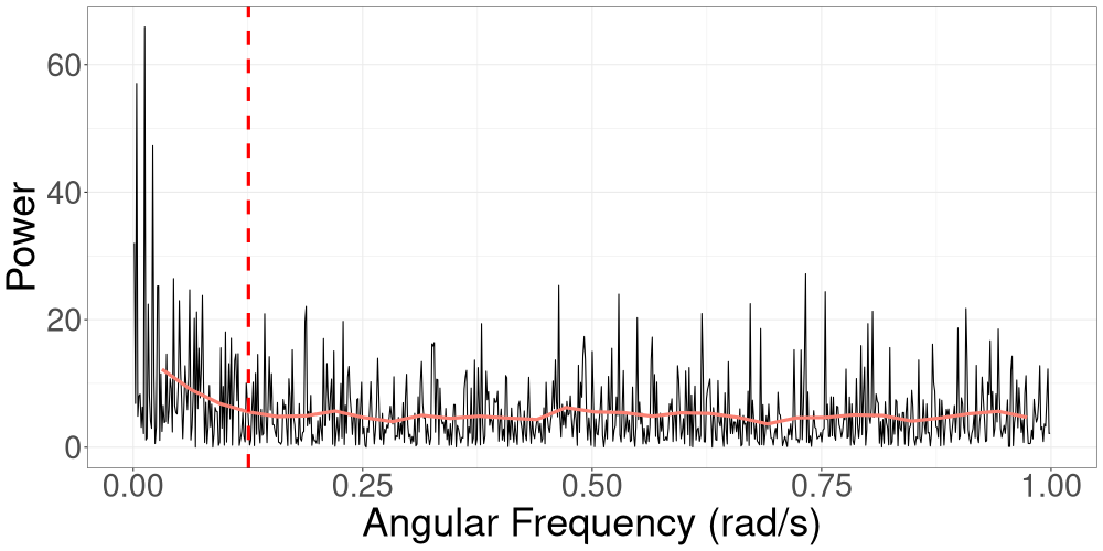
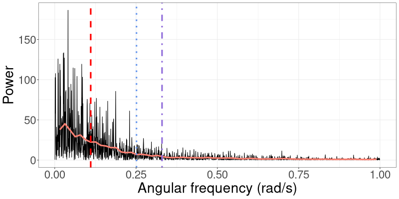
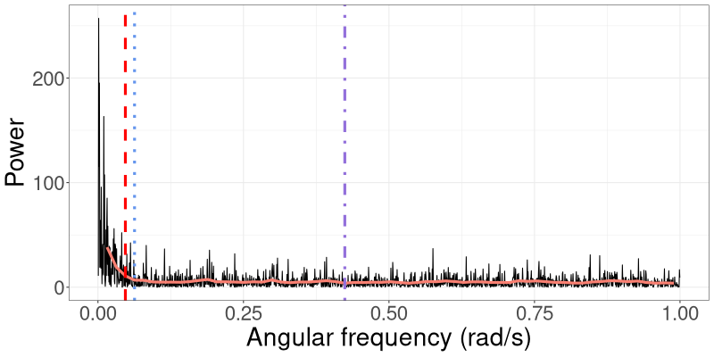
The spectral density of a process captures the distribution of signal power (variance) across frequency (Percival and Walden,, 1993). The periodogram is an estimate of the spectral density. In Figure 1(a), we show the periodogram for data generated from the linear Gaussian SSM that we consider in Section 3.1. The variance (power) of the signal gradually decreases as the frequency increases, which means that lower frequencies contribute more to the total power of the process. A similar pattern is seen in Figure 1(b), which shows the periodogram for data generated from a univariate stochastic volatility model that we consider in Section 3.2. In this case there is an even larger concentration of power at the lower frequencies.
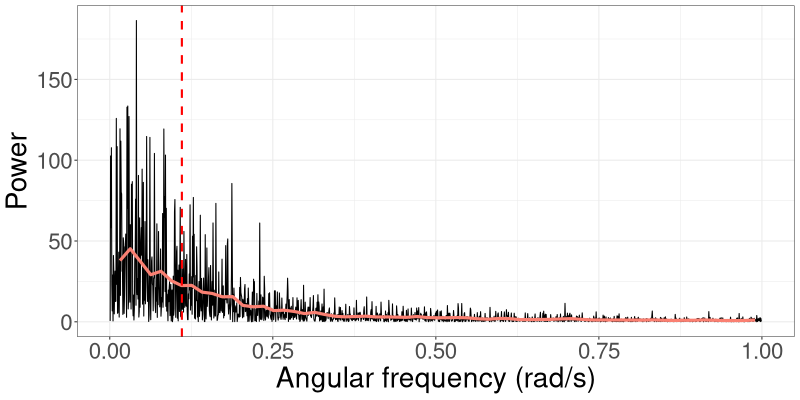
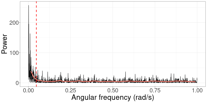
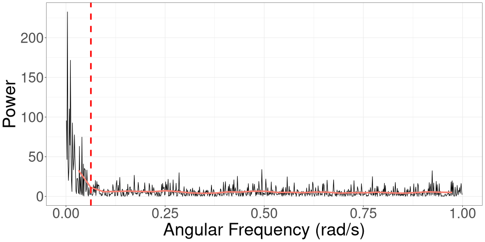
Frequencies that carry less power have less effect on R-VGA-Whittle updates. To speed up the algorithm and reduce the number of gradient/Hessian calculations, we therefore process angular frequency contributions with low power, namely those beyond the 3dB cutoff point, together in “blocks”. We define the 3dB cutoff point as the angular frequency at which the power drops to half the maximum power in the (smoothed) periodogram, which we obtain using Welch’s method (Welch,, 1967). Section S3 studies several cutoff points and empirically justifies our choice of a 3dB cutoff.
Assume the 3dB cutoff point occurs at ; we split the remaining angular frequencies into blocks of approximately equal length . Suppose that there are blocks, with , denoting the set of angular frequencies in the th block. The variational mean and precision matrix are then updated based on each block’s Whittle log-likelihood contribution. For , this is given by
| (13) |
that is, by the sum of the Whittle log-likelihood contributions of the frequencies in the block.
For a multivariate time series, we compute the periodogram for each individual time series along with its corresponding 3dB cutoff point, and then use the highest cutoff point in R-VGA-Whittle. An example of bivariate time series periodograms along with their 3dB cutoffs points is shown in Figure 2.
We summarise R-VGA-Whittle with block updates in Algorithm 3.
2.5 HMC-Whittle
We now discuss the use of HMC with the Whittle likelihood for estimating parameters in SSMs. Suppose we want to sample from the posterior distribution . We introduce an auxiliary momentum variable of the same length as and assume comes from a density , where is a mass matrix that is often a multiple of the identity matrix. The joint density of and is , where
| (14) |
is called the Hamiltonian, and . HMC proceeds by moving and according to the Hamiltonian equations
| (15) |
to obtain new proposed values and . By Bayes’ theorem, , so the gradient can be written as
| (16) |
The gradient on the right hand side of (16) is typically intractable in SSMs and needs to be estimated using a particle filter (e.g., Nemeth et al.,, 2016). However, if the exact likelihood is replaced with the Whittle likelihood, an approximation to can be obtained without the need for running an expensive particle filter repeatedly. Rather than targeting the true posterior distribution , HMC-Whittle proceeds by targeting an approximation , where is the Whittle likelihood as defined in (6) for a univariate time series, or (10) for multivariate time series. Then in (14) is replaced by the quantity , and the term in (15) is replaced with
| (17) |
For models where the spectral density is available in closed form, the Whittle likelihood is also available in closed form, and the gradient can be obtained analytically.
In practice, the continuous-time Hamiltonian dynamics in (15) are simulated over discrete time steps of size using a leapfrog integrator (see Algorithm 4). The resulting and from this integrator are then used as proposals and are accepted with probability
This process of proposing and accepting/rejecting is repeated until the desired number of posterior samples has been obtained. We summarise HMC-Whittle in Algorithm 5.
3 Applications
This section demonstrates the use of R-VGA-Whittle for estimating parameters of a univariate linear Gaussian SSM and those of a univariate/bivariate stochastic volatility (SV) model using simulated and real data. We compare the posterior densities obtained from R-VGA-Whittle to those from HMC-exact and HMC-Whittle. All examples are implemented in R, and the reproducible code is available from https://github.com/bao-anh-vu/R-VGA-Whittle. HMC-exact and HMC-Whittle are implemented using the CmdStanR interface to the Stan programming language (Gabry et al.,, 2024).
For all examples, we implement R-VGA-Whittle with damping and blocking as described in Algorithm 3. We apply damping to the first angular frequencies with damping steps each. These values were chosen to reduce the initial instability at the expense of a small additional computational cost. We select for each model by finding the 3dB frequency cutoff and process the remaining frequencies in blocks of length , following a study in Section S3 of the online supplement. At each iteration of R-VGA-Whittle, we use Monte Carlo samples to approximate the expectations of the gradient and Hessian of the Whittle log-likelihood. This value of was chosen because it results in very little variation between repeated runs of R-VGA-Whittle; see Section S4 of the online supplement for an experiment exploring the algorithm’s sensitivity to . HMC-Whittle and HMC-exact were run with two chains with 15000 samples each. The first 5000 samples of each chain were discarded as burn-in. All experiments were carried out on a high-end server, with an NVIDIA Tesla V100 32GB graphics processing unit (GPU) used to parallelise over the Monte Carlo samples needed for estimating the expectations of the gradient and Hessian of the Whittle log-likelihood at each iteration of Algorithm 2.
3.1 Univariate linear Gaussian SSM
We generate observations from the linear Gaussian SSM,
| (18) | ||||
| (19) | ||||
| (20) |
We set the true auto-correlation parameter to , the true state disturbance standard deviation to and the true measurement error standard deviation to .
The parameters that need to be estimated, and , take values in subsets of . We therefore instead estimate the transformed parameters , where , , and , which are unconstrained.
The spectral density of the observed time series is
| (21) |
where
is the spectral density of the AR(1) process , and
is the spectral density of the white noise process . The Whittle log-likelihood for this model is given by (6), where the periodogram is the discrete Fourier transform (DFT) of the observations , which we compute using the fft function in R. We evaluate the gradient and Hessian of the Whittle log-likelihood at each frequency, and , using automatic differentiation via the tensorflow library (Abadi et al.,, 2015) in R. The initial/prior distribution we use is
| (22) |
This leads to 95% probability intervals of for , and for and .
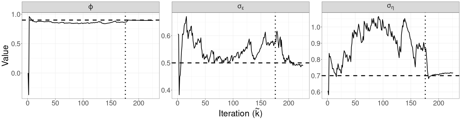
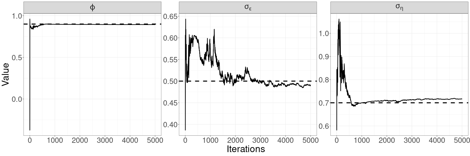
Figure 3 shows the trajectory of the R-VGA-Whittle variational mean for each parameter. There are only 226 R-VGA-Whittle updates, as the 3dB cutoff point is the 176th angular frequency, and there are 50 blocks thereafter. The figure shows that the trajectory of moves towards the true value within the first 10 updates. This is expected, since most of the information on , which is reasonably large in our example, is in the low-frequency components of the signal. The trajectories of and are more sporadic before settling close to the true value around the last 25 (block) updates. This later convergence is not unexpected since high-frequency log-likelihood components contain non-negligible information on these parameters that describe fine components of variation (the spectral density of white noise is a constant function of frequency). This behaviour is especially apparent for the measurement error standard deviation .
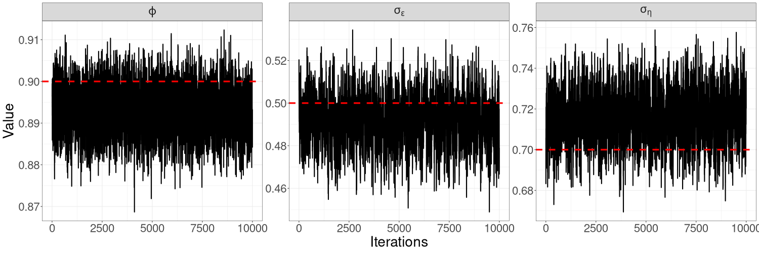
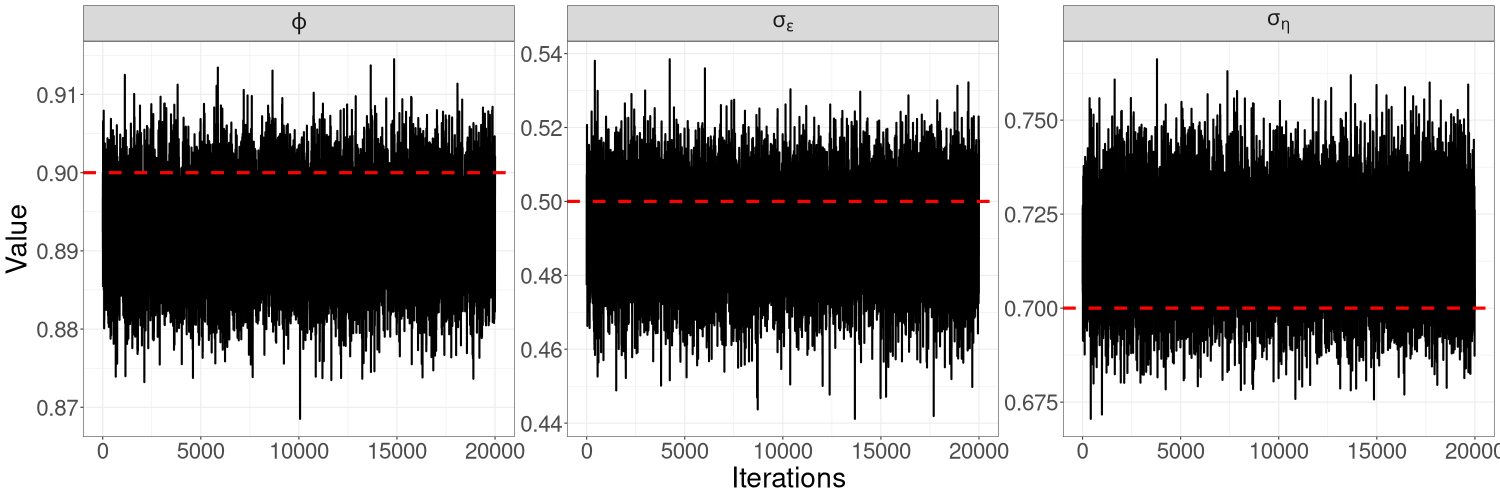
Figures 8(a) and 8(b) in Section S5 of the online supplement show the trace plots for each parameter obtained from HMC-exact and HMC-Whittle. Trace plots from both methods show good mixing for all three parameters but, for and in particular, HMC-Whittle has slightly better mixing than HMC-exact.
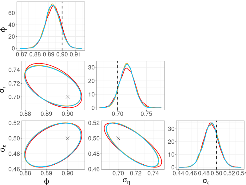
Figure 4 shows the marginal posterior distributions of the parameters, along with bivariate posterior distributions. The three methods yield very similar posterior distributions for all parameters. We also show in Section S3 of the online supplement that the posterior densities obtained from R-VGA-Whittle using block size are highly similar to those obtained without block updates. This suggests that block updates are useful for speeding up R-VGA-Whittle without compromising the accuracy of the approximate posterior densities.
| R-VGA-Whittle | HMC-Whittle | HMC-exact | ||
|---|---|---|---|---|
| Linear Gaussian | 10000 | 14 | 125 | 447 |
| SV (sim. data) | 10000 | 13 | 104 | 17005 |
| SV (real data) | 2649 | 13 | 25 | 3449 |
| 2D SV (sim. data) | 5000 | 121 | 14521 | 72170 |
| 2D SV (real data) | 2649 | 107 | 8890 | 74462 |
A comparison of the computing time between R-VGA-Whittle, HMC-Whittle and HMC-exact for this model can be found in Table 1. The table shows that R-VGA-Whittle is nearly 10 times faster than HMC-Whittle and more than 30 times faster than HMC-exact.
3.2 Univariate stochastic volatility model
SV models are a popular class of non-Gaussian financial time series models used for modelling the volatility of stock returns. An overview of SV models and traditional likelihood-based methods for parameter inference for use with these models can be found in Kim et al., (1998); an overview of MCMC-based inference for a univariate SV model can be found in Fearnhead, (2011).
In this section, we follow Fearnhead, (2011) and simulate observations from the following univariate SV model:
| (23) | ||||
| (24) | ||||
| (25) | ||||
| (26) |
We set the true parameters to , , and .
Following Ruiz, (1994), we apply a log-squared transformation,
| (27) |
where and , for . The terms are independent and identically distributed (iid) non-Gaussian terms with mean zero and variance (see Ruiz, (1994) for a derivation, which is reproduced in Section S2 of the online supplement for completeness).
Rearranging (27) yields the de-meaned series
| (28) |
Since , the parameter can be estimated using the sample mean:
As , once an estimate is obtained, can be estimated as
where , and is the digamma function (Abramowitz and Stegun,, 1968). As we show below, the estimate is not required for R-VGA-Whittle and HMC-Whittle as the Whittle likelihood does not depend on . However, appears in the likelihood used by HMC-exact. Since is not estimated by the Whittle-based methods, for comparison purposes we fix it to its estimate when using HMC-exact.
The remaining parameters to estimate are and . As with the linear Gaussian state space model, we work with the transformed parameters , where and , which are unconstrained. We fit the spectral density
| (29) |
to the log-squared, demeaned series , where
and is the Fourier transform of the covariance function of :
and is thus given by
| (30) |
The prior/initial variational distribution we use is
| (31) |
which leads to 95% probability intervals of for , and for . The interval for aligns closely with those used in similar studies of the stochastic volatility (SV) model. For example, Kim et al., (1998) employed the transformation with , resulting in a 95% probability interval for of . Additionally, Kim et al., (1998) utilized an inverse gamma prior for with shape and rate parameters of and , respectively, corresponding to a 95% probability interval for , which is comparable to the interval implied by our chosen prior.
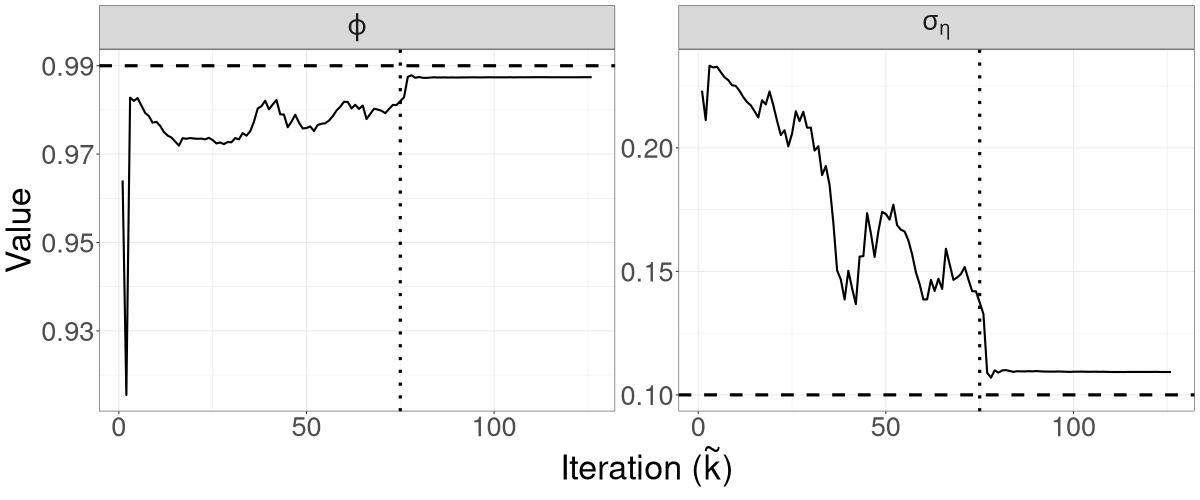
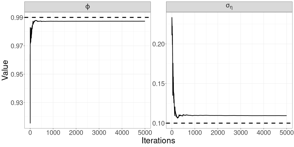
Figure 5 shows the trajectories of the R-VGA-Whittle variational means for all parameters. The 3dB cutoff point for this example is the 75th frequency, after which there are 50 blocks, for a total of 125 updates. Similar to the case of the LGSS model in Section 3.1, the variational mean of is close to the true value from the early stages of the algorithm, while that of requires more iterations to achieve convergence.
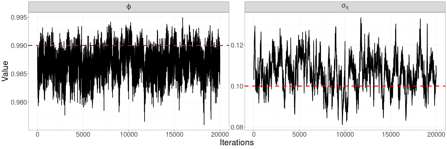
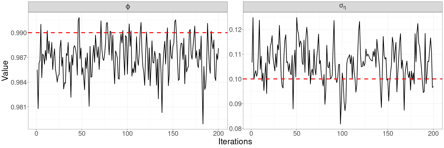
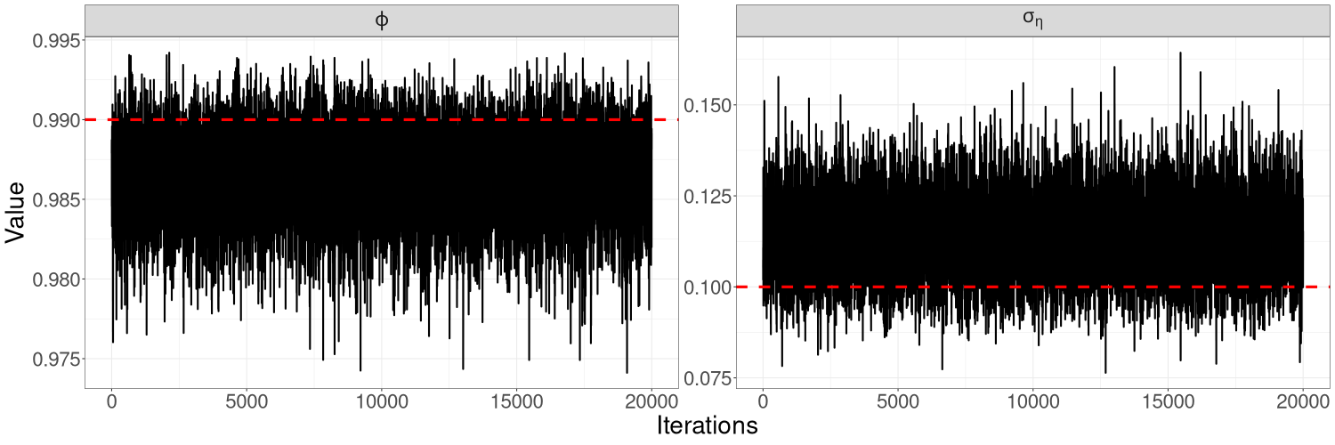
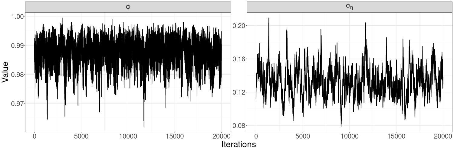
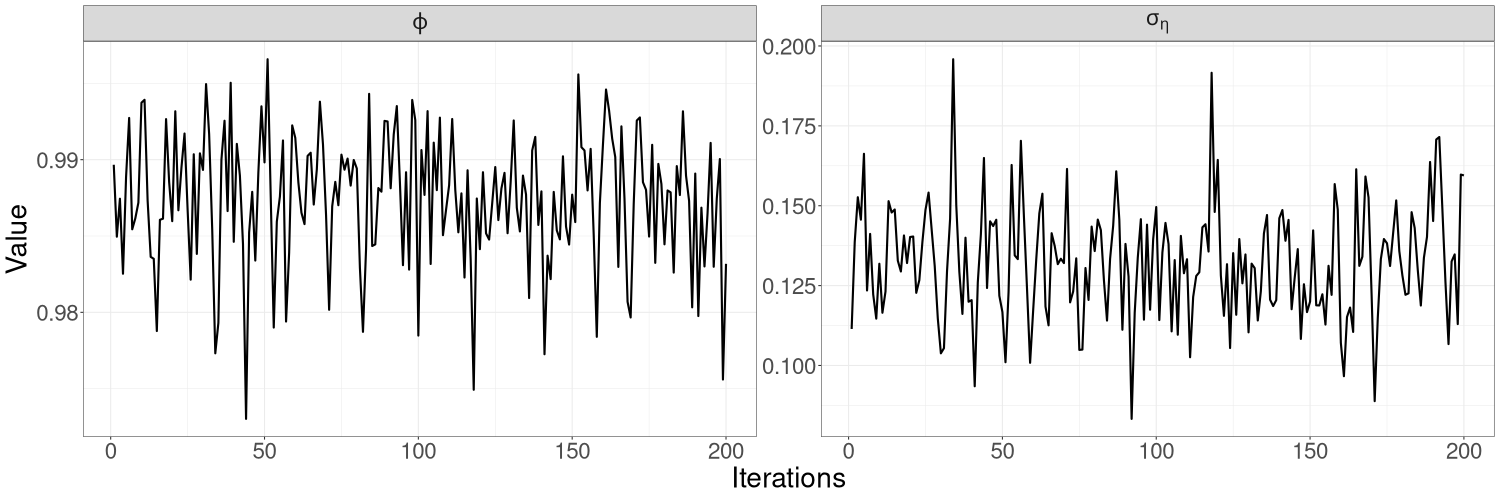
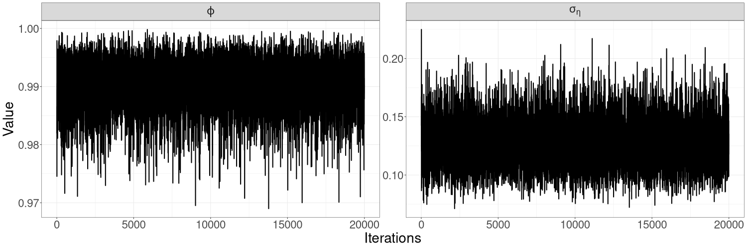
Figures 9(a) – 9(c) in Section S5 of the online supplement show the HMC-exact and HMC-Whittle trace plots. For this example, HMC-exact produces posterior samples with a much higher correlation than HMC-Whittle, particularly for the variance parameter . This is because HMC-Whittle only targets the posterior density of the parameters, while HMC-exact targets the joint posterior density of the states and parameters, which are high dimensional. We thin the posterior samples from HMC-exact by a factor of 100 for the remaining samples to be treated as uncorrelated draws from the posterior distribution.
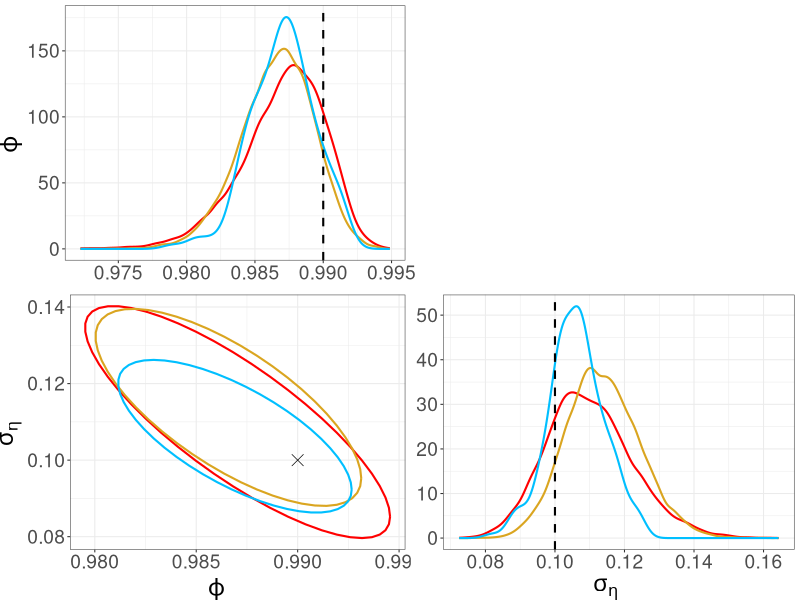
We compare the posterior densities from R-VGA-Whittle, HMC-Whittle, and HMC-exact in Figure 6. The posterior densities from R-VGA-Whittle and HMC-Whittle are very similar, while the posterior densities from HMC-exact are slightly narrower. Table 1 shows that R-VGA-Whittle is 8 times faster than HMC-Whittle, and more than 1000 times faster than HMC-exact in this example.
3.3 Bivariate SV model
We now consider the following bivariate extension of the SV model in Section 3.2 and simulate observations as follows:
| (32) | ||||
| (33) | ||||
| (34) |
where , , , and is the identity matrix. The covariance matrix is the solution to the equation , where is the vectorisation operator and denotes the Kronecker product of two matrices. We let be a diagonal matrix but let have off-diagonal entries so that there is dependence between the two series. We set these matrices to
| (35) |
As with the univariate model, we take a log-squared transformation of (32) to find
| (36) |
where
The terms and are iid non-Gaussian uncorrelated terms, each with mean zero and variance . We express (36) as
and use the sample means
as estimates of and , respectively. The parameters in this model are and . To estimate these parameters, we fit the following spectral density to :
where is the spectral density matrix of the VAR(1) process ,
| (37) |
with denoting the inverse of the conjugate transpose of the matrix , and is the spectral density of (following a similar derivation as that for the univariate SV model in Equation (30)).
We parameterise , , where is the lower Cholesky factor of , and the diagonal elements of as . The vector of transformed parameters is .
The initial/prior distribution we use is
| (38) |
For and , this prior leads to 95% probability intervals of . For , , and , the 95% probability intervals are , , and , respectively.
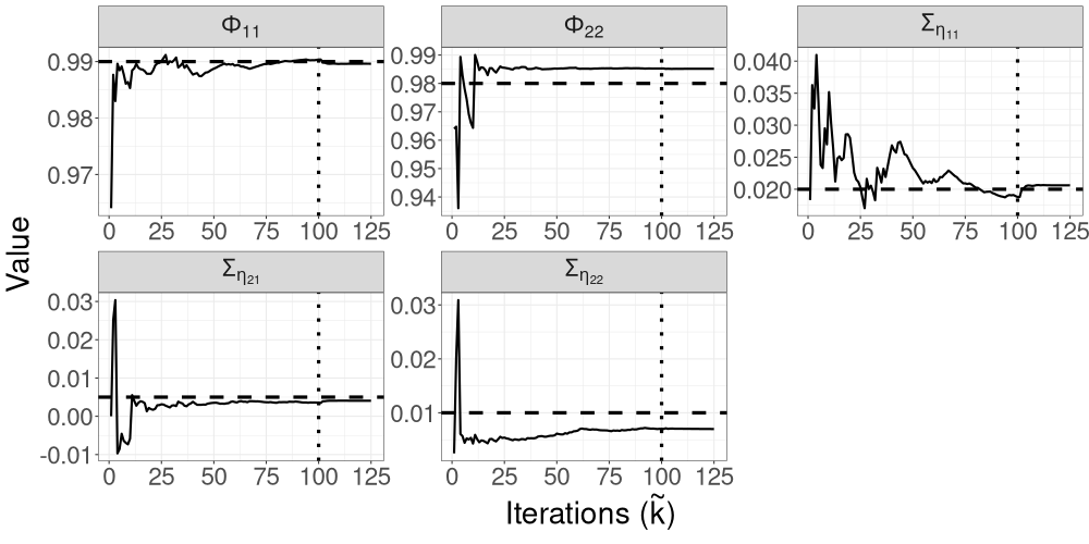
Figure 7 shows the trajectories of the R-VGA-Whittle variational means for all parameters in this model. For most parameters, the trajectories quickly move towards the true value within the first 10 to 20 updates, with only small adjustments afterwards. The only exception is for parameter , which exhibits more gradual changes before settling close to the true value in the last 25 iterations; this is somewhat expected since this parameter corresponds to a high-frequency signal component. R-VGA-Whittle slightly overestimated and underestimated .
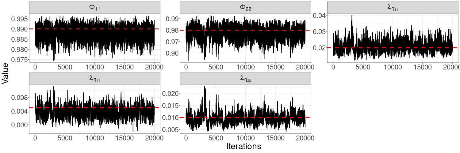
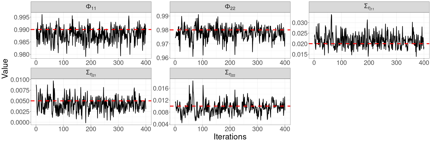
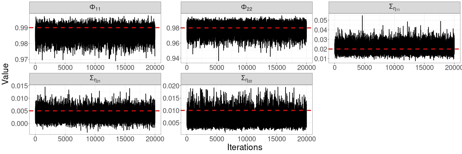
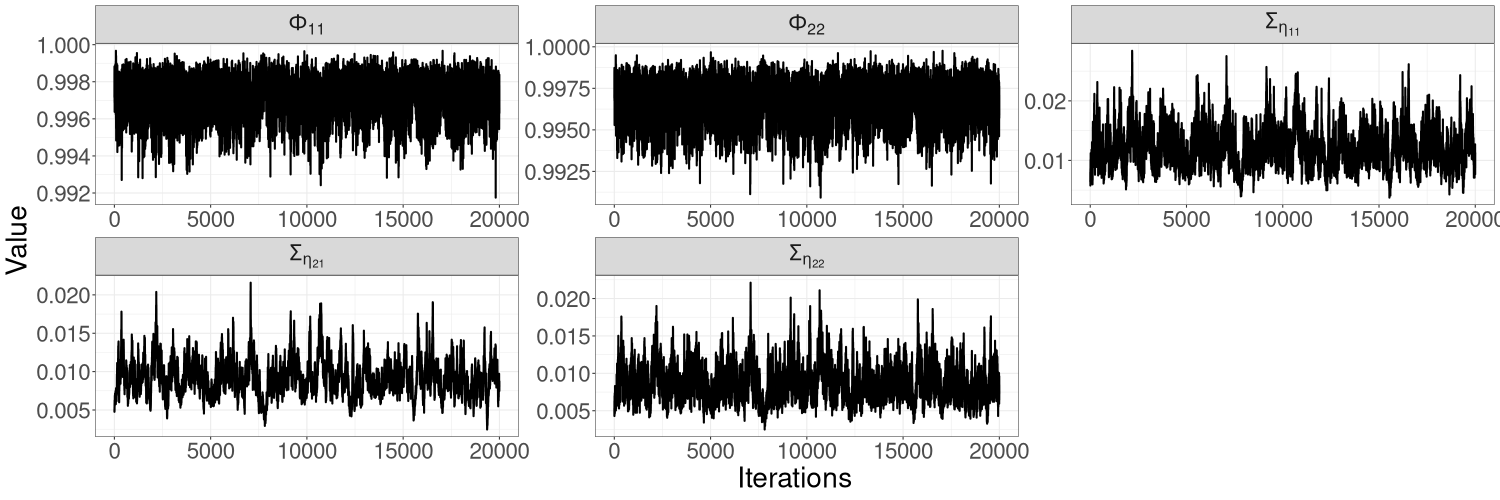
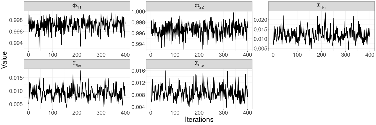
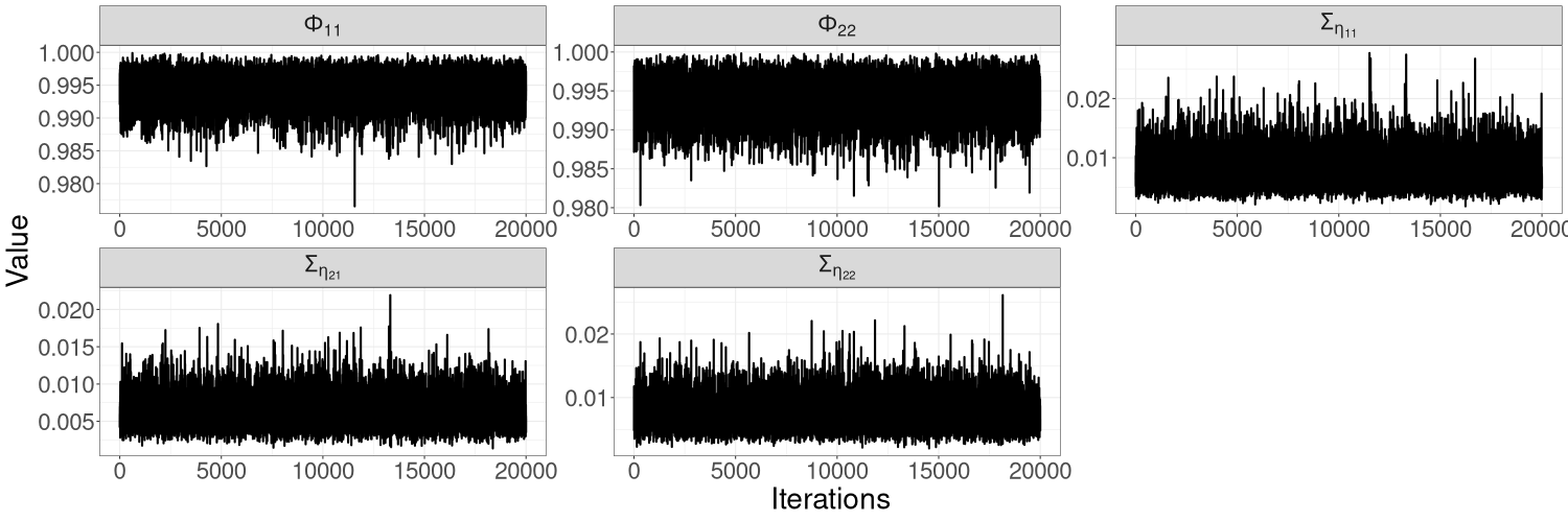
Figures 10(a)–10(c) in Section S5 of the online supplement show the HMC-exact and HMC-Whittle trace plots for this model. HMC-exact samples are highly correlated, especially those of . We find that it is necessary to thin the HMC-exact samples by a factor of 50 for the samples to be considered uncorrelated draws from the posterior distribution. In contrast, HMC-Whittle produces well-mixed posterior samples. Section S5 of the online supplement also shows that the effective sample sizes from HMC-Whittle are much higher than those from HMC-exact for all parameters.
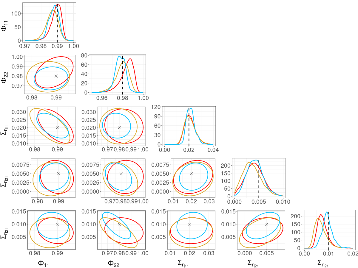
We compare the posterior densities from R-VGA-Whittle, HMC-Whittle, and HMC-exact in Figure 8. In this example, we observe broad agreement between the three methods, though the posterior densities from R-VGA-Whittle and HMC-Whittle are wider than those from HMC-exact. The posterior density of from R-VGA-Whittle puts more probability on values close to one than those from the other two methods, while the posterior density of from both R-VGA-Whittle and HMC-Whittle appear slightly shifted towards zero compared to that from HMC-exact. As shown in Table 1, R-VGA-Whittle is nearly 600 times faster than HMC-exact, and over 100 times faster than HMC-Whittle in this example.
3.4 Real univariate and bivariate examples
We apply R-VGA-Whittle to estimate parameters in univariate and bivariate stochastic volatility models from real data. We first apply it to daily JPY-EUR exchange rate data (Kastner et al.,, 2017) from April 1st, 2005 to August 6th, 2015, which consists of observations. Typically, the data used in SV models are de-meaned log-returns, which are computed from the raw exchange rate values as:
where is the exchange rate on day , and is the log-return on day . We fit the model (23)–(26) to this time series of de-meaned log-returns with , and use the initial variational distribution specified in (31).
The HMC-exact trace plots in Figures 11(a) of the online supplement show that posterior samples of are relatively well-mixed, but that the posterior samples of are highly correlated. We find it necessary to thin these samples by a factor of 100 in order for them to be considered uncorrelated. In contrast, HMC-Whittle produces well-mixed posterior samples, so that no thinning is needed.
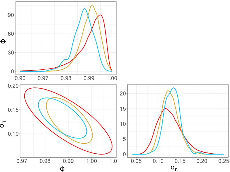
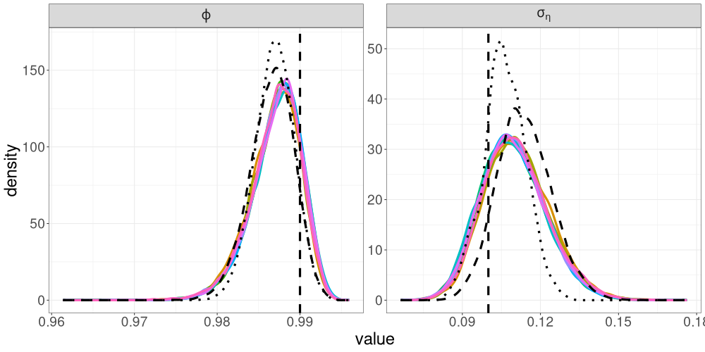
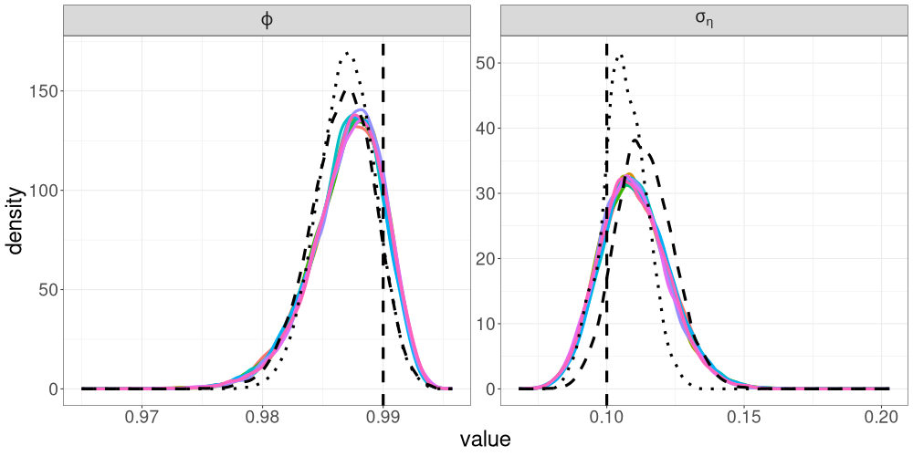
We compare the posterior densities from R-VGA-Whittle, HMC-Whittle and HMC-exact in Figure 9. The posterior densities obtained from R-VGA-Whittle are similar, but slightly wider than those obtained from HMC-Whittle and HMC-exact.
We also apply R-VGA-Whittle to a bivariate time series of daily GBP-EUR and USD-EUR exchange rates (Kastner et al.,, 2017) from April 1st, 2005, to August 6th, 2015, which consists of observations per exchange rate. We compute the de-meaned log-returns for both series and then fit the model (32)–(34) to these log-returns. The prior distribution we use is specified in (38).
Figures 12(a)–12(c) in Section S5 of the online supplement show the HMC-exact and HMC-Whittle trace plots for the bivariate SV model with exchange rate data. Similar to the simulation study, we find that HMC-exact samples are highly correlated; samples of parameters in tend to be less correlated than samples of parameters in . We thin the HMC-exact samples by a factor of 50 so that the remaining samples can be treated as uncorrelated. Posterior samples from HMC-Whittle have low correlation and are mixed well for all parameters, so no thinning is necessary.
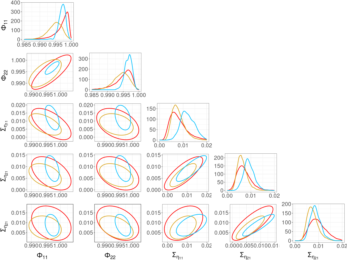
We compare the posterior densities from R-VGA-Whittle, HMC-Whittle, and HMC-exact in Figure 10. The marginal posterior densities from R-VGA-Whittle and HMC-Whittle are similar, but noticeably wider than the posterior densities from HMC-exact. Nevertheless, there is a substantial overlap between the posterior densities from all three methods.
Table 1 shows that R-VGA-Whittle is twice as fast as HMC-Whittle in the univariate case, and more than 80 times faster than HMC-Whittle in the bivariate case. R-VGA-Whittle is significantly faster than HMC-exact, with approximately a 260-fold speedup in the univariate case and a 700-fold speedup in the bivariate cases.
4 Conclusion
We develop a novel sequential variational Bayes algorithm that uses the Whittle likelihood, called R-VGA-Whittle, for parameter inference in linear non-Gaussian state space models. The Whittle likelihood is a frequency-domain approximation of the exact likelihood. It is available in closed form and its log can be expressed as a sum of individual log-likelihood frequency components. At each iteration, R-VGA-Whittle sequentially updates the variational parameters by processing one frequency or a block of frequencies at a time. We also demonstrate the use of the Whittle likelihood in HMC (HMC-Whittle), and compare the parameter estimates from R-VGA-Whittle and HMC-Whittle to those of HMC with the exact likelihood (HMC-exact). We show that the posterior densities from the three methods are generally similar, though posterior densities from R-VGA-Whittle and HMC-Whittle tend to be wider compared to those from HMC-exact. As HMC-Whittle only targets the parameters and not the states, it tends to produce posterior samples of the parameters that are less correlated than those from HMC-exact. We also show that R-VGA-Whittle and HMC-Whittle are much more computationally efficient than HMC-exact. R-VGA-Whittle is particularly efficient when dealing with bivariate time series, where it can be up to two orders of magnitude faster than HMC-Whittle and three orders of magnitude faster than HMC-exact.
There are several avenues for future research. First, R-VGA-Whittle assumes a Gaussian variational distribution, so future work could attempt to extend this framework to more flexible variational distributions for approximating skewed or multimodal posterior distributions. Second, some tuning parameters of R-VGA-Whittle (such as the number of damping observations and number of damping steps) are currently user-defined, so an adaptive tuning scheme could be developed to select these parameters. Third, as the Whittle likelihood is known to produce biased parameter estimates for finite sample sizes, using R-VGA-Whittle with the debiased Whittle likelihood of Sykulski et al., (2019) may improve parameter estimates.
Acknowledgements
This work was supported by ARC SRIEAS Grant SR200100005 Securing Antarctica’s Environmental Future. Andrew Zammit-Mangion’s research was also supported by ARC Discovery Early Career Research Award DE180100203.
References
- Abadi et al., (2015) Abadi, M., Agarwal, A., Barham, P., Brevdo, E., Chen, Z., Citro, C., Corrado, G. S., Davis, A., Dean, J., Devin, M., Ghemawat, S., Goodfellow, I., Harp, A., Irving, G., Isard, M., Jia, Y., Jozefowicz, R., Kaiser, L., Kudlur, M., Levenberg, J., Mané, D., Monga, R., Moore, S., Murray, D., Olah, C., Schuster, M., Shlens, J., Steiner, B., Sutskever, I., Talwar, K., Tucker, P., Vanhoucke, V., Vasudevan, V., Viégas, F., Vinyals, O., Warden, P., Wattenberg, M., Wicke, M., Yu, Y., and Zheng, X. (2015). TensorFlow: Large-scale machine learning on heterogeneous systems. Software available from tensorflow.org.
- Abadir et al., (2007) Abadir, K. M., Distaso, W., and Giraitis, L. (2007). Nonstationarity-extended local Whittle estimation. Journal of Econometrics, 141(2):1353–1384.
- Abramowitz and Stegun, (1968) Abramowitz, M. and Stegun, I. (1968). Handbook of Mathematical Functions with Formulas, Graphs, and Mathematical Tables. U.S. Government Printing Office, Washington, D. C.
- Andrieu and Roberts, (2009) Andrieu, C. and Roberts, G. O. (2009). The pseudo-marginal approach for efficient Monte Carlo computations. The Annals of Statistics, 37(2):697–725.
- Beal, (2003) Beal, M. J. (2003). Variational algorithms for approximate Bayesian inference. PhD thesis, University College London, UK.
- Blei et al., (2017) Blei, D. M., Kucukelbir, A., and McAuliffe, J. D. (2017). Variational inference: A review for statisticians. Journal of the American Statistical Association, 112(518):859–877.
- Bonnet, (1964) Bonnet, G. (1964). Transformations des signaux aléatoires a travers les systemes non linéaires sans mémoire. Annales des Télécommunications, 19:203–220.
- Brillinger, (2001) Brillinger, D. R. (2001). Time Series: Data Analysis and Theory. Society for Industrial and Applied Mathematics, Philadelphia, PA.
- Campbell et al., (2021) Campbell, A., Shi, Y., Rainforth, T., and Doucet, A. (2021). Online variational filtering and parameter learning. Advances in Neural Information Processing Systems, 34:18633–18645.
- Chan and Strachan, (2023) Chan, J. C. and Strachan, R. W. (2023). Bayesian state space models in macroeconometrics. Journal of Economic Surveys, 37(1):58–75.
- Cooley and Tukey, (1965) Cooley, J. W. and Tukey, J. W. (1965). An algorithm for the machine calculation of complex Fourier series. Mathematics of Computation, 19(90):297–301.
- Doucet and Shephard, (2012) Doucet, A. and Shephard, N. G. (2012). Robust inference on parameters via particle filters and sandwich covariance matrices. Discussion paper series, Department of Economics, University of Oxford, UK.
- Duane et al., (1987) Duane, S., Kennedy, A. D., Pendleton, B. J., and Roweth, D. (1987). Hybrid Monte Carlo. Physics Letters B, 195(2):216–222.
- Dukic et al., (2012) Dukic, V., Lopes, H. F., and Polson, N. G. (2012). Tracking epidemics with Google flu trends data and a state-space SEIR model. Journal of the American Statistical Association, 107(500):1410–1426.
- Dzhaparidze and Yaglom, (1983) Dzhaparidze, K. and Yaglom, A. (1983). Spectrum parameter estimation in time series analysis. In Krishnaiah, P. R., editor, Developments in Statistics, pages 1–96. Academic Press, New York, NY.
- Fearnhead, (2011) Fearnhead, P. (2011). MCMC for state-space models. In Brooks, S., Gelman, A., Jones, G. J., and Meng, X.-L., editors, Handbook of Markov Chain Monte Carlo, pages 513–530. CRC Press, Boca Raton, FL.
- Frazier et al., (2023) Frazier, D. T., Loaiza-Maya, R., and Martin, G. M. (2023). Variational Bayes in state space models: Inferential and predictive accuracy. Journal of Computational and Graphical Statistics, 32(3):793–804.
- Fuentes, (2007) Fuentes, M. (2007). Approximate likelihood for large irregularly spaced spatial data. Journal of the American Statistical Association, 102(477):321–331.
- Gabry et al., (2024) Gabry, J., Češnovar, R., and Johnson, A. (2024). Getting started with CmdStanR.
- Gibson and Ninness, (2005) Gibson, S. and Ninness, B. (2005). Robust maximum-likelihood estimation of multivariable dynamic systems. Automatica, 41(10):1667–1682.
- Giraitis et al., (2012) Giraitis, L., Koul, H. L., and Surgailis, D. (2012). Large Sample Inference for Long Memory Processes. Imperial College Press, London, UK.
- Giraitis and Robinson, (2001) Giraitis, L. and Robinson, P. M. (2001). Whittle estimation of ARCH models. Econometric Theory, 17(3):608–631.
- Gordon et al., (1993) Gordon, N. J., Salmond, D. J., and Smith, A. F. (1993). Novel approach to nonlinear/non-Gaussian Bayesian state estimation. IEE Proceedings F, 140(2):107–113.
- Gunawan et al., (2021) Gunawan, D., Kohn, R., and Nott, D. (2021). Variational Bayes approximation of factor stochastic volatility models. International Journal of Forecasting, 37(4):1355–1375.
- Gunawan et al., (2024) Gunawan, D., Kohn, R., and Nott, D. (2024). Flexible variational Bayes based on a copula of a mixture. Journal of Computational and Graphical Statistics, 33(2):665–680.
- Harvey, (1990) Harvey, A. C. (1990). Forecasting, Structural Time Series Models and the Kalman Filter. Cambridge University Press, Cambridge, UK.
- Hoffman and Gelman, (2014) Hoffman, M. D. and Gelman, A. (2014). The No-U-Turn sampler: adaptively setting path lengths in Hamiltonian Monte Carlo. Journal of Machine Learning Research, 15(1):1593–1623.
- Hurvich and Chen, (2000) Hurvich, C. M. and Chen, W. W. (2000). An efficient taper for potentially overdifferenced long-memory time series. Journal of Time Series Analysis, 21(2):155–180.
- Kantas et al., (2009) Kantas, N., Doucet, A., Singh, S. S., and Maciejowski, J. M. (2009). An overview of sequential monte carlo methods for parameter estimation in general state-space models. IFAC Proceedings Volumes, 42(10):774–785.
- Kastner et al., (2017) Kastner, G., Frühwirth-Schnatter, S., and Lopes, H. F. (2017). Efficient Bayesian inference for multivariate factor stochastic volatility models. Journal of Computational and Graphical Statistics, 26(4):905–917.
- Kim et al., (1998) Kim, S., Shephard, N., and Chib, S. (1998). Stochastic volatility: likelihood inference and comparison with ARCH models. The Review of Economic Studies, 65(3):361–393.
- Lambert et al., (2022) Lambert, M., Bonnabel, S., and Bach, F. (2022). The recursive variational Gaussian approximation (R-VGA). Statistics and Computing, 32(10).
- Laplace, (1986) Laplace, P. S. (1986). Memoir on the probability of the causes of events. Statistical Science, 1(3):364–378.
- Loaiza-Maya et al., (2022) Loaiza-Maya, R., Smith, M. S., Nott, D. J., and Danaher, P. J. (2022). Fast and accurate variational inference for models with many latent variables. Journal of Econometrics, 230(2):339–362.
- Mangion et al., (2011) Mangion, A. Z., Yuan, K., Kadirkamanathan, V., Niranjan, M., and Sanguinetti, G. (2011). Online variational inference for state-space models with point-process observations. Neural Computation, 23(8):1967–1999.
- Matsuda and Yajima, (2009) Matsuda, Y. and Yajima, Y. (2009). Fourier analysis of irregularly spaced data on . Journal of the Royal Statistical Society Series B, 71(1):191–217.
- Meyer et al., (2003) Meyer, R., Fournier, D. A., and Berg, A. (2003). Stochastic volatility: Bayesian computation using automatic differentiation and the extended Kalman filter. The Econometrics Journal, 6(2):408–420.
- Neal, (2011) Neal, R. (2011). MCMC using Hamiltonian dynamics. In Brooks, S., Gelman, A., Jones, G. J., and Meng, X.-L., editors, Handbook of Markov Chain Monte Carlo. CRC Press, Boca Raton, FL.
- Nemeth et al., (2016) Nemeth, C., Fearnhead, P., and Mihaylova, L. (2016). Particle approximations of the score and observed information matrix for parameter estimation in state–space models with linear computational cost. Journal of Computational and Graphical Statistics, 25(4):1138–1157.
- Percival and Walden, (1993) Percival, D. B. and Walden, A. T. (1993). Spectral Analysis for Physical Applications. Cambridge University Press, Cambridge, UK.
- Price, (1958) Price, R. (1958). A useful theorem for nonlinear devices having Gaussian inputs. IRE Transactions on Information Theory, 4(2):69–72.
- Robinson, (1995) Robinson, P. M. (1995). Gaussian semiparametric estimation of long range dependence. The Annals of Statistics, 23(5):1630–1661.
- Ruiz, (1994) Ruiz, E. (1994). Quasi-maximum likelihood estimation of stochastic volatility models. Journal of Econometrics, 63(1):289–306.
- Salomone et al., (2020) Salomone, R., Quiroz, M., Kohn, R., Villani, M., and Tran, M.-N. (2020). Spectral subsampling MCMC for stationary time series. In Proceedings of the 37th International Conference on Machine Learning, pages 8449–8458. PMLR.
- (45) Shao, X. and Wu, W. B. (2007a). Asymptotic spectral theory for nonlinear time series. The Annals of Statistics, 35(4):1773–1801.
- (46) Shao, X. and Wu, W. B. (2007b). Local Whittle estimation of fractional integration for nonlinear processes. Econometric Theory, 23(5):899–929.
- She et al., (2022) She, R., Mi, Z., and Ling, S. (2022). Whittle parameter estimation for vector ARMA models with heavy-tailed noises. Journal of Statistical Planning and Inference, 219:216–230.
- Sykulski et al., (2019) Sykulski, A. M., Olhede, S. C., Guillaumin, A. P., Lilly, J. M., and Early, J. J. (2019). The debiased Whittle likelihood. Biometrika, 106(2):251–266.
- Tan and Nott, (2018) Tan, L. S. and Nott, D. J. (2018). Gaussian variational approximation with sparse precision matrices. Statistics and Computing, 28:259–275.
- Tomasetti et al., (2022) Tomasetti, N., Forbes, C., and Panagiotelis, A. (2022). Updating variational Bayes: Fast sequential posterior inference. Statistics and Computing, 32(4).
- Tran et al., (2017) Tran, M.-N., Nott, D. J., and Kohn, R. (2017). Variational Bayes with intractable likelihood. Journal of Computational and Graphical Statistics, 26(4):873–882.
- Villani et al., (2022) Villani, M., Quiroz, M., Kohn, R., and Salomone, R. (2022). Spectral subsampling MCMC for stationary multivariate time series with applications to vector ARTFIMA processes. Econometrics and Statistics.
- Vu et al., (2024) Vu, B. A., Gunawan, D., and Zammit-Mangion, A. (2024). R-VGAL: a sequential variational Bayes algorithm for generalised linear mixed models. Statistics and Computing, 34(110).
- Welch, (1967) Welch, P. (1967). The use of fast Fourier transform for the estimation of power spectra: A method based on time averaging over short, modified periodograms. IEEE Transactions on Audio and Electroacoustics, 15(2):70–73.
- Whittle, (1953) Whittle, P. (1953). Estimation and information in stationary time series. Arkiv för Matematik, 2(5):423–434.
- Zammit Mangion et al., (2011) Zammit Mangion, A., Sanguinetti, G., and Kadirkamanathan, V. (2011). A variational approach for the online dual estimation of spatiotemporal systems governed by the IDE. IFAC Proceedings Volumes, 44(1):3204–3209. 18th IFAC World Congress.
- Zammit-Mangion et al., (2012) Zammit-Mangion, A., Sanguinetti, G., and Kadirkamanathan, V. (2012). Variational estimation in spatiotemporal systems from continuous and point-process observations. IEEE Transactions on Signal Processing, 60(7):3449–3459.
S1 The R-VGA algorithm
In this section, we provide a sketch of the derivations for the R-VGA algorithm of Lambert et al., (2022), which serves as the basis for our R-VGA-Whittle algorithm.
The R-VGA algorithm of Lambert et al., (2022) requires iid observations, denoted by , and approximates the posterior distribution with a Gaussian distribution . By assumption of conditional independence between observations given the parameters , the KL divergence between the variational distribution and the posterior distribution can be expressed as
In a sequential VB framework, the posterior distribution after incorporating the first observations, , is approximated by the variational distribution to give
| (S1) |
As the last two terms on the right hand side of (S1) do not depend on , the KL-minimisation problem is equivalent to solving
| (S2) |
Differentiating the expectation in (S2) with respect to and , setting the derivatives to zero, and rearranging the resulting equations, yields the following recursive updates for the variational mean and precision matrix :
| (S3) | ||||
| (S4) |
Then, using Bonnet’s Theorem (Bonnet,, 1964) on (S3) and Price’s Theorem (Price,, 1958) on (S4), we rewrite the gradient terms as
| (S5) | ||||
| (S6) |
Thus the updates (S3) and (S4) become
| (S7) | ||||
| (S8) |
These updates are implicit as they require the evaluation of expectations with respect to . Under the assumption that is close to , Lambert et al., (2022) propose replacing with in (S7) and (S8), and replacing with on the right hand side of (S7), to yield an explicit scheme
| (S9) | ||||
| (S10) |
Equations (S9) and (S10) form the so-called R-VGA algorithm of Lambert et al., (2022).
S2 Additional details on the SV model
In this section, we follow Ruiz, (1994) and show that the terms in the log-squared transformation (27) in the main paper have mean zero and variance .
Since , we have , that is, is gamma distributed with shape and scale parameters equal to and , respectively. Therefore, has mean , where denotes the digamma function (the first derivative of the logarithm of the gamma function), and variance , where is the trigamma function (the second derivative of the logarithm of the gamma function; see, e.g., Abramowitz and Stegun, (1968)). Thus
and
S3 Experiments involving different blocking strategies
In this section, we discuss the tuning parameters in Algorithm 3: the choice of block length and the number of frequencies to be processed individually before blocking, . We base our discussion on inspection of the periodogram.
Recall that the periodogram is an estimate of the spectral density and can be viewed as a measure of the relative contributions of the frequencies to the total variance of the process (Percival and Walden,, 1993). For example, Figure S1 shows the periodograms for the linear Gaussian SSM in Section 3.1 and the univariate SV model in Section 3.2. This figure shows that in general, power decreases as frequency increases. Frequencies that carry less power tend to have less effect on the trajectory of the variational mean; see, for example, the trajectories of the parameters of the linear Gaussian model in Figure S2. The trajectory of moves towards the true parameter value within the first few frequencies, with only minor adjustments afterwards. The trajectories for and behave in a similar manner, but with more gradual changes. This behaviour can also be observed in Figure S3, in which the trajectories of both parameters in the univariate SV model exhibit large changes in the first few iterations, then stabilise afterwards. Higher frequencies that have little effect on the variational mean can thus be processed together in “blocks”. The R-VGA-Whittle updates can then be made based on the Whittle log-likelihood for a “block” of frequencies, which we compute as the sum of the individual log-likelihood contribution evaluated at each frequency within that block.
It is important to choose an appropriate point to start blocking, as well as an appropriate length for each block of frequencies. To determine the frequency at which to begin blocking, we borrow a concept from physics and electrical engineering called the 3dB frequency cutoff, which is the frequency on the power spectrum at which the power drops to approximately half the maximum power of the spectrum. The value 3 comes from the fact that, on the decibel scale, a drop from a power level to another level results in a drop of 3 decibels. The change in decibels is calculated as
We employ a similar idea here, where we define the “cutoff” frequency as the frequency at which the power drops to half of the maximum power in a smoothed version of the periodogram. Specifically, we seek the frequency such that , where is the periodogram smoothed using Welch’s method (Welch,, 1967). Briefly, Welch’s method works by dividing the frequencies into equal segments, computing the periodogram for each segment, and then averaging over these segments to obtain a smoother periodogram with lower variance. We also experiment with other cutoffs, such as the frequencies at which the power are one-fifth and one-tenth of the maximum power in the smoothed periodogram, which correspond to a drop of approximately 7dB and 10dB, respectively. We mark these cutoff frequencies in Figure S1.
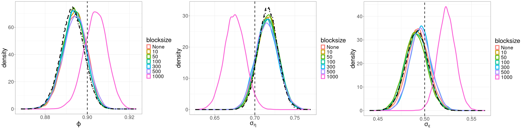
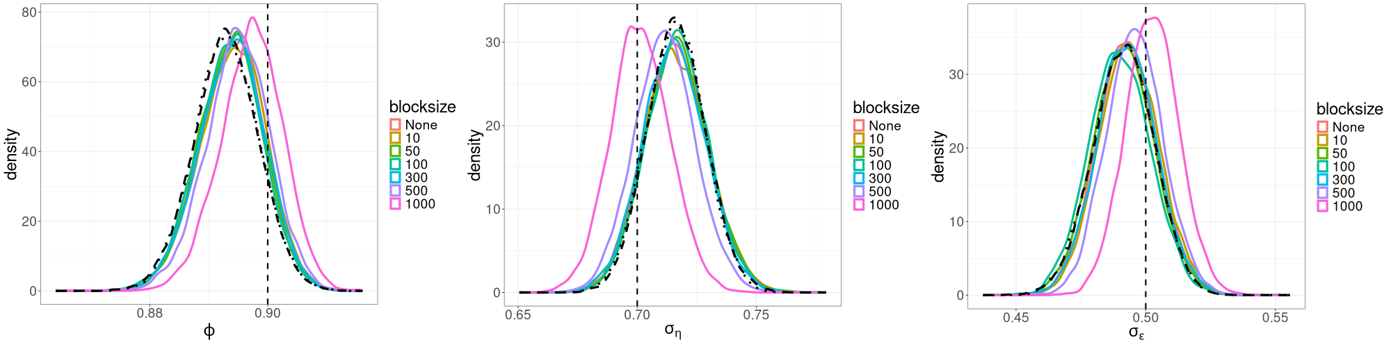
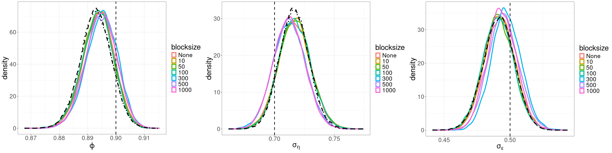
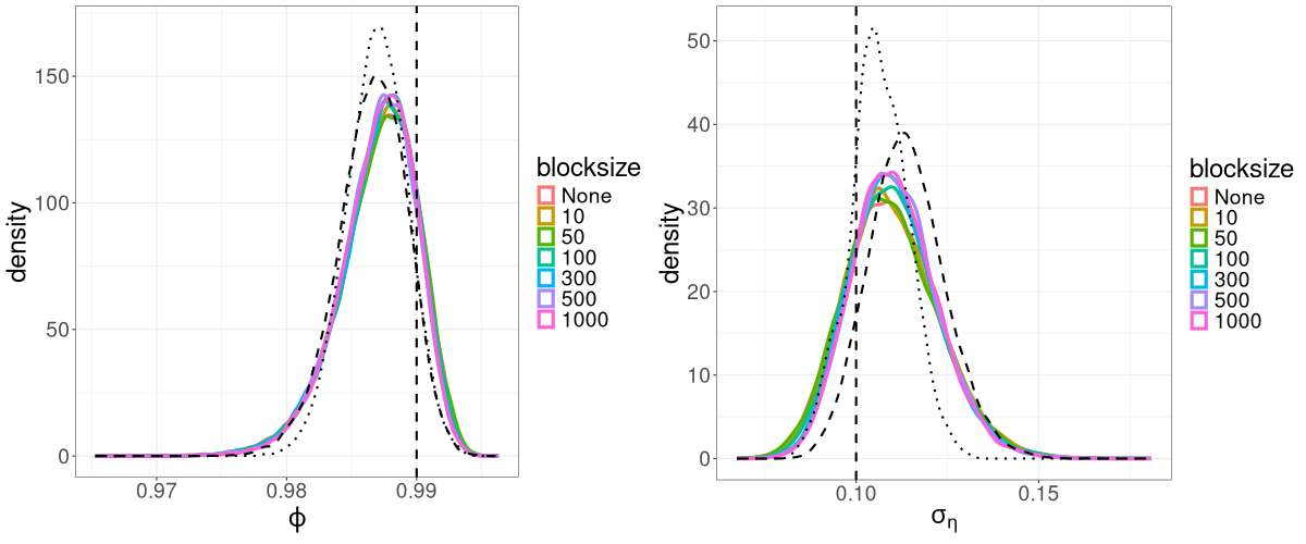
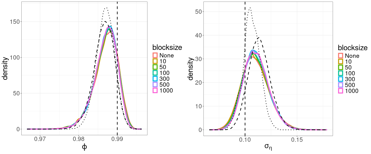
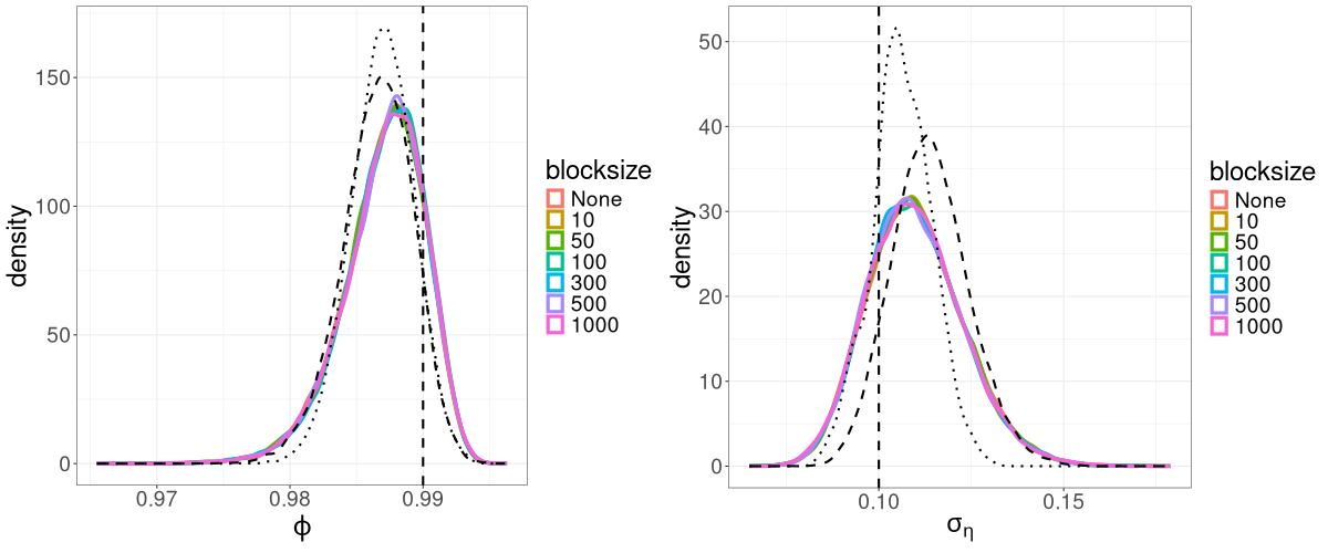
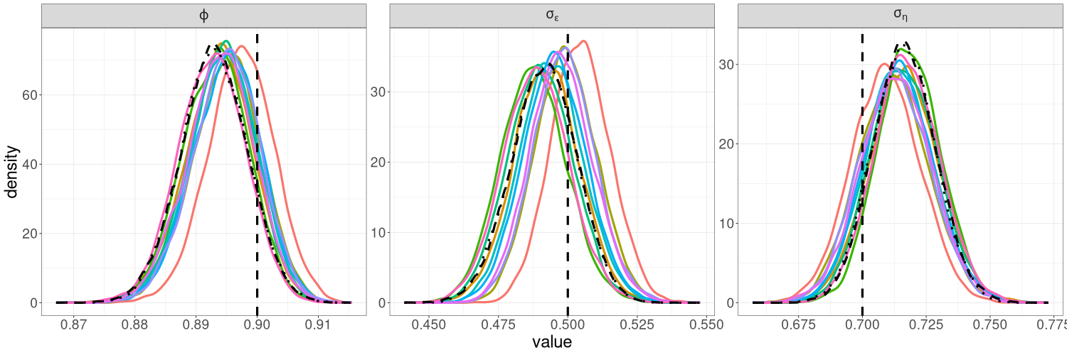
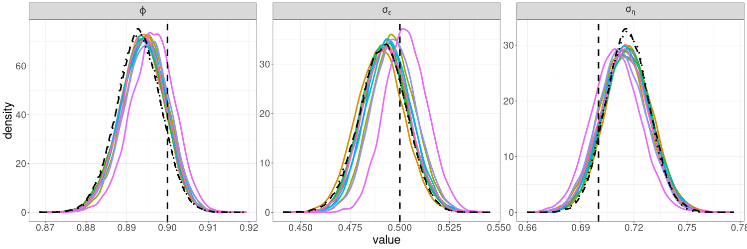
Using each of the 3dB, 7dB and 10dB cutoffs, we run R-VGA-Whittle with no blocking, and then with varying block sizes (, and frequencies), and examine the posterior densities of the parameters under these different settings. For all runs, we keep the settings for other tuning parameters the same as in Section 3 and use Monte Carlo samples, , and damping steps. For the linear Gaussian SSM, we plot the R-VGA-Whittle posteriors for these different cutoffs and block sizes in Figures 4(a), 4(b) and 4(c). The corresponding plots for the univariate SV model are shown in Figures 5(a), 5(b), and 5(c). The plots for the bivariate SV model are similar to those from the univariate SV model and not shown.
We find that for the linear Gaussian SSM, block sizes of and below result in R-VGA-Whittle posterior densities that are very similar to each other, similar to the posterior densities obtained without blocking, and also similar to the posterior densities from HMC-Whittle and HMC-exact. For block sizes of and , the posterior densities of the parameters and begin to differ slightly compared to the posterior densities obtained without blocking. When the block size is , the posterior densities for all three parameters become noticeably biased, although this bias reduces when the frequency cutoff point increases, as expected. However, for the SV model, the R-VGA-Whittle posterior densities are highly similar for all block sizes. To achieve the best reduction in computing time while retaining estimation accuracy, we choose to begin blocking at the earliest cutoff point we consider in this experiment (3dB), with the block size set to 100.
S4 Variance of the R-VGA-Whittle posterior densities for various Monte Carlo sample sizes
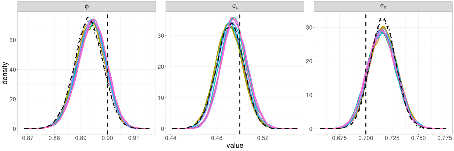
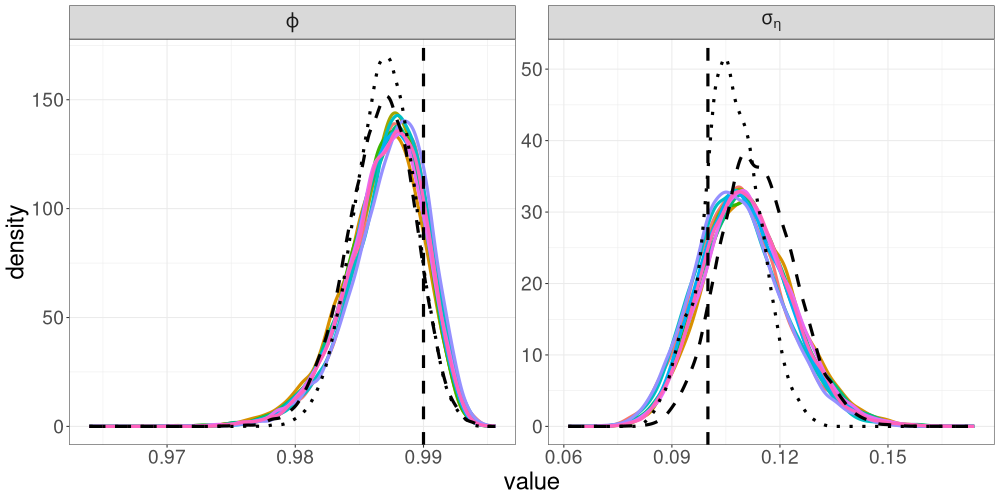
In this section, we study the robustness of R-VGA-Whittle posterior distributions to different values of , the Monte Carlo sample size used to approximate the expectations of the gradient and Hessian in Algorithm 2. We consider sample sizes and . We apply blocking as in Algorithm 3, and fix the block length to . We set for the linear Gaussian SSM, and for the univariate SV model, which corresponds to the 3dB cutoff point as discussed in Section S3.
Figures 6(a)–6(c) show the posterior densities of the parameters of the linear Gaussian SSM from 10 runs of R-VGA-Whittle with , , and , respectively, while Figures 7(a)–7(c) show the corresponding plots for the SV model. As the Monte Carlo sample size increases, the variance in the posterior densities across different runs decreases. When , the variance across different runs is significantly reduced, so we choose this as our Monte Carlo sample size for all examples in Section 3 of the main paper.
S5 Trace plots
This section shows the HMC-exact and HMC-Whittle trace plots and effective sample size (ESS) for the parameters in all the models we consider. Figure S8 shows trace plots for the linear Gaussian SSM, Figures S9 and S10 show trace plots for the univariate and bivariate SV models with simulated data, and Figures S11 and S12 show trace plots for the univariate and bivariate SV models with real data.
In general, we find that HMC-Whittle tends to produce posterior samples with much lower correlation than HMC-exact. For the same number of posterior samples, HMC-Whittle has higher ESS than HMC-exact, and the ESS of HMC-Whittle is high for all paramaters, while HMC-exact tends to produce higher ESS for the autoregressive parameters ( for univariate examples and for bivariate examples) than for the variance parameters ( and for the linear Gaussian model, for the univariate SV model, and for the bivariate SV model). This is because HMC-Whittle only targets the posterior density of the parameters, whereas HMC-exact targets the joint posterior density of the parameters and states, which are high dimensional. See Table S1 for the ESS corresponding to each parameter in our examples.
| Example | Parameter | ESS (HMC-exact) | ESS (HMC-Whittle) |
|---|---|---|---|
| Linear Gaussian | 2452.8033 | 8884.775 | |
| Linear Gaussian | 846.3039 | 7933.656 | |
| Linear Gaussian | 697.3547 | 8163.235 | |
| Univariate SV (sim. data) | 230.00751 | 6854.622 | |
| Univariate SV (sim. data) | 87.94789 | 6949.066 | |
| Bivariate SV (sim. data) | 814.3441 | 13064.54 | |
| Bivariate SV (sim. data) | 282.3187 | 12967.59 | |
| Bivariate SV (sim. data) | 346.6532 | 13382.68 | |
| Bivariate SV (sim. data) | 440.2904 | 16141.23 | |
| Bivariate SV (sim. data) | 138.6995 | 12034.28 | |
| Univariate SV (real data) | 304.6549 | 5920.983 | |
| Univariate SV (real data) | 118.8147 | 5980.517 | |
| Bivariate SV (real data) | 730.7380 | 9058.774 | |
| Bivariate SV (real data) | 796.0991 | 9242.738 | |
| Bivariate SV (real data) | 206.4234 | 11170.016 | |
| Bivariate SV (real data) | 161.9922 | 9989.325 | |
| Bivariate SV (real data) | 245.5852 | 11127.356 |