Recursively-Constrained Partially Observable Markov Decision Processes
Abstract
Many sequential decision problems involve optimizing one objective function while imposing constraints on other objectives. Constrained Partially Observable Markov Decision Processes (C-POMDP) model this case with transition uncertainty and partial observability. In this work, we first show that C-POMDPs violate the optimal substructure property over successive decision steps and thus may exhibit behaviors that are undesirable for some (e.g., safety critical) applications. Additionally, online re-planning in C-POMDPs is often ineffective due to the inconsistency resulting from this violation. To address these drawbacks, we introduce the Recursively-Constrained POMDP (RC-POMDP), which imposes additional history-dependent cost constraints on the C-POMDP. We show that, unlike C-POMDPs, RC-POMDPs always have deterministic optimal policies and that optimal policies obey Bellman’s principle of optimality. We also present a point-based dynamic programming algorithm for RC-POMDPs. Evaluations on benchmark problems demonstrate the efficacy of our algorithm and show that policies for RC-POMDPs produce more desirable behaviors than policies for C-POMDPs.
1 Introduction
Partially Observable Markov Decision Processes (POMDPs) are powerful models for sequential decision making due to their ability to account for transition uncertainty and partial observability. Their applications range from autonomous driving Pendleton et al. [2017] and robotics to geology Lauri et al. [2023], Wang et al. [2022], asset maintenance Papakonstantinou and Shinozuka [2014], and human-computer interaction Chen et al. [2020]. Constrained POMDPs (C-POMDPs) are extensions of POMDPs that impose a bound on expected cumulative costs while seeking policies that maximize expected total reward. C-POMDPs address the need to consider multiple objectives in applications such as autonomous rover that may have a navigation task as well as an energy usage budget, or human-AI dialogue systems with constraints on the length of dialogues. However, we observe that optimal policies computed for C-POMDPs exhibit pathological behavior in some problems, which can be opposed to the C-POMDP’s intended purpose.
Example 1 (Cave Navigation).
Consider a rover agent in a cave with two tunnels, A and B, which may have rocky terrains. Traversing tunnel A has a higher expected reward than traversing tunnel B. To model wheel damage, a cost of is given for traversing through rocky terrain, and otherwise. The agent has noisy observations (correct with a probability of ) of a tunnel’s terrain type, and hence, has to maintain a belief (probability distribution) over the terrain type in each tunnel. The task is to navigate to the end of a tunnel while ensuring that the expected total cost is below a threshold of . The agent has the initial belief of probability of rocks and probability of no rocks in tunnel , and probability of rocks and probability of no rocks in tunnel .
In this example, suppose the agent receives an observation that leads to an updated belief of probability that tunnel is rocky. Intuitively, the agent should avoid tunnel since the expected cost of navigating it is , which violates the cost constraint of . However, an optimal policy computed from a C-POMDP decides to go through the rocky region, violating the constraint and damaging the wheels. Such behavior is justified in the C-POMDP framework by declaring that, due to a low probability of observing that tunnel is rocky in the first place, the expected cost from the initial time step is still within the threshold, and so this policy is admissible. However, this pathological behavior is clearly unsuitable especially for some (e.g., safety-critical) applications.
In this paper, we first provide the key insight that the pathological behavior is caused by the violation of the optimal substructure property over successive decision steps, and hence violation of the standard form of Bellman’s Principle of Optimality (BPO). To mitigate the pathological behavior and preserve the optimal substructure property, we propose an extension of C-POMDPs through the addition of history-dependent cost constraints at each reachable belief, which we call Recursively-Constrained POMDPs (RC-POMDPs). We prove that deterministic policies are sufficient for optimality in RC-POMDPs and that RC-POMDPs satisfy BPO. These results suggest that RC-POMDPs are highly amenable to standard dynamic programming techniques, which is not true for C-POMDPs. RC-POMDPs provide a good balance between the BPO-violating expectation constraints of C-POMDPs and constraints on the worst-case outcome, which are overly conservative for POMDPs with inherent state uncertainty. Then, we present a point-based dynamic programming algorithm to approximately solve RC-POMDPs. Experimental evaluation shows that the pathological behavior is a prevalent phenomenon in C-POMDP policies, and that our algorithm for RC-POMDPs computes polices which obtain expected cumulative rewards competitive with C-POMDPs without exhibiting such behaviors.
In summary, this paper contributes (i) an analysis that C-POMDPs do not exhibit the optimal substructure property over successive decision steps and its consequences, (ii) the introduction of RC-POMDPs, a novel extension of C-POMDPs through the addition of history-dependent cost constraints, (iii) proofs that all RC-POMDPs have at least one deterministic optimal policy, satisfy BPO, and the Bellman operator has a unique fixed point under suitable initializations, (iv) a dynamic programming algorithm for RC-POMDPs, and (v) a series of illustrative benchmarks to demonstrate the advantages of RC-POMDPs.
Related Work
Several solution approaches exist for C-POMDPs with expectation constraints de Nijs et al. [2021]. These include offline Isom et al. [2008], Kim et al. [2011], Poupart et al. [2015], Walraven and Spaan [2018], Kalagarla et al. [2022], Wray and Czuprynski [2022] and online methods Lee et al. [2018], Jamgochian et al. [2023]. These works suffer from the unintuitive behavior discussed above. This paper shows that this behavior is rooted in the violation of optimal substructure by C-POMDPs and proposes a new problem formulation that obeys BPO.
BPO violation has also been discussed in fully-observable Constrained MDPs (C-MDPs) with state-action frequency and long-run average cost constraints Haviv [1996], Chong et al. [2012]. To overcome it, Haviv [1996] proposes an MDP formulation with sample path constraints. In C-POMDPs with expected cumulative costs, this BPO-violation problem remains unexplored. Additionally, adoption of the MDP solution of worst-case sample path constraints would be overly conservative for POMDPs, which are inherently characterized by state uncertainty. This paper fills that gap by studying the BPO of C-POMDPs and addressing it by imposing recursive expected cost constraints.
From the algorithmic perspective, the closest work to ours is the C-POMDP point-based value iteration (CPBVI) algorithm Kim et al. [2011]. Samples of admissible costs, defined by Piunovskiy and Mao [2000] for C-MDPs, are used with belief points as a heuristic to improve computational tractability of point-based value iteration for C-POMDPs. However, since CPBVI is designed for C-POMDPs, the synthesized policies by CPBVI may still exhibit pathological behavior. In this paper, we formalize the use of history-dependent expected cost constraints and provide a thorough analysis of it. We show that this problem formulation eliminates the pathological behavior of C-POMDPs.
2 Constrained POMDPs
POMDPs model sequential decision making problems under transition uncertainty and partial observability.
Definition 1 (POMDP).
A Partially Observable Markov Decision Process (POMDP) is a tuple , where: and are finite sets of states, actions and observations, respectively, is the transition probability function, , for , is the immediate reward function, is the probabilistic observation function, is the discount factor, and is an initial belief, where is the probability simplex (the set of all probability distributions) over .
We denote the probability distribution over states in at time by and the probability of being in state at time by .
The evolution of an agent according to a POMDP model is as follows. At each , the agent has a belief of its state as a probability distribution over and takes action . Its state evolves from to according to , and it receives an immediate reward and observation according to observation probability . The agent then updates its belief using Bayes theorem; that is for ,
| (1) |
Then, the process repeats. Let denote the history of the actions and observations up to but not including time step ; thus, . The belief at time step is therefore . For readability, we do not explicitly include , as all variables are conditioned on .
The agent chooses actions according to a policy , which maps a belief to a probability distribution over actions. is called deterministic if is a unitary distribution for every . A policy is typically evaluated according to the expected rewards it accumulates over time. Let be the expected reward for the belief-action pair . The expected discounted sum of rewards that the agent receives under policy starting from belief is
| (2) |
Additionally, the reward-value is defined as
| (3) |
The objective of POMDP problems is often to find a policy that maximizes .
As an extension of POMDPs, Constrained POMDPs add a constraint on the expected cumulative costs.
Definition 2 (C-POMDP).
A Constrained POMDP (C-POMDP) is a tuple , where is a POMDP as in Def. 1, is a cost function that maps each state action pair to an -dimensional vector of non-negative costs, and is an -dimensional vector of expected cost thresholds from the initial belief state .
In C-POMDPs, by executing action at state , the agent receives a cost vector in addition to the reward . Let . The expected sum of costs incurred by the agent under from belief is:
| (4) |
Additionally, the cost-value is defined as
| (5) |
In C-POMDPs, the constraint , where refers to the component-wise inequality, is imposed on the POMDP optimization problem as formalized below.
Problem 1 (C-POMDP Planning Problem).
Unlike POMDPs that have at least one deterministic optimal policy Sondik [1978], optimal policies of C-POMDPs may require randomization, and hence there may not exist an optimal deterministic policy Kim et al. [2011].
Next, we discuss why the solutions to Problem 1 may not be desirable and an alternate formulation is necessary.
2.1 Optimal Substructure Property
A problem has the optimal substructure property if an optimal solution to the problem contains optimal solutions to its subproblems Cormen et al. [2009]. Additionally, Cormen et al. note that these subproblems must be independent of each other. If this holds for Problem 1, then the optimal policy at can be computed recursively by finding the optimal policy for each successive history for the same planning problem. Thus, a natural subproblem to Eq. (6) is the history-based subproblem , with 111Constraining also violates the property as the constraint is defined only at .. We show that this subproblem violates the optimal substructure property, which makes the employment of standard dynamic programming techniques difficult222Some approaches use dynamic programming (Isom et al. [2008], Kim et al. [2011]), but they do not find optimal policies..
Since the constraint of Eq. (6) is defined only at , the subproblem at must consider the expected cumulative cost of the policy from . It is not enough to compute the expected total cost obtained from to , as an optimal cost-value from depends on cost-values of other subproblems. We illustrate this with an example. Consider the POMDP (depicted as a belief MDP) in Figure 1, which is a simplified version of Example 1. W.l.o.g., let . The agent starts at with constraint . Actions and represent going through tunnels A and B, and and are the observations that tunnel A is rocky and not rocky, respectively.
| 0 | 10 | |
| 12 | 0 | |
| 12 | 0 |
| 0 | 5 | |
| 8 | 5 | |
| 2 | 5 |
By examining the reward function, we see that action returns the highest reward everywhere except . Action returns a higher reward at . Let be the policy that chooses at every belief, and the one that chooses at . The cost-values for these policies are , and the reward-values are , . Note that both policies satisfy the constraint and any policy that chooses at or , or that randomizes between and has value less than ; hence, is the optimal policy. However, when planning at , i.e., , it is impossible to decide that is optimal without first knowing that action at incurs cost and is optimal. The decisions at and cannot be computed separately as subproblems.
To get around this dependence, we can include information about how much cost the policy incurs at other subproblems and how much cost policies can incur from , obtaining a policy-dependent subproblem . This subproblem definition exhibits the optimal substructure property only if we relax the restriction of subproblems being independent. Nonetheless, the optimal solution to a subproblem is only guaranteed to be optimal for the full problem if an optimal policy is already provided.
2.1.1 Pathological Behavior : Stochastic Self-Destruction
A main consequence of history-dependent subproblems violating the optimal substructure property and instead requiring policy-dependent subproblems is that optimal policies may exhibit unintuitive behaviors during execution.
In the above example, the optimal policy from first chooses action . Suppose that is reached. The cost constraint at remains at since no cost has been incurred. However, the optimal C-POMDP policy chooses action and incurs a cost of which violates the constraint, even though there is another action, , that incurs a lower expected cost that satisfies the constraint. Therefore, in of executions, when is reached, the agent intentionally violates the cost constraint to get higher expected rewards, even if a policy that satisfies the cost constraint exists. We term this pathological behavior stochastic self-destruction.
This unintuitive behavior is mathematically correct in the C-POMDP framework because the policy still satisfies the constraint at the initial belief state on expectation. An optimal C-POMDP policy exploits the nature of the constraint in Eq. (6) to intentionally violate the cost constraint for some belief trajectories. A concrete manifestation of this phenomenon is in the stochasticity of the optimal policies for C-POMDPs. These policies randomize between deterministic policies that violate the expected cost threshold but obtain higher expected reward, and those that satisfy the cost threshold but obtain lower expected reward.
Another consequence is a mismatch between optimal policies planned from a current time step and optimal policies planned at future time steps. In the example in Figure 1, if re-planning is conducted at , the re-planned optimal policy selects instead of . In fact, the policy that initially takes at achieves a higher expected reward than the original policy that takes at and re-plans at future time steps. This phenomenon can therefore lead to poor performance of the closed-loop system during execution.
Remark 1.
We remark that the pathological behavior arises due to the C-POMDP problem formulation, and not the algorithms designed to solve C-POMDPs. Further, this issue cannot be addressed by simply restricting solutions to deterministic policies since they also exhibit the pathological behavior, as seen in the example in Figure 1.
3 Recursively-Constrained POMDPs
To mitigate the pathological behaviors and obtain a (policy-independent) optimal substructure property, we aim to align optimal policies computed at a current belief with optimal policies computed at future (successor) beliefs. We propose a new problem formulation called Recursively-Constrained POMDP (RC-POMDP), which imposes additional recursively defined constraints on a policy.
An RC-POMDP has the same tuple as a C-POMDP, but with recursive constraints on beliefs at future time steps. These constraints enforce that a policy must satisfy a history dependent cumulative expected cost constraint at every future belief state. Intuitively, we bound the cost value at every belief such that the constraint in the initial node is respected.
The expected cumulative cost of the trajectories associated with history is given as:
| (7) |
We can direct the optimal policy at each time step by imposing that the total expected cumulative cost satisfies the initial cost constraint . For a given and its corresponding , the expected cumulative cost at is given by:
| (8) |
Therefore, the following constraint should be satisfied by a policy at each future belief state:
| (9) |
We define the admissibility of a policy accordingly.
Definition 3 (Admissible Policy).
A policy is k-admissible for a if satisfies Eq. (9) for all and all histories of length induced by from . A policy is called admissible if it is -admissible.
Since RC-POMDP policies are constrained based on history, it is not sufficient to directly use belief-based policies. Thus, we consider history-based policies in this work. A history-based policy maps a history to a probability over actions .
The RC-POMDP optimization problem is formalized below.
Problem 2 (RC-POMDP Planning Problem).
Given a C-POMDP and an admissibility constraint , compute optimal policy that is k-admissible, i.e., ,
| (10) | |||
| (11) |
Note that Problem 2 is an infinite-horizon problem since the optimization objective (10) is infinite horizon. The admissibility constraint is a user-defined parameter. In this work, we focus on , i.e., admissible policies.
Remark 2.
In POMDPs, reasoning about cost is done on expectation due to state uncertainty. C-POMDPs bound the expected total cost of state trajectories, enabling belief trajectories with low expected costs to compensate for those with high expected costs. Conversely, a worst-case constraint formulation of the problem, which never allows any violations during execution, may be overly conservative. RC-POMDPs strike a balance between the two; it bounds the expected total cost for all belief trajectories, only allowing cost violations during execution due to state uncertainty.
4 Theoretical Analysis of RC-POMDPs
We first transform Eq. (11) into an equivalent recursive form that is better suited for policy computation, e.g., tree search and dynamic programming. By rearranging Eq. (11), . Based on this, we define the history-dependent admissible cost bound as:
| (12) |
which can be computed recursively:
| (13) |
Then, Problem 2 can be reformulated with recursive bounds.
Optimality of Deterministic Policies
Here, we show that deterministic policies suffice for optimality in RC-POMDPs.
Theorem 1.
An RC-POMDP with admissibility constraint has at least one deterministic optimal policy if an admissible policy exists.
A proof is provided in the Appendix. The main intuition is that we can always construct an optimal deterministic policy from an optimal stochastic policy. That is, at every history in which the policy has stochasticity, we can construct a new admissible policy that achieves the same reward-value while remaining admissible by deterministically choosing one of the stochastic actions at that history. We obtain a deterministic optimal policy by inductively performing this determinization at all reachable histories.
Satisfaction of Bellman’s Principle of Optimality Here, we show that RC-POMDPs satisfy BPO with a policy-independent optimal substructure.
Proposition 2 (Belief-Admissible Cost Formulation).
An RC-POMDP belief with history dependent admissible cost bound can be rewritten as an augmented belief-admissible cost state . Further, the augmented -values for a policy can be written as:
We first see that the evolution of is Markovian, i.e.,
thus, .
Here, we use the policy iteration version of Bellman equation, but a similar argument can be made for value iteration.
Theorem 2.
Fix . Let be reward- and cost-value function for . The Bellman operator for policy for an RC-POMDP is given by, ,
| (15) | ||||
Assume an admissible policy exists for the RC-POMDP with admissibility constraint . Let be the values for an optimal admissible policy , and we obtain a new policy with . satisfies the BPO criterion of an admissible optimal policy:
| (16) | ||||
| (17) |
where is the set of augmented belief states reachable from under policy .
This theorem shows that an optimal policy remains admissible and optimal w.r.t rewards after applying on a policy independent value function . Note that is not unique as there may be multiple optimal cost-value functions for an optimal . Next, we show that is a contraction over reward-values for a suitably initialized value function, which is one that defines the space of admissible policies.
Theorem 3.
For each , define as the set of admissible policies from :
| (18) |
is a well behaved initial value function if the following holds for all . If , . If , .
Suppose that is well behaved, then as . That is, starting from , is a contraction on and is a unique fixed point.
Proofs of all results are provided in the Appendix. Theorems 1-3 show that it is sufficient to search in the space of deterministic policies for an optimal one, and the policy-independent optimal substructure of RC-POMDPs can be exploited to employ dynamic programming for an effective and computationally efficient algorithm for RC-POMDPs. Further, Theorem 3 shows that determining policy admissibility is essential for effective dynamic programming. These results also indicate that optimal policies for RC-POMDPs do not exhibit the same pathological behaviors as C-POMDPs.
5 Dynamic Programming for RC-POMDPs
With the theoretical foundation above, we devise a first attempt at an algorithm that approximately solves Problem 2 with scalar cost and admissibility constraint . We leave the multi-dimensional and finite cases for future work. The algorithm is called Admissibility Recursively Constrained Search (ARCS). ARCS takes advantage of the Markovian property of the belief-admissible cost formulation in Proposition 2, and Theorems 1-3 to utilize point-based dynamic programming in the space of deterministic and admissible policies, building on unconstrained POMDP methods [Shani et al., 2013].
ARCS is outlined in Algorithm 1. It takes as input the RC-POMDP and , a target error between the computed policy and an optimal policy at . ARCS explores the search space by incrementally sampling points in the history space. These points form nodes in a policy tree . At each iteration, a SAMPLE step expands a sequence of points starting from the root. Then, a Bellman BACKUP step is performed for each sampled node. Finally, a PRUNE step removes sub-optimal nodes. These three steps are repeated until an admissible -optimal policy is found. Pseudocode for SAMPLE, BACKUP and PRUNE are provided in the appendix.
Policy Tree Representation We represent the policy with a policy tree . A node in is a tuple , where is a belief, is a history-dependent admissible cost bound, is a lower bound on admissible horizon, and are the two-sided bounds on reward-values, and are the two-sided cost-value bounds, represent two-sided bound on reward-value, and represent the two-sided bounds on cost-value. The root of is the node with , , and admissible horizon lower bound .
From Theorem 3, a key aspect of effective dynamic programming for RC-POMDPs is computing admissible policies. This can be approximated by minimizing . As a pre-processing step, we first approximate a minimum cost-value policy . An arbitrarily tight under-approximation (upper bound) as a set of -dimensional hyperplanes, called -vectors, can be computed efficiently with a POMDP algorithm Hauskrecht [2000]. The reward-values obtained by is also a lower bound on the optimal reward-value. Thus, is represented by a set of -vector pairs . is used to initialize our policy, and is used from leaf nodes of .
To initialize a new node, belief is computed with Eq. (1), and is computed recursively with Eq. (13). We initialize and with , and initialize and independently using the Fast Informed Bound (FIB) Hauskrecht [2000], and is a lower bound of the admissible horizon.
Admissible Horizon Lower Bound It is computationally intractable to exhaustively search the possibly infinite policy space. Thus, we maintain a lower bound on the admissible horizon of the policy for every node. It is used to compute admissibility beyond the current search depth of the tree, and to improve search efficiency via pruning. To initialize the admissible horizon guarantee of a leaf node, we compute a lower bound on the admissible horizon when using .
Lemma 1.
Let the maximum -step cost that incurs at each time step across the entire belief space be Then, for a node , if , then . For a leaf node with , is at least -admissible with
| (19) |
and is admissible from history if
| (20) |
A proof is provided in the appendix. This lemma provides sufficient conditions for admissibility of computed policies. We compute an upper bound on the parameter ,
| (21) |
where refers to a cost -vector. This can be solved efficiently with the maximin LP Williams [1990]:
| (22) |
Sampling ARCS uses a mixture of random sampling Spaan and Vlassis [2005] and heuristic search (SARSOP) Kurniawati et al. [2008]. Our empirical evaluations suggest that this approach is an effective balance between finding policies with high cumulative reward and that are admissible. At each SAMPLE step, ARCS expands the search space from the root of , with either heuristic sampling or random sampling. For heuristic sampling, we use the same sampling strategy and sampling termination condition as SARSOP. It works by choosing actions with the highest , and observations that have the largest contribution to the gap at the root of , and sampling terminates based on a combination of selective deep sampling and a gap termination criterion. With random sampling, actions and observations are chosen randomly while traversing the tree until a new node is reached and added to the tree. Sampled points are chosen for BACKUP.
Backup The BACKUP operation at node updates the values in the node by back-propagating the information of the children of back to . First, the values of and are computed for each action using Eq. (3) and Eq. (5) for rewards and costs, respectively. Then, an RC-POMDP backup Eq. (15) is used to update . The action selected to update is used to update by back-propagating the minimum of all children. If no actions are feasible, all current policies from that node are inadmissible, and we update the reward- and cost-values using the action with the minimum -cost value, and set .
Pruning To keep the size of small and improve tractability, we prune nodes and node-actions that are suboptimal, using the following criteria. First, for each node , if , no admissible policies exist from , so and its subtree are pruned. Next, we prune actions as follows. Let be the admissible horizon guarantees of the successor nodes from taking action at node . Between two actions and , if , we prune the node-action (disallow taking action at node ), since action can never be taken by the optimal admissible policy. Next, if all node-actions are pruned, is also pruned. Finally, the node-action is pruned if any successor node from taking at is pruned. Nodes and node-actions that are pruned are not chosen during action and observation selection during SAMPLE and BACKUP.
Proposition 3.
PRUNE only removes sub-optimal policies.
Termination Condition
ARCS terminates when two conditions are met, (i) when it finds an admissible policy, i.e., , which is when all leaf nodes reachable under a policy satisfy Eq. (20), and (ii) when it finds an -optimal policy, i.e., when the gap criterion at the root is satisfied, that is when .
Remark 3.
ARCS can be modified to work in an anytime fashion given a time limit, and output the best computed policy and its admissible horizon guarantee .
5.1 Algorithm Analysis
Here, we analyze the theoretical properties of ARCS.
Lemma 2 (Bound Validity).
Given an RC-POMDP with admissibility constraint , let be the policy tree after some iterations of ARCS. Let be the reward-value of an optimal admissible policy. At every node with and admissible horizon guarantee ,
it holds that:
and
Theorem 4 (Soundness).
Given an RC-POMDP with admissibility constraint and , if ARCS terminates with a solution, the policy is admissible and -optimal.
ARCS is not complete. It may not terminate, due to conservative computation of admissible horizon and needing to search infinitely deep to find admissible policies for some problems. However, ARCS can find -optimal admissible policies for many problems, such as the ones in our evaluation. These are problems where a finite depth is sufficient to compute admissibility even with conservatism. We leave the analysis of such classes of RC-POMDPs to future work.
6 Experimental Evaluation
To the best of our knowledge, this work is the first to propose and solve RC-POMDPs, and thus there are no existing algorithms to compare to directly. The purpose of our evaluation is to (i) empirically compare the behavior of policies computed for RC-POMDPs with those computed for C-POMDPs, and (ii) evaluate the performance of our proposed algorithm for RC-POMDPs. To this end, we consider the following offline algorithms to compare against our ARCS333Our code is open sourced at https://github.com/CU-ADCL/RC-PBVI.jl:
-
•
CGCP Walraven and Spaan [2018]: Algorithm that computes near-optimal policies for C-POMDPs using a primal-dual approach.
-
•
CGCP-CL: Closed-loop CGCP with updates on belief and admissible cost at each time step.
-
•
Exp-Gradient Kalagarla et al. [2022]: Algorithm that computes mixed policies for C-POMDPs using a no-regret learning approach with a primal-dual approach using an Exponentiated Gradient method.
-
•
CPBVI Kim et al. [2011]: Approximate dynamic programming that uses admissible cost as a heuristic.
-
•
CPBVI-D: We modify CPBVI to compute deterministic policies to evaluate its efficacy for RC-POMDPs.
Since the purpose of our comparison between RC-POMDPs and C-POMDPs is mainly with regard to constraints, we do not compare to online C-POMDP algorithms such as CC-POMCP Lee et al. [2018] which can handle larger problems but do not have anytime guarantees on constraint satisfaction.
We consider the following environments: (i) CE: Counterexample in Figure 1, (ii) C-Tiger: A Constrained version of Tiger POMDP Kaelbling et al. [1998], (iii) CRS: Constrained RockSample Lee et al. [2018], and (iv) Tunnels: A scaled version of Example 1, shown in Figure 2. Details on each problem, experimental setup, and algorithm implementation are in the Appendix. For all algorithms except CGCP-CL, solve time is limited to seconds and online action selection to seconds. For CGCP-CL, seconds was given to re-compute each action. We report the mean discounted cumulative reward and cost, and constraint violation rate in Table 1. The constraint violation rate is the fraction of trials in which becomes negative, which means Eq. (11) is violated.
| Env. | Algorithm | Violation Rate | Reward | Cost |
|---|---|---|---|---|
| CE | CGCP | |||
| CGCP-CL | ||||
| () | Exp-Gradient | 0.49 | 11.87 | 4.98 |
| CPBVI | ||||
| CPBVI-D | ||||
| Ours | ||||
| C-Tiger | CGCP | |||
| CGCP-CL | ||||
| Exp-Gradient | 1.0 | 3.22 | ||
| () | CPBVI | |||
| CPBVI-D | ||||
| Ours | ||||
| CRS(4,4) | CGCP | |||
| CGCP-CL | ||||
| () | Exp-Gradient | 0.30 | 10.38 | 0.92 |
| CPBVI | ||||
| CPBVI-D | ||||
| Ours | ||||
| CRS(5,7) | CGCP | |||
| CL-CGCP | ||||
| () | Exp-Gradient | 0.30 | 11.90 | 1.31 |
| CPBVI | ||||
| CPBVI-D | ||||
| Ours | ||||
| CRS(7,8) | CGCP | |||
| CL-CGCP | ||||
| () | EXP-Gradient | 0.32 | 10.03 | 1.15 |
| CPBVI | ||||
| CPBVI-D | ||||
| Ours | ||||
| Tunnels | CGCP | |||
| CL-CGCP | ||||
| () | Exp-Gradient | 0.48 | 1.35 | 0.82 |
| CPBVI | ||||
| CPBVI-D | ||||
| Ours |
In all environments, ARCS found admissible policies (). In contrast, CGCP, Exp-Gradient, CPBVI and CPBVI-D only guarantee an admissible horizon of , since the C-POMDP constraint is only at the initial belief. CGCP-CL may have a closed-loop admissible horizon greater than 1, but does not provide guarantees, as indicated in the violation rate.
The benchmarking results show that the policies computed for ARCS generally achieve competitive cumulative reward to policies computed for C-POMDP, without any constraint violations and thus no pathological behavior. ARCS also generally performs better in all metrics than CPBVI and CPBVI-D, both of which could not search the problem space sufficiently to find good solutions in large RC-POMDPs.
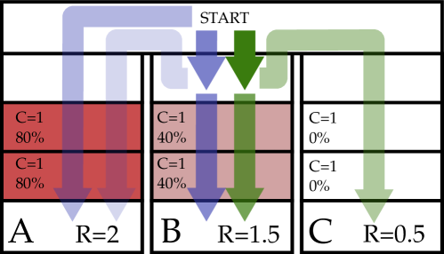
Although the C-POMDP policies generally satisfy the C-POMDP expected cost constraints, the prevalence of high violation rates of C-POMDP policies across the environments strongly suggests that the manifestation of the stochastic self-destruction in C-POMDPs is not an exceptional phenomenon, but intrinsic to the C-POMDP problem formulation. This behavior is illustrated in the Tunnels problem, shown in Figure 2. CGCP (in blue) decides to traverse tunnel of the time even when it observes that is rocky, and traverses tunnel of the time. In contrast, ARCS never traverses tunnel , since such a policy is inadmissible. Instead, it traverses or depending on observation of rocks in tunnel , to maximize rewards while remaining admissible.
Finally, the closed-loop inconsistency of C-POMDP policies is evident when comparing open loop CGCP with closed loop CGCP-CL. In most cases (all except CRS(7,8)), the cumulative reward is decreased when going from CGCP to CGCP-CL, sometimes drastically. The violation rate also decreases, but not to , suggesting that planning with C-POMDPs instead of RC-POMDPs can lead to myopic behavior that cannot be addressed by re-planning. As seen in CE and both CRS, CGCP-CL attains lower reward than ARCS while still having constraint violations. Therefore, even for closed-loop planning, RC-POMDP can be more advantageous than C-POMDP.
Unconstrained POMDP problems
| Env. | Algorithm | Reward | Cost |
|---|---|---|---|
| CE | SARSOP (POMDP) | - | |
| CGCP (C-POMDP) | |||
| Ours (RC-POMDP) | |||
| C-Tiger | SARSOP (POMDP) | - | |
| CGCP (C-POMDP) | 3.2 | ||
| Ours (RC-POMDP) | -1.4 | 3.2 | |
| Tunnels | SARSOP (POMDP) | - | |
| CGCP (C-POMDP) | 1.6 | ||
| Ours (RC-POMDP) | 1.6 | ||
| CRS(4,4) | SARSOP (POMDP) | - | |
| CGCP (C-POMDP) | 2.4 | ||
| Ours (RC-POMDP) | 2.2 | ||
| CRS(5,7) | SARSOP (POMDP) | - | |
| CGCP (C-POMDP) | |||
| Ours (RC-POMDP) | |||
| CRS(5,7) | SARSOP (POMDP) | - | |
| CGCP (C-POMDP) | |||
| Ours (RC-POMDP) |
Next, we evaluate how well the RC-POMDP framework and our proposed algorithm performs for problems that have reduced constraints, so as to trivially become an unconstrained POMDP. We evaluate ARCS (RC-POMDP), CGCP (C-POMDP algorithm) and SARSOP (unconstrained POMDP algorithm) for the same benchmark problems with very high constraint thresholds .
For these problems, all policies are admissible, and ARCS is guaranteed to asymptotically converge to the optimal solution. However, since ARCS needs to keep track of admissible cost values, we utilize a policy tree representation. This representation is less efficient than the -vector policy representation used in SARSOP and CGCP, which allow value improvements at a belief state to directly improve values at other belief states.
Table 2 reports the lower bound reward and upper bound costs computed by each algorithm with a time limit of . As seen in Table 2, our algorithm performs similar to CGCP and the unconstrained POMDP algorithm SARSOP for most smaller problems. The C-Tiger problem benefits greatly from the -vector representation, since the optimal policy repeatedly cycles among a small set of belief states (which our algorithm considers different augmented belief-admissible cost states). For slightly larger problems (CRS(5,7)), the efficient -vector representation and other heuristics of SARSOP (which CGCP takes advantage of, since it repeatedly calls SARSOP) enables much faster convergence than the policy tree-based method of our approach. Nonetheless, as time is increased, our algorithm slowly improves its values.
Overall, ARCS exhibits competitive performance in problems with reduced or no constraints, albeit with less scalability. However, the main advantage of the RC-POMDP formulation is in the careful treatment of constraints to mitigate the pathological behaviors of the C-POMDP formulation, making RC-POMDPs particularly valuable for problems involving nontrivial constraints.
7 Conclusion and Future Work
We introduce and analyze the stochastic self-destruction behavior of C-POMDP policies, and show C-POMDPs may not exhibit optimal substructure. We propose a new formulation, RC-POMDPs, and present an algorithm for RC-POMDPs. Results show that C-POMDP policies exhibit unintuitive behavior not present in RC-POMDP policies, and our algorithm effectively computes policies for RC-POMDPs. We believe RC-POMDPs are an alternate formulation that can be more desirable for some applications.
A future direction is to explore models that exhibit strong cases of stochastic self-destruction, and develop more metrics that signal stochastic self-destruction. Another future direction is to analyze classes (or conditions) of RC-POMDPs that are approximable and to design algorithms that converge for such cases.
Further, our offline policy tree search algorithm can benefit from better policy search heuristics and more efficient policy representations (e.g. finite state controllers). We plan to extend this work by exploring other approaches, such as searching for finite state controllers directly [Wray and Czuprynski, 2022] and online tree search approximations [Lee et al., 2018].
Finally, this work shows that RC-POMDPs can provide more desirable policies than C-POMDPs, but the cost constraints remain on expectation. For some applications, probabilistic or risk measure constraints may be more desirable than expectation constraints. These formulations also benefit from the recursive constraints that we propose for RC-POMDPs.
Acknowledgements.
This work was supported by Strategic University Research Partnership (SURP) grants from the NASA Jet Propulsion Laboratory (JPL) (RSA 1688009 and 1704147). Part of this research was carried out at JPL, California Institute of Technology, under a contract with the National Aeronautics and Space Administration (80NM0018D0004).References
- Chen et al. [2020] Min Chen, Stefanos Nikolaidis, Harold Soh, David Hsu, and Siddhartha Srinivasa. Trust-aware decision making for human-robot collaboration: Model learning and planning. ACM Transactions on Human-Robot Interaction (THRI), 9(2):1–23, 2020.
- Chong et al. [2012] Edwin K.P. Chong, Scott A. Miller, and Jason Adaska. On bellman’s principle with inequality constraints. Operations Research Letters, 40(2):108–113, 2012.
- Cormen et al. [2009] Thomas H. Cormen, Charles E. Leiserson, Ronald L. Rivest, and Clifford Stein. Introduction to Algorithms, 3rd Edition. MIT Press, 2009.
- de Nijs et al. [2021] Frits de Nijs, Erwin Walraven, Mathijs De Weerdt, and Matthijs Spaan. Constrained multiagent markov decision processes: A taxonomy of problems and algorithms. Journal of Artificial Intelligence Research, 70:955–1001, 2021.
- Egorov et al. [2017] Maxim Egorov, Zachary N Sunberg, Edward Balaban, Tim A Wheeler, Jayesh K Gupta, and Mykel J Kochenderfer. Pomdps. jl: A framework for sequential decision making under uncertainty. The Journal of Machine Learning Research, 18(1):831–835, 2017.
- Hauskrecht [1997] Milos Hauskrecht. Planning and control in stochastic domains with imperfect information. PhD thesis, Massachusetts Institute of Technology, 1997.
- Hauskrecht [2000] Milos Hauskrecht. Value-function approximations for partially observable markov decision processes. Journal of artificial intelligence research, 13:33–94, 2000.
- Haviv [1996] Moshe Haviv. On constrained markov decision processes. Operations Research Letters, 19(1):25–28, 1996.
- Isom et al. [2008] Joshua D. Isom, Sean P. Meyn, and Richard D. Braatz. Piecewise linear dynamic programming for constrained POMDPs. In AAAI Conference on Artificial Intelligence, pages 291–296, 2008.
- Jamgochian et al. [2023] Arec Jamgochian, Anthony Corso, and Mykel J. Kochenderfer. Online planning for constrained pomdps with continuous spaces through dual ascent. Proceedings of the International Conference on Automated Planning and Scheduling, 33(1):198–202, Jul. 2023.
- Kaelbling et al. [1998] Leslie Pack Kaelbling, Michael L. Littman, and Anthony R. Cassandra. Planning and acting in partially observable stochastic domains. Artificial Intelligence, 101(1):99–134, 1998.
- Kalagarla et al. [2022] Krishna C. Kalagarla, Kartik Dhruva, Dongming Shen, Rahul Jain, Ashutosh Nayyar, and Pierluigi Nuzzo. Optimal control of partially observable markov decision processes with finite linear temporal logic constraints. In Conference on Uncertainty in Artificial Intelligence, volume 180, pages 949–958. PMLR, 2022.
- Kim et al. [2011] Dongho Kim, Jaesong Lee, Kee-Eung Kim, and Pascal Poupart. Point-based value iteration for constrained POMDPs. In International Joint Conference on Artificial Intelligence, page 1968–1974. AAAI Press, 2011.
- Kurniawati et al. [2008] Hanna Kurniawati, David Hsu, and Wee Sun Lee. SARSOP: Efficient point-based POMDP planning by approximating optimally reachable belief spaces. In Proceedings of Robotics: Science and Systems IV, Zurich, Switzerland, June 2008.
- Lauri et al. [2023] Mikko Lauri, David Hsu, and Joni Pajarinen. Partially observable markov decision processes in robotics: A survey. IEEE Transactions on Robotics, 39(1):21–40, 2023.
- Lee et al. [2018] Jongmin Lee, Geon-hyeong Kim, Pascal Poupart, and Kee-Eung Kim. Monte-carlo tree search for constrained POMDPs. In Advances in Neural Information Processing Systems, page 7934–7943. Curran Associates, Inc., 2018.
- Papakonstantinou and Shinozuka [2014] K.G. Papakonstantinou and M. Shinozuka. Planning structural inspection and maintenance policies via dynamic programming and markov processes. part ii: POMDP implementation. Reliability Engineering & System Safety, 130:214–224, 2014.
- Pendleton et al. [2017] Scott Drew Pendleton, Hans Andersen, Xinxin Du, Xiaotong Shen, Malika Meghjani, You Hong Eng, Daniela Rus, and Marcelo H. Ang. Perception, planning, control, and coordination for autonomous vehicles. Machines, 5(1), 2017.
- Pineau et al. [2006] Joelle Pineau, Geoffrey Gordon, and Sebastian Thrun. Anytime point-based approximations for large POMDPs. Journal of Artificial Intelligence Research, 27:335–380, 2006.
- Piunovskiy and Mao [2000] A.B. Piunovskiy and X. Mao. Constrained markovian decision processes: the dynamic programming approach. Operations Research Letters, 27(3):119–126, 2000.
- Poupart et al. [2015] Pascal Poupart, Aarti Malhotra, Pei Pei, Kee-Eung Kim, Bongseok Goh, and Michael Bowling. Approximate linear programming for constrained partially observable markov decision processes. Proceedings of the AAAI Conference on Artificial Intelligence, 29(1), Mar. 2015.
- Shani et al. [2013] Guy Shani, Joelle Pineau, and Robert Kaplow. A survey of point-based POMDP solvers. Autonomous Agents and Multi-Agent Systems, 27:1–51, 2013.
- Smith and Simmons [2004] Trey Smith and Reid Simmons. Heuristic search value iteration for POMDPs. In Conference on Uncertainty in Artificial Intelligence, page 520–527. AUAI Press, 2004.
- Sondik [1978] Edward J. Sondik. The optimal control of partially observable markov processes over the infinite horizon: Discounted costs. Operations Research, 26(2):282–304, 1978.
- Spaan and Vlassis [2005] Matthijs T. J. Spaan and Nikos Vlassis. Perseus: Randomized point-based value iteration for pomdps. J. Artif. Int. Res., 24(1):195–220, aug 2005.
- Walraven and Spaan [2018] Erwin Walraven and Matthijs T. J. Spaan. Column generation algorithms for constrained pomdps. Journal of Artificial Intelligence Research, 62(1):489–533, 2018.
- Wang et al. [2022] Yizheng Wang, Markus Zechner, John Michael Mern, Mykel J. Kochenderfer, and Jef Karel Caers. A sequential decision-making framework with uncertainty quantification for groundwater management. Advances in Water Resources, 166:104266, 2022.
- Williams [1990] H.P. Williams. Model Building in Mathematical Programming, chapter 3.2.3. Wiley, 5th edition, 1990.
- Wray and Czuprynski [2022] Kyle Hollins Wray and Kenneth Czuprynski. Scalable gradient ascent for controllers in constrained pomdps. In 2022 International Conference on Robotics and Automation (ICRA), pages 9085–9091, 2022.
Appendix A Proofs of Theorem 1
Proof.
Consider an optimal (stochastic) policy . Consider a reachable from by , where has randomization (at least two actions have probabilities in ). Then, can be equivalently represented as a mixture over policies that deterministically selects a unique action at but is the same (stochastic) policy as everywhere else. That is, is a mixed policy over the set of policies that have a deterministic action at and at every other history. Let represent the non-zero probability of choosing at . Then, and .
We show that all the policies must be admissible in order for to be admissible. Suppose there exists an inadmissible policy . That is, there exists a history s.t. Eq. (11) or (14) is violated by .
For , is only reachable by taking action at , since each policy in takes a different action at , and so their reachable history spaces are different. Only the inadmissible is executed from when it is reached probablistically, and . This means that Eq.(11) is violated at depth , so is inadmissible, which is a contradiction.
Similarly, for , if (Eq. (14) are violated),
since
This can be seen by rearranging Eq. (13) and
. That is, Eq. (14) is violated at time step , so is inadmissible, which is again a contradiction. Hence, each is admissible.
Since , determinism at is sufficient, i.e., obtain a new with one less randomization. Repeating the same process for all histories reachable from by with randomization obtains a deterministic optimal policy. ∎
Appendix B Proof of Theorem 2
Proof.
Let denote the action set computed during the Bellman backup operation on to obtain .
We first show that , i.e., the optimality after a Bellman backup operation is preserved.
Consider any . By optimality of , Suppose ,
which is a contradiction, so . However, we have that
Now, we show that , i.e., the admissibility of the optimal policy after a Bellman backup operation is preserved.
Let be the first augmented belief state from in a belief trajectory such that does not satisfy Eq. 14, i.e., satisfies Eq. 14 , and .
Therefore,
Consider the augmented belief state that transitions to under some action and observation .
Note that is finite for finite . So and therefore cannot be reachable under . By induction, we have that ,
∎
B.1 Proof of Theorem 3
Proof.
Suppose that is well behaved.
Denote . Then, for all , . A lack of admissible policy implies that there are no actions from that leads to admissibility. This implies that , there exists at least successor augmented belief state , such that . Therefore,
Therefore, we have that for all ,
Next, denote . Consider any , and . There must exist at least action that is part of an admissible policy, i.e., . Therefore, at
Since any are inadmissible and will not be selected during the Bellman backup operation, we can exclude them from the set of actions without loss of generality. Denote as the set of actions that may be selected at . Then, for all ,
Consider . We have that
By induction, , so the policy remains admissible after applying . Therefore, we can write
Note that this is the standard Bellman operator for an unconstrained discounted-sum POMDP over the set of admissible augmented belief states. From the results of the Bellman operator for a POMDP [Hauskrecht, 1997], is a contraction mapping and has a single, unique fixed point, i.e., for an optimal , . Since , we have that
∎
Appendix C ARCS Pseudocode
Global variables:
Let
SAMPLE()
SampleHeu().
SampleRandom()
Global variables:
Let
BACKUP()
Global variables:
PRUNE()
Appendix D Proof of Lemma 1
Proof.
Given a maximum one-step cost for and a non-negative admissible cost , a lower bound on the admissible horizon can be obtained as follows. The -step admissible horizon from each leaf node is the largest such that
The LHS is a finite geometric series:
| (23) |
Hence, the largest integer that satisfies Eq. (23) is
Also, we obtain the -admissibility condition on by setting in Eq. (23):
Next, when , since costs are non-negative, the minimum cost policy obtains cost at every future belief, and hence .
Finally, when admissible cost is negative, the constraints are trivially violated, and hence . ∎
Appendix E Proof of Proposition 3
Proof.
During search, the pruning criteria prunes policies according to four cases. We show that these four cases only prunes sub-optimal policies and inadmissible policies.
-
1.
.
It is easy to see that if , it is guaranteed that no admissible policies exist from , so we can prune and its subtree. -
2.
At node , actions and are compared. Specifically, is compared with , if (the policy from taking is admissible). The node-action is pruned if .
There are two cases to consider: (i) and (ii) . In case (i), . is a valid upper bound of the Q reward-value of taking action as a consequence of Lemma 2. In case (ii), , is also a valid upper bound of the Q reward-value of taking action . For a node with , We show that is an upper bound on . That is, if , we have that for an optimal policy starting from with optimal reward-value and cost-value ,(24) This can be seen by noting that the BACKUP step performs an RC-POMDP Bellman backup. If the policy is in fact admissible (since is an underestimate), then the results from Lemma 2 hold. If the policy is not admissible, the optimal reward-value of an admissible policy from that node cannot be higher than (and the optimal cost-value cannot be higher than ), since an admissible policy satisfies more constraints than a finite -admissible one. In both cases, is strictly a better action than , so taking action at node cannot be part of an optimal policy.
-
3.
If all node-actions are pruned, is also pruned.
No actions are admissible from so it is inadmissible. -
4.
is pruned if any successor node from taking action is pruned.
A successor node is pruned (case 1 or 3), so this policy is not admissible.
∎
Appendix F Proof of Lemma 2
Proof.
The proof relies on the result of Theorem 1. that for admissibility constraint , deterministic policies are sufficient for optimality. That is, it is sufficient to provide upper and lower bounds over deterministic policies.
We first show that the initial bounds for a new (leaf) node (Algorithm 3) are true bounds on the optimal policy.
and are initialized with the Fast Informed Bound with the unconstrained POMDP problem, separately for reward maximization and cost minimization. The Fast Informed Bound provides valid upper bounds on reward-value (and lower bounds on cost-value of a cost-minimization policy, which in turn is a lower bound on cost-value for an optimal RC-POMDP policy) Hauskrecht [2000]. The upper bound on the optimal reward-value for the reward-maximization unconstrained POMDP problem is also an upper bound on the optimal reward-value for an RC-POMDP which has additional constraints. Similarly, the lower bound on the optimal cost-value for the cost-minimization unconstrained POMDP problem is also a lower bound on the cost-value of an optimal RC-POMDP policy which has additional constraints.
and are computed using the minimum cost policy . This minimum cost policy is an alpha-vector policy, which is an upper bound on the cost-value function Hauskrecht [2000], so is an upper bound on the cost-value when following the minimum cost policy. It can also be seen that the value from following the same policy is a valid bound on the optimal reward-value function from that node. Finally, the admissible horizon guarantee is initialized using the results from Lemma 1, which is shown to be a lower bound on the true admissible horizon following the minimum cost policy.
Next, we show that performing the BACKUP step (Algorithm 4 maintains the validity of the bounds. Recall the condition of this lemma that admissible horizon guarantee for the node . Thus, after the backup step, the admissible horizon guarantee remains at . From the proof of Theorem 2, the RC-POMDP Bellman backup satisfies Bellman’s Principle of Optimality and is a contraction mapping within the space of admissible value functions (and hence policies).
Let be the value after the BACKUP step, which performs a Bellman backup on :
Since is a contraction mapping within the space of admissible policies, we see that:
Therefore, for , we have that for an optimal policy starting from with optimal reward-value and cost-value ,
∎
Appendix G Proof of Theorem 4
Proof.
There are two termination criteria for ARCS, of which both must be true before termination. ARCS terminates when (1) it finds an admissible policy, and (2) the policy is -optimal, that is when . We first discuss admissibility, then -optimality.
(1) ARCS can terminate when it finds an admissible policy, i.e., . ARCS finds an admissible policy when every leaf node under the policy satisfies (i) Eq. (20), or (ii) .
We prove that this is a sound condition, i.e., if the (i) and (ii) hold for every leaf node , the computed policy is indeed admissible. As proven in Lemma 1, the admissible horizon guarantee for a leaf node is a conservative under-approximation. Therefore, a leaf node with indeed means that we have found an admissible policy from (with ). Suppose all leaf nodes have . The worst-case back-propagation of admissible horizon guarantee up the tree is sound, since a non-leaf node only has if all its leaf nodes have and Eq. (9) is satisfied at that node (Lines 9-18 in Algorithm 4). Therefore, if , the policy is admissible, and ARCS can terminate if .
(2) ARCS can terminate when the gap criterion at the root is satisfied, that is when .
If , the policy at is admissible, which implies every history-belief reachable under the policy tree is admissible. From Lemma 2, this implies that for all nodes, are valid bounds on the optimal value function. Thus, and are valid bounds on the optimal value function from , and so, an -optimal policy is indeed found.
Therefore, if ARCS terminates, the computed solution is an admissible -optimal policy. ∎
Appendix H Experimental Evaluation
H.1 Implementation details
The code for each algorithm implementation can be found in the attached supplementary material. Here, we detail parameters and implementation of the algorithms. For hyper-parameter tuning, we used the default parameters for ARCS. For the rest of the algorithms, the values of the hyper-parameters were chosen based empirical evaluations, and fixed for the experiments. For each environment, we used a maximum time step of during evaluation. Except for the Tiger problem, all algorithms reached terminal states before time steps in these problems or produced a policy which stayed still at time steps.
H.1.1 ARCS
We implemented ARCS as described. We used the Fast Informed Bound for the initialization of upper bound on reward value and lower bound on cost value. We used SARSOP for the computation of the minimum cost policy. We set the SARSOP hyperparameter for our experiments, the same value as Kurniawati et al. [2008]. We used a uniform randomization ( probability) between heuristic sampling and random sampling during planning, and we leave an analysis on how the randomization weight may affect planning efficiency to future work.
H.1.2 CGCP
We implemented CGCP and adapted it for discounted infinite horizon problems, using Alg. 5 in Walraven and Spaan [2018] as a basis. However, we use the discounted infinite horizon POMDP solver SARSOP Kurniawati et al. [2008] in place of a finite horizon PBVI. Our method of constructing policy graphs also differs, as the approach described is for finite horizon problems. We check for a return to beliefs previously visited under the policy in order to reduce the size of the graph. A maximum time of seconds was used for CGCP. For each SARSOP iteration within CGCP, seconds was given initially, while the solve time was incremented by seconds every time that the dual price remained the same. Additionally, CGCP was limited to iterations. In an effort to reduce computation time, policy graph evaluation and SARSOP search was limited to depth (the same as the monte carlo evaluation depth) in all domains except the RockSample domains, which were allowed unlimited depth.
For the Tunnels benchmark, monte carlo simulations to depth were used in place of a policy graph to estimate the value of policies. This was due to the inability of the policy graphs to estimate the value of some infinite horizon POMDP solutions which do not lead to terminal states or beliefs which have already appeared in the tree.
H.1.3 CGCP-CL
CGCP-CL uses the same parameters as CGCP, but re-plans at every time step.
H.1.4 No-regret Learning Algorithm
We implemented the no-regret learning algorithm from [Kalagarla et al., 2022]. We used SARSOP as the unconstrained POMDP solver, and monte carlo simulations to estimate the value of policies.
H.1.5 CPBVI
We implemented CPBVI based on Kim et al. [2011]. The algorithm generates a set of reachable beliefs before performing iterations of approximate dynamic programming on the belief set. However, the paper did not include full details on belief set generation and alpha-vector set initialization.
The paper cited Pineau et al. [2006] for their belief set description, and so we followed Pineau et al. [2006] by expanding greedily towards achieving uniform density in the set of reachable beliefs. This is done by randomly simulating a step forward from a node in the tree, thereby generating candidate beliefs, and keeping the belief that is farthest from any belief already in the tree. We repeat this expansion until the desired number of beliefs have been added to the tree.
To address initialization, we adopted the blind lower bound approach. This approach represents the lower bound with a set of alpha-vectors corresponding to each action in . Each alpha-vector is generated under the assumption that the same action is taken forever. To compute an alpha-vector corresponding to a given action, we first compute the best-action worst-state (BAWS) lower bound. This is done by evaluating the discounted reward obtained by taking the best action in the worst state forever. We can then update the BAWS alpha-vectors by performing value backups until convergence.
The CPBVI algorithm involves the computation of a linear program (LP) to obtain the best action at a given belief. One of the constraints asserts that the convex combination of cost alpha-vectors evaluated at a given belief must be equal to or less than the admissible cost associated with , which is used in CPBVI’s heuristic approach. However, if , the LP becomes infeasible. The case of is possible since no pruning of beliefs is conducted. The paper did not provide details to account for this situation. To address this, if the LP is infeasible, we output the action with the lowest cost, akin to ARCS’ minimum cost policy method when no policy is admissible.
H.1.6 CPBVI-D
CPBVI computes stochastic policies. We modify CPBVI to only compute deterministic policies with the following details. Instead of solving the LP to generate a stochastic action, we solve the for the single highest value action subject to the cost-value constraint.
Although both CPBVI and CPBVI-D theoretically have performance insensitive to random seed initialization, both algorithms are sensitive to the number of belief parameter during planning. With too few beliefs selected for a problem, both algorithms cannot search the problem space sufficiently. With too many beliefs selected, the time taken for belief selection is too high for the moderately sized problems of CRS and Tunnels. Therefore, we tuned and chose a belief parameter of that allows finding solutions in the planning time of . Note that even with a small number of beliefs of , CPBVI routinely overruns the planning time limit during its update step.
H.2 Environment details
Except for the RockSample environment, our environments do not depend on randomness. For each RockSample environment of which rock location depends on randomness, we used the rng algorithm MersenneTwister with a fixed seed to generate the RockSample environments.
H.2.1 Counterexample Problem
The counterexample POMDP in Figure 1 uses a discount of . In the experiments, we used a discount factor of to approximate a discount of . It is modeled as an RC-POMDP as follows.
States are enumerated as with actions following as and observations being noisy indicators for whether or not a state is rocky.
States and indicate whether cave 1 or cave 2 contains rocky terrain, respectively. Taking action circumvents the caves unilaterally incurring a cost of and transitioning to terminal state . Taking action moves closer to the caves where deterministically transitions to . In this transition, the agent is given an 85% accurate observation of the true state.
At this new observation position, the agent is given a choice to commit to one of two caves where indicates that cave 1 contains rocks and indicates that cave 2 contains rocks. Action moves through cave 1 and moves through cave 2. Moving through rocks incurs a cost of while avoiding them incurs no cost. Taking action at this point, regardless of true state, gives a reward of . States and unilaterally transition to terminal state .
H.2.2 Tunnels Problem
The tunnels problem is modeled as an RC-POMDP as follows. As depicted in figure 2, the tunnels problem consists of a centralized starting hall that funnels into 3 separate tunnels. At the end of tunnels 1,2,and 3 lie rewards 2.0, 1.5 and 0.5 respectively. However, with high reward also comes high cost as tunnel 1 has a 80% probability of containing rocks and tunnel 2 has a 40% probability of containing rocks while tunnel 3 is always free of rocks. If present, the rocks fill 2 steps before the reward location at the end of a tunnel and a cost of 1 is incurred if the agent traverses over these rocks. Furthermore, a cost of 1 is incurred if the agent chooses to move backwards.
The only partial observability in the state is over whether or not rocks are present in tunnels 1 or 2. As the agent gets closer to the rocks, accuracy of observations indicating the presence of rocks increases.
H.3 Experiment Evaluation Setup
We implemented each algorithm in Julia using tools from the POMDPs.jl framework Egorov et al. [2017], and all experiments were conducted single-threaded on a computer with two nominally 2.2 GHz Intel Xeon CPUs with 48 cores and 128 GB RAM. All experiments were conducted in Ubuntu 18.04.6 LTS. For all algorithms except CGCP-CL, solve time is limited to seconds and online action selection to seconds. For CGCP-CL, seconds was given for each action (recomputed from scratch). We simulate each policy times, except for CGCP-CL, which is simulated times due to the time taken for re-computation of the policy at each time step. The full results with the mean and standard error of the mean for each metric are shown in Table. 3.
| Environment | State/Action/Obs | Algorithm | Violation Rate | Cumulative Reward | Cumulative Cost |
|---|---|---|---|---|---|
| CE | CGCP | ||||
| CGCP-CL | |||||
| () | CPBVI | ||||
| CPBVI-D | |||||
| EXP-Gradient | |||||
| Ours | |||||
| C-Tiger | CGCP | ||||
| CGCP-CL | |||||
| () | 2 / 3 / 2 | CPBVI | |||
| CPBVI-D | |||||
| EXP-Gradient | |||||
| Ours | |||||
| C-Tiger | CGCP | ||||
| CGCP-CL | |||||
| () | 2 / 3 / 2 | CPBVI | |||
| CPBVI-D | |||||
| EXP-Gradient | |||||
| Ours | |||||
| CRS(4,4) | CGCP | ||||
| CGCP-CL | |||||
| () | 201 / 8 / 3 | CPBVI | |||
| CPBVI-D | |||||
| EXP-Gradient | |||||
| Ours | |||||
| CRS(5,7) | CGCP | ||||
| CL-CGCP | |||||
| () | 3201 / 12 / 3 | CPBVI | |||
| CPBVI-D | |||||
| EXP-Gradient | |||||
| Ours | |||||
| CRS(7,8) | CGCP | ||||
| CL-CGCP | |||||
| () | 12545 / 13 / 3 | CPBVI | |||
| CPBVI-D | |||||
| EXP-Gradient | |||||
| Ours | |||||
| CRS(11,11) | CGCP | ||||
| CL-CGCP | - | - | - | ||
| () | 247809 / 16 / 3 | CPBVI | |||
| CPBVI-D | |||||
| EXP-Gradient | |||||
| Ours | |||||
| Tunnels | CGCP | ||||
| CL-CGCP | |||||
| () | 53 / 3 / 5 | CPBVI | |||
| P(correct obs) = | CPBVI-D | ||||
| EXP-Gradient | |||||
| Ours | |||||
| Tunnels | CGCP | ||||
| CL-CGCP | |||||
| () | 53 / 3 / 5 | C-PBVI | |||
| EXP-Gradient | |||||
| P(correct obs) = | CPBVI-D | ||||
| Ours |