Reduction principle for functionals of strong-weak dependent vector random fields
Abstract
We prove the reduction principle for asymptotics of functionals of vector random fields with weakly and strongly dependent components. These functionals can be used to construct new classes of random fields with skewed and heavy-tailed distributions. Contrary to the case of scalar long-range dependent random fields, it is shown that the asymptotic behaviour of such functionals is not necessarily determined by the terms at their Hermite rank. The results are illustrated by an application to the first Minkowski functional of the Student random fields. Some simulation studies based on the theoretical findings are also presented.
keywords:
[class=MSC]keywords:
arXiv:1803.11271 \startlocaldefs \endlocaldefs
t1Supplementary Materials R code used for simulations in this article is available in the folder “Research materials” from \hrefhttps://sites.google.com/site/olenkoandriy/.
and
a]La Trobe University
1 Introduction
In various applications researchers often encounter cases involving dependent observations over time or space. Dependence properties of a random process are usually characterized by the asymptotic behaviour of its covariance function. In particular, a stationary random process , is called weakly (short-range) dependent if its covariance function is integrable, i.e. . On the other hand, possesses strong (long-range) dependence if its covariance function decays slowly and is non-integrable. An alternative definition of long-range dependence is based on singular properties of the spectral density of a random process, such as unboundedness at zero (see Doukhan et al. (2002); Souza (2008); Leonenko and Olenko (2013)).
Long-range dependent processes play a significant role in a wide range of areas, including finance, geophysics, astronomy, hydrology, climate and engineering (see Leonenko (1999); Ivanov and Leonenko (1989); Doukhan et al. (2002)). In statistical applications, long-range dependent models require developing new statistical methodologies, limit theorems and parameter estimates compared to the weakly dependent case (see Ivanov and Leonenko (1989); Worsley (1994); Leonenko and Olenko (2013); Beran et al. (2013)).
In statistical inference of random fields, limit theorems are the central topic. These theorems play a crucial role in developing asymptotic tests in the large sample theory. The central limit theorem (CLT) holds under the classical normalisation when the summands or integrands are weakly dependent random processes or fields. This result was proved by Breuer and Major (1983) for nonlinear functionals of Gaussian random fields. A generalisation for stationary Gaussian vector processes was obtained in de Naranjo (1995), for integral functionals of Gaussian processes or fields in Chambers and Slud (1989), Hariz (2002), Leonenko and Olenko (2014), for quasi-associated random fields under various conditions in Bulinski et al. (2012) and Demichev (2015). Some other CLTs for functionals of Gaussian processes or fields can be found in Doukhan and Louhichi (1999); Coulon-Prieur and Doukhan (2000) and Kratz and Vadlamani (2018).
The non-central limit theorems arise in the presence of long-range dependence. They use normalising coefficients different than in the CLT and have non-Gaussian limits. These limits are known as Hermite type distributions. A non-Gaussian asymptotic was first obtained in Rosenblatt (1961) as a limit for quadratic functionals of stationary Gaussian sequences. The article Taqqu (1975) continued this research and investigated weak limits of partial sums of Gaussian processes using characteristic functions. The Hermite processes of the first two orders were used. Later on, Dobrushin and Major (1979) and Taqqu (1979) established pioneering results in which asymptotics were presented in terms of multiple Wiener-Itô stochastic integrals. A generalisation for stationary Gaussian sequences of vectors was obtained in Arcones (1994) and Major (2019). Multivariate limit theorems for functionals of stationary Gaussian series were addressed under long-range dependence, short-range dependence and a mixture of both in Bai and Taqqu (2013). The asymtotices for Minkowski functionals of stationary and isotropic Gaussian random fields with dependent structures were studied in Ivanov and Leonenko (1989). Leonenko and Olenko (2014) obtained the limit theorems for sojourn measures of heavy-tailed random fields (Student and Fisher-Snedecor) under short or long-range dependence assumptions. Excellent surveys of limit theorems for shortly and strongly dependent random fields can be found in Anh et al. (2015); Doukhan et al. (2002); Ivanov and Leonenko (1989); Leonenko (1999); Spodarev (2014).
The reduction theorems play an important role in studying the asymptotics for random processes and fields. These theorems show that the asymptotic distributions for functionals of random processes or fields coincide with distributions of other functionals that are much simpler and easier to analyse. The CLT can be considered as the “extreme” reduction case, when, due to weak dependence and despite the type of functionals and components distributions, asymptotics are reduced to the Gaussian behaviour. The classical non-central limit theorems are based on another “proper” reduction principle, when the asymptotic behaviour is reduced only to the leading Hermite term of nonlinear functionals. Recently, Olenko and Omari (2019) proved the reduction principle for functionals of strongly dependent vector random fields. Components of such vector fields can possess different long-range dependences. It was shown that, in contrast to the scalar cases, the limits can be degenerated or can include not all leading Hermite terms.
The available literature, except a few publications, addresses limit theorems and reduction principles for functionals of weakly or strongly dependent random fields separately. For scalar-valued random fields it is sufficient as such fields can exhibit only one type of dependence. However, for vector random fields there are various cases with different dependence structures of components. Such scenarios are important when one aggregates spatial data with different properties. For example, brain images of different patients or GIS data from different regions. Another reason for studying such models is constructing scalar random fields by a nonlinear transformation of a vector field. This approach was used to obtain non-Gaussian fields with some desirable properties, for example, skewed or heavy tailed marginal distributions, see Example 1, Theorem 5 and Leonenko and Olenko (2014).
This paper considers functionals of vector random fields which have both strongly and weakly dependent components. The results in the literature dealt with cases where the interplay between terms at the Hermite rank level and the memory parameter (covariance decay rate) of a Gaussian field completely determines the asymptotic behavior. This paper shows that in more general settings terms at non-Hermite rank levels can interplay with the memory parameter to determine the limit. As an application of the new reduction principle we provide some limit theorems for vector random fields. In particular, we show that it is possible to obtain non-Gaussian behaviour for the first Minkowski functional of the Student random field built on different memory type components. It contrasts to the known results about the cases of same type memory components in Leonenko and Olenko (2014) where, despite short or long range dependence, only the Gaussian limit is possible.
The remainder of the paper is organised as follows. In Section 2 we outline basic notations and definitions that are required in the subsequent sections. Section 3 presents assumptions and main results for functionals of vector random fields with strongly and weakly dependent components. Sections 4 gives the proofs. Section 5 demonstrates some numerical studies. Short conclusions and some new problems are presented in Section 6.
2 Notations
This section presents basic notations and definitions of the random field theory and multidimensional Hermite expansions. Also, we introduce the definition and basic properties of the first Minkowski functional (see Adler and Taylor (2009)). Denote by and the Lebesgue measure and the Euclidean distance in , respectively. The symbol denotes constants that are not important for our exposition. Moreover, the same symbol may be used for different constants appearing in the same proof. We assume that all random fields are defined on the same probability space .
Definition 1.
Bingham et al. (1989) A measurable function is slowly varying at infinity if for all ,
A real-valued random field , satisfying is said to be homogeneous and isotropic if its mean function is a constant and the covariance function depends only on the Euclidean distance between and .
Let , , be a measurable mean square continuous zero-mean homogeneous isotropic real-valued random field (see Ivanov and Leonenko (1989); Leonenko (1999)) with the covariance function
where and is the Bessel function of the first kind of order . The finite measure is called the isotropic spectral measure of the random field , .
The spectrum of the random field is absolutely continuous if there exists a function , , such that
The function is called the isotropic spectral density of the random field .
A random field with an absolutely continuous spectrum has the following isonormal spectral representation
where is the complex Gaussian white noise random measure on .
Let be a Jordan-measurable compact connected set with , and contains the origin in its interior. Also, assume that , , is the homothetic image of the set , with the centre of homothety in the origin and the coefficient , that is, .
Definition 2.
The first Minkowski functional is defined as
where is the indicator function and is a constant.
The functional has a geometrical meaning, namely, the sojourn measure of the random field .
In the following we will use integrals of the form with various integrable Borel functions . Let two independent random vectors and in be uniformly distributed inside the set . Consider a function . Then, we have the following representation
| (2.1) |
where , , denotes the density function of the distance between and .
Using (2) for and one obtains for
| (2.2) |
Let be a -dimensional zero-mean Gaussian vector and , , , be the Hermite polynomials, see Taqqu (1977).
Consider
where , and all for
The polynomials form a complete orthogonal system in the Hilbert space
where
An arbitrary function admits an expansion with Hermite coefficients , given as the following:
where and
Definition 3.
The smallest integer such that for all , , but for some is called the Hermite rank of and is denoted by .
In this paper, we consider Student random fields which are an example of heavy-tailed random fields. To define such fields, we use a vector random field , , with where , , are independent homogeneous isotropic unit variance Gaussian random fields.
Definition 4.
The Student random field (t-random field) , is defined by
3 Reduction principles and limit theorems
In this section we present some assumptions and the main results. We prove a version of the reduction principle for vector random fields with weakly and strongly dependent components.
In the following we will use the notation
for a vector random field with components.
Assumption 1.
Let be a vector homogeneous isotropic Gaussian random field with independent components, and a covariance matrix such that and
where , and are unit matrices of size , and , respectively, , , are slowly varying functions at infinity.
Remark 1.
If Assumption 1 holds true the diagonal elements of the covariance matrix are integrable for the first elements of , which corresponds to the case of short-range dependence, and non-integrable for the other elements, which corresponds to the case of long-range dependence. For simplicity, this paper investigates only the case of uncorrelated components.
Remark 2.
Consider the following random variables:
and
where are the Hermite coefficients and is the Hermite rank of the function . Then
Remark 3.
The random variable is correctly defined, finite with probability 1 and in the mean square sense, see §3, Chapter IV in Gihman and Skorokhod (2004).
We will use the following notations. Consider the set
Let
Note that and there are cases when can be reached at multiple . Therefore, we define the sets
and
Also, we define the random variable
The random variable if and only if .
Theorem 1 in Olenko and Omari (2019) gives a reduction principle for vector random fields with strongly dependent components. The following result complements it for the case of random fields with strongly and weakly dependent components.
Theorem 1.
Suppose that a the vector random field , , satisfies Assumption 1, and there is at least one such that . If for a limit distribution exists for at least one of the random variables
then the limit distribution of the other random variable exists as well, and the limit distributions coincide. Moreover, the limit distributions of
are the same.
Remark 4.
It will be shown in the proof that the assumptions of Theorem 1 guarantee that .
Remark 5.
It follows from the asymptotic analysis of the variances in Theorem 1 that
Assumption 2.
Components , , of have the spectral density , , such that
where
Denote the Fourier transform of the indicator function of the set by
Let us define the following random variable
| (3.2) |
where is the Wiener measure on and denotes the multiple Wiener-Itô integral.
Theorem 2.
A popular recent approach to model skew distributed random variables is a convolution , where is Gaussian and is continuous positive-valued independent random variables. In this case the probability density of has the form , where is the pdf of and is the cdf of , which controls the skewness, see Arellano-Valle and Genton (2005); Azzalini and Capitanio (2014) and Amiri et al. (2019). This approach can be extended to the case of random fields as , , resulting in with skewed marginal distributions. In the example below we use and show that contrary to the reduction principle for strongly dependent vector random fields in Olenko and Omari (2019) it is not enough to request . The assumption of the existence of satisfying in Theorem 1 is essential.
Example 1.
Let , and . In this case and , but . So, the assumption of Theorem 1 does not hold and
which is indeed different from the Gaussian limit that is expected for the case .
To address situations similar to Example 1 and investigate wider classes of vector field we introduce the following modification of Assumption 1.
Assumption 1′.
Let , , be a vector homogeneous isotropic Gaussian random field with independent components, and a covariance matrix such that and
where , and , .
Remark 6.
Under Assumption 1′ the components are still strongly dependent, but , , do not necessarily preserve strong dependence. If the Hermite polynomials of become weakly dependent.
The following modifications of , , and will be used to match Assumption 1′:
and
In the following we consider only the cases The case when the sum equals requires additional assumptions, see Section 6, and will be covered in other publications.
Now, we are ready to formulate a generalization of Theorem 1.
Theorem 3.
Suppose that a vector random field , , satisfies Assumption 1′ and . If a limit distribution exists for at least one of the random variables
then the limit distribution of the other random variable exists as well, and the limit distributions coincide when .
Assumption 2′.
Components , , of have spectral densities , , such that
Theorem 4.
Corollary 1.
Remark 7.
It is possible to obtain general versions of Theorems 2 and 4 by removing the assumptions about and and requesting only or respectively. However, it requires an extension of the known non-central limit theorems for vector fields from the discrete to continuous settings, see Section 6. Also, in such general cases the summands in the limit random variables analogous to (3.3) would be dependent.
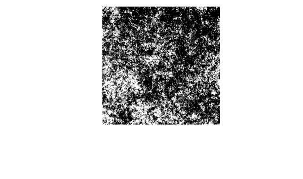
As an example we consider the first Minkowski functional of Student random fields. The special cases of only weakly or strongly dependent components were studied in Leonenko and Olenko (2014). It was shown that in the both cases the asymptotic distribution is , but with different normalisations, see Theorems 3 and 6 in Leonenko and Olenko (2014). Figure 1 gives a two-dimensional excursion set above the level for a realisation of a long-range dependent Cauchy model. The excursion set is shown in black colour. More details are provided in Section 5.
The next result shows that for the first Minkowski functional of t-fields obtained from vector random fields with both weakly and strongly dependent components the limit distributions can be non-Gaussian.
Theorem 5.
Let Assumption 2′ hold true, , , . Then the random variable
converges in distribution to the random variable
where are independent copies of the random variable
and is the signum function.
Remark 8.
Random variables have the Rosenblatt-type distribution, see Anh et al. (2015).
Remark 9.
As , the first component is weakly dependent and the remaining components , , are strongly dependent.
4 Proofs of the results from Section 3
Proof of Theorem 1.
First we study the behaviour of . Note, that
Let us denote the sets as follows
and
Then and can be written as
Note, that all components , , in the first term are weakly dependent and the variance is equal
Let and . The Jacobian of this transformation is . By denoting , , then can be rewritten as
It follows from and by Remark 5 that for weakly dependent components we get
Noting that
one obtains the following asymptotic behaviour of
| (4.1) |
In contrast, the components , , in the second term are strongly dependent and can be obtained as follows
By (2) we get
Noting that by Theorem 2.7 in Seneta (1976) we obtain
| (4.2) |
where . By (2) and the condition the coefficient is finite as
There are strongly and weakly dependent components in the term and its variance can be rewritten as follows
| Var | ||||
| (4.3) |
where
| (4.4) |
and
Note, that by properties of slowly varying functions is also a slowly varying function.
If in (4) the power is greater than then this case is analogous to the case of with short-range dependence and similar to (4.1) one obtains
| (4.5) |
This is indeed the case for as and .
Note, that by the conditions of the theorem . Now, by properties of slowly varying functions (see Preposition 1.3.6 in Bingham et al. (1989)), we get
| (4.6) |
By (4.2) and (4.5) we also obtain
| (4.7) |
Note, that
Using the Cauchy–Schwarz inequality by (4.6) and (4.7) we get for that
| (4.8) |
Therefore, combining the above results we obtain
| (4.9) |
Now, we study the behaviour of . Similarly to , to investigate we define the following sets
and
Then can be written as
Hence,
The components , , in are weakly dependent and is given by
| (4.10) |
As and we can estimate the expression in (4.10) by
It follows from this estimates and the asymptotic (4.1) for that
| (4.11) |
In the term the components are strongly and weakly dependent random fields. Similarly to the case of we obtain that is equal
where
and
is a slowly varying function.
Now, as then and similar to (4.1) the variance has the asymptotic behaviour
| (4.12) |
Note, that all assumptions of Theorem 1 in Olenko and Omari (2019) are satisfied in our case as , , and then
Therefore, by Theorem 1 in Olenko and Omari (2019) we get
| (4.13) |
Finally, combining (4.11), (4.13) (4.12) and applying the Cauchy–Schwarz inequality analogously to one obtains that , which proves the asymptotic equivalence of and
Proof of Theorem 2.
By Remark 5, , , and hence and have the same limit distribution.
is a sum of independent terms of the form
It follows from Theorem 5 in Leonenko and Olenko (2014) that for the independent components and for each
which completes the proof. ∎
Proof of Example 1.
Proof of Theorem 3.
It follows from that there is at least one such that . Moreover, as can be obtained only for with and then is a finite set. Hence, it holds , where
and
are disjoint sets.
Using the Hermite expantion of we obtain
Analogously to (4) and (4) the variance of each summand in has the form
Then, similarly to (4.1) and (4.2) we obtain that and , , and each term in has the variance that is asymptotically equivalent to
By the definition of , , we get
Using the Cauchy-Schwarz inequality analogously to (4.8) one obtains
Finally, noting that completes the proof. ∎
Proof of Theorem 4.
By Theorem 3
have the same limit distribution if it exists. It follows from the structure of that is a sum of terms
By Theorem 5 in Leonenko and Olenko (2014) for
| (4.15) |
Note, that from , if , follows that , if . Therefore, the term in (4.15) are independent for different .
From the existence of it follows that
| (4.16) |
for and .
As then and all coefficients are finite.
Proof of Theorem 5.
As is an even function of , , then for all such that for some . For such that for some , we obtain
Now we investigate as a function of :
where .
Using the formula for the central absolute moments we obtain
Thus, is a strictly increasing function on and it decreases on . Note, that and by the formula for the central absolute moments
Therefore, for and such that for some . Hence, we obtain that , and . The application of Theorem 4 completes the proof. ∎
5 Simulation studies
In the following numerical examples we use the generalised Cauchy family covariance, see Gneiting and Schlather (2004) and Schlather et al. (2019), to model components of , .
The Cauchy covariance function is
To simulate long-range dependent components we consider . In this range of the covariance function is non-integrable. For the case of weakly dependent components we use which gives integrable covariance functions.
Limit distributions were investigated using the following procedure. Random fields were simulated on the plane i.e. using the square observation window The R software package RandomFields (see Schlather et al. (2019)) was used to simulate , , from Cauchy models.
Example 1′.
Here we illustrate the results in Example 1. The Cauchy model was used to simulate , , , satisfying Assumption 1′ with and respectively. realisations of , and were generated for the large value to compute distributions of , and respectively.
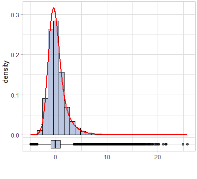
Notice that the random field has skewed marginal distributions, see Figure 2. The coefficient of the skewness equals , i.e. the marginal distribution of has a heavy right-hand tail.
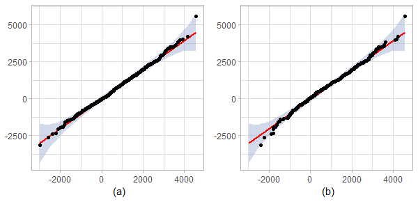
To compare empirical distributions, Q-Q plots of realisations of versus realisations of and are produced in Figure 3. As large and the number of realisations were selected for simulations these empirical distributions are close to the corresponding asymptotic distributions.
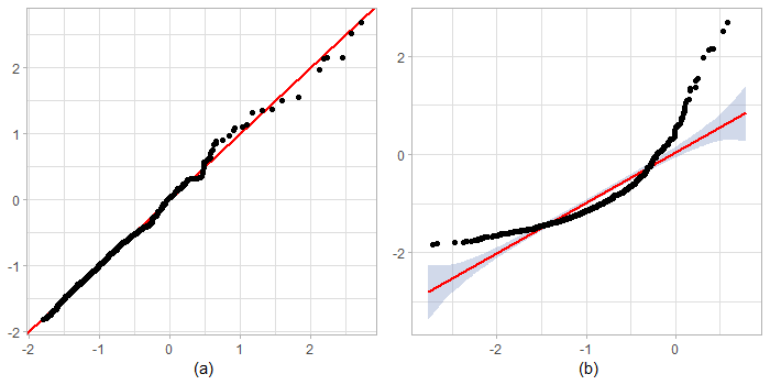
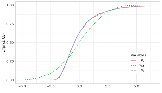
It is clear from Figure 3(a) that asymptotic distributions of and are close and the reduction principle works. The Kolmogorov-Smirnov test confirms this result with -value , see also Figure 4 where the plots of empirical cdfs of and are almost identical. However, Figure 3(b) shows that the distributions of and are different, i.e. asymptotic behaviour of functionals of vector random fields with weak-strong dependent components is not necessarily determined by their Hermite ranks. This result is also confirmed by the Kolmogorov-Smirnov -value and Figure 4.
Example 2.
This example illustrates Theorem 5. For , and we simulated realisations of the field , For each realisation the area of the excursion set above the level was computed. Figure 5 presents the Q-Q plots with pointwise normal confidence bands for empirical distributions of excursion areas.
The short-range dependent Cauchy model was used to generate realisations of with for all , . Figure 5(a) shows that all the quantiles lie within the confidence bands which confirms that the first Minkowski functional is Gaussian.
Another set of realisations of was generated using the long-range dependent Cauchy model with for all , . Empirical distributions of for the obtained realisations of this long-range dependent and the previous short-range dependent Cauchy models were compared. Figure 5(b) shows that the empirical distributions are close and hence, the asymptotic is Gaussian. It is also supported by the Kolmogorov-Smirnov test with -value . Note, that the Gaussianity for these two models follows from the results of Theorems 3 and 6 in Leonenko and Olenko (2014).
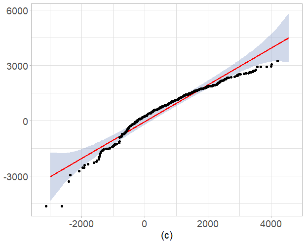
Finally, was generated using the Cauchy fields with , and and with . Note, that is a weakly dependent component while and are strongly dependent ones. The Q-Q plot analogous to Figure 5(b) presented in Figure 5(c) demonstrates that the distributions are different. The corresponding Kolmogorov-Smirnov -value is . In this case the asymptotic distribution of of strong-weak dependent components is non-Gaussian and is given by Theorem 5.
6 Conclusions
The paper obtains the reduction principle for vector random fields with strong-weak dependent components. In contrast to the known scalar and vector cases with same type memory components, it is shown that terms at levels do not necessarily determine limit behaviours. Applications to Minkowski functionals of Student random fields and numerical examples that illustrate the obtained theoretical results are presented. It would be interesting to extend the obtained results to the cases of
-
(1)
cross-correlated components by using some ideas from Theorems 10 and 11 in Leonenko and Olenko (2014). In these theorems it was assumed that the cross-correlation of components is given by some positive definite matrix Then, by using the transformation it was possible to transform the vector field to the one with non-correlated components;
-
(2)
. It is expected that under some additional assumptions these cases will lead to the CLT, see Remark 2.4 in Bai and Taqqu (2018);
-
(3)
non-central limit theorems where the condition is not satisfied. Obtaining such analogous of Theorems 4 and 5, it requires an extension of Arcones-Major results, see Arcones (1994); Major (2019), to continuous settings. While the direct proof may need substantial efforts, see Major (2019), one can try the simpler strategy proposed in Alodat and Olenko (2019). Namely, to prove that discrete and continuous functionals have same limits and then to apply the known discrete result from Arcones (1994) and Major (2019);
- (4)
Acknowledgements
Andriy Olenko was partially supported under the Australian Research Council’s Discovery Projects funding scheme (project DP160101366). The authors also would like to thank the anonymous referees for their suggestions that helped to improve the paper.
References
- Adler and Taylor (2009) Adler, R. and Taylor, J. (2009). Random Fields and Geometry. Milan: Springer.
- Alodat and Olenko (2019) Alodat, T. and Olenko, A. (2019). Asymptotic behaviour of discretised functionals of long-range dependent functional data. arXiv preprint. Available at \urlarXiv:1905.10030.
- Amiri et al. (2019) Amiri, M., Gómez, H. W., Jamalizadeh, A. and Towhidi, M. (2019). Bimodal extension based on the skew-t-normal distribution. Brazilian Journal of Probability and Statistics, 33(1), 2–23.
- Anh et al. (2015) Anh, V., Leonenko, N. and Olenko, A. (2015). On the rate of convergence to Rosenblatt-type distribution. Journal of Mathematical Analysis and Applications, 425(1), 111–132.
- Arcones (1994) Arcones, M. (1994). Limit theorems for nonlinear functionals of a stationary Gaussian sequence of vectors. The Annals of Probability, 22(4), 2242–2274.
- Arellano-Valle and Genton (2005) Arellano-Valle, R. B., and Genton, M. G. (2005). On fundamental skew distributions. Journal of Multivariate Analysis, 96(1), 93–116.
- Azzalini and Capitanio (2014) Azzalini, A. and Capitanio, A. (2014). The Skew-Normal and Related Families. New York: Cambridge University Press.
- Bai and Taqqu (2013) Bai, S. and Taqqu, M. (2013). Multivariate limit theorems in the context of long-range dependence. Journal of Time Series Analysis, 34(6), 717–743.
- Bai and Taqqu (2018) Bai, S. and Taqqu, M. (2018). How the instability of ranks under long memory affects large-sample inference. Statistical Science, 33(1), 96–116.
- Beran et al. (2013) Beran, J., Feng, Y., Ghosh, S. and Kulik, R. (2013). Long-Memory Processes: Probabilistic Properties and Statistical Methods. Heidelberg: Springer.
- Bingham et al. (1989) Bingham, N., Goldie, C. and Teugels, J. (1989). Regular Variation. Cambridge: Cambridge University Press.
- Breuer and Major (1983) Breuer, P. and Major, P. (1983). Central limit theorems for non-linear functionals of Gaussian fields. Journal of Multivariate Analysis, 13(3), 425–441.
- Bulinski et al. (2012) Bulinski, A., Spodarev, E. and Timmermann, F. (2012). Central limit theorems for the excursion set volumes of weakly dependent random fields. Bernoulli, 18(1), 100–118.
- Chambers and Slud (1989) Chambers, D. and Slud, E. (1989). Central limit theorems for nonlinear functionals of stationary Gaussian processes. Probability Theory and Related Fields, 80(3), 323–346.
- Coulon-Prieur and Doukhan (2000) Coulon-Prieur, C. and Doukhan, P. (2000). A triangular central limit theorem under a new weak dependence condition. Statistics and Probability Letters, 47(1), 61–68.
- de Naranjo (1995) de Naranjo, M. (1995). A central limit theorem for non-linear functionals of stationary Gaussian vector processes. Statistics and Probability Letters, 22(3), 223–230.
- Demichev (2015) Demichev, V. (2015). Functional central limit theorem for excursion set volumes of quasi-associated random fields. Journal of Mathematical Sciences, 204(1), 69–77.
- Dobrushin and Major (1979) Dobrushin, R. and Major, P. (1979). Non-central limit theorems for non-linear functional of Gaussian fields. Zeitschrift für Wahrscheinlichkeitstheorie und Verwandte Gebiete, 50(1), 27–52.
- Doukhan and Louhichi (1999) Doukhan, P. and Louhichi, S. (1999). A new weak dependence condition and applications to moment inequalities. Stochastic Processes and their Applications, 84(2), 313–342.
- Doukhan et al. (2002) Doukhan, P., Oppenheim, G. and Taqqu, M. (2002). Theory and Applications of Long-Range Dependence. Boston: Birkhäuser.
- Gihman and Skorokhod (2004) Gihman, I.I, and Skorokhod, A.V. (2004). The Theory of Stochastic Processes I. Berlin: Springer.
- Gneiting and Schlather (2004) Gneiting, T., and Schlather, M. (2004). Stochastic models that separate fractal dimension and the Hurst effect. SIAM Review, 46(2), 269–282.
- Hariz (2002) Hariz, S. (2002). Limit theorems for the non-linear functional of stationary Gaussian processes. Journal of Multivariate Analysis, 80(2), 191–216.
- Ivanov and Leonenko (1989) Ivanov, A. and Leonenko, N. (1989). Statistical Analysis of Random Fields. Dordrecht: Kluwer Academic.
- Klykavka et al. (2012) Klykavka, B., Olenko, A. and Vicendese, M. (2012). Asymptotic behavior of functionals of cyclic long-range dependent random fields. Journal of Mathematical Sciences, 187(1), 35–48.
- Kratz and Vadlamani (2018) Kratz, M. and Vadlamani, S. (2018). Central limit theorem for Lipschitz–Killing curvatures of excursion sets of Gaussian random fields. Journal of Theoretical Probability, 31(3), 1729–1758.
- Leonenko (1999) Leonenko, N. (1989). Limit Theorems for Random Fields with Singular Spectrum. Dordrecht: Kluwer Academic.
- Leonenko and Olenko (2013) Leonenko, N. and Olenko, A. (2013). Tauberian and Abelian theorems for long-range dependent random fields. Methodology and Computing in Applied Probability, 15(4), 715–742.
- Leonenko and Olenko (2014) Leonenko, N. and Olenko, A. (2014). Sojourn measures of Student and Fisher–Snedecor random fields. Bernoulli, 20(3), 1454–1483.
- Major (2019) Major, P. (2019). Non-central limit theorem for non-linear functionals of vector valued Gaussian stationary random fields. arXiv preprint. Available at \urlarXiv:1901.04086.
- Olenko (2013) Olenko, A. (2013). Limit theorems for weighted functionals of cyclical long-range dependent random fields. Stochastic Analysis and Applications, 31(2), 199–213.
- Olenko and Omari (2019) Olenko, A. and Omari, D. (2019). Reduction principle for functionals of vector random fields To appear in Methodology and Computing in Applied Probability. Available at \urlarXiv:1803.11271.
- Rosenblatt (1961) Rosenblatt, M. (1961). Independence and dependence. In Proceedings of the Fourth Berkeley Symposium on Mathematical Statistics and Probability. 2 (J. Neyman, eds.) 431–443, University of California Press, Berkeley.
- Schlather et al. (2019) Schlather, M., Malinowski, A., Oesting, M., Boecker, D., Strokorb, K., Engelke, S., Martini, J., Ballani, F., Moreva, O., Auel, J., Menck, P. J., Gross, S., Ober, U., Berreth, C., Burmeister, K., Manitz, J., Ribeiro, P., Singleton, R., Pfaff, B., and R Core Team (2019) RandomFields: Simulation and Analysis of Random Fields, R package version 3.3.6 \urlhttps://cran.r-project.org/package=RandomFields.
- Seneta (1976) Seneta, E. (1976). Regularly Varying Functions. Berlin: Springer.
- Souza (2008) Souza, L. R. (2008). Spectral properties of temporally aggregated long memory processes. Brazilian Journal of Probability and Statistics, 22(2), 135–155.
- Spodarev (2014) Spodarev, E. (2014). Limit theorems for excursion sets of stationary random fields. In Modern Stochastics and Applications, 90, 221–241. Cham : Springer.
- Taqqu (1975) Taqqu, M. (1975). Weak convergence to fractional Brownian motion and to the Rosenblatt process. Zeitschrift für Wahrscheinlichkeitstheorie und Verwandte Gebiete, 31(4), 287–302.
- Taqqu (1977) Taqqu, M. (1977). Law of the Iterated logarithm for sums of non-linear functions of Gaussian variables that exhibit a long range dependence. Zeitschrift für Wahrscheinlichkeitstheorie und Verwandte Gebiete, 40, 203–238.
- Taqqu (1979) Taqqu, M. (1979). Convergence of integrated processes of arbitrary Hermite rank. Zeitschrift für Wahrscheinlichkeitstheorie und Verwandte Gebiete, 50(1), 53–83.
- Worsley (1994) Worsley, K. (1994). Local maxima and the expected Euler characteristic of excursion sets of , F and t fields. Advances in Applied Probability, 26(1), 13–42.