Redundancy analysis using lcm-filtrations: networks, system signature and sensitivity evaluation

The structure of least common multiples of sets of minimal generators of monomial ideals is a key combinatorial tool both in the study of these ideals [12, 19, 6, 18] and in their applications. Computing this structure is a computationally demanding task, and it sometimes introduces redundancy that is undesirable in certain situations, particularly when it leads to the expenditure of computing resources on meaningless computations. Some applications of monomial ideals in which their lcm-structure is useful include the analysis of simultaneous failures in coherent systems [23], multivariate signature analysis [26], and sensitivity analysis of preference functions [9].

In all of these applications (and their computational aspects), the lcm-filtration was used. The redundancy introduced by this filtration is, in these cases, both a feature and an issue. In this paper, we introduce the stepwise lcm-filtration as a way to handle the least common multiple structure of sets of generators of monomial ideals. This approach can be faster and less redundant but sometimes coarser than the usual lcm-filtration (see Section 2). Subsequently, we dedicate the rest of the sections to analysing the conditions, in various applications, under which redundancy provides meaningful information and those under which non-redundant computations are more useful or feasible.

Section 3 focuses on cut ideals of graphs, as used in network theory [17]. We demonstrate that the proposed stepwise filtration exhibits favourable properties in the analysis of sparse networks and graphs, and we describe a phase transition for random graphs concerning the behaviour of the redundancy in the lcm-structure of their corresponding cut ideals. Another application of these ideas pertains to $k$-out-of-$n$ systems and their significant variants: linear and circular consecutive $k$-out-of-$n$ systems. In Section 4, we show that their behaviour with respect to redundancy differs, making the combined use of the stepwise lcm-filtration and the usual one both useful and convenient for the optimal treatment of these systems.

Finally, Section 5 addresses sensitivity analysis, where the stepwise filtration and the usual lcm-filtration complement each other in two ways. First, on a global analysis of the sensitivity of a model, the stepwise filtration avoids processing equal steps in the filtration when such information is unnecessary and also offers a direct interpretation of the filtration steps in a simplicial formulation, enhancing the understanding of factor interactions in simplicial terms. Second, focusing in the local features at each sensitive corner, the redundancy provided by the usual lcm-filtration is better suited to analyse the differences among complexes having the same f-vector and Betti numbers by means of distances between persistence diagrams associated to these filtrations.

Let $G$ be a graph with the vertex set $V=\{1,\ldots,i\}$ and the edge set $E$. For a $j$-partition $C=A_{1}|A_{2}|\ldots|A_{j}$ of $V$, consisting of $j$ disjoint nonempty subsets $A_{k}\subset V$ we define

A $j$-partition $C=A_{1}|A_{2}|\ldots|A_{j}$ of the set $\{1,\dots,i\}$ is called a $j$-cut of a graph $G$ if the subgraph induced by each part $A_{k}$ ($1\leq k\leq j$) is connected. Let $\mathcal{P}_{i,j}(G)$ denote the set of $j$-partitions of $G$.

Let $\mathbf{k}$ be a field, and let $R=\mathbf{k}[x_{e}:e\in E]$ denote the polynomial ring in the variables corresponding to the edges of $G$. We associate the monomial

to each cut $C=A_{1}|A_{2}|\ldots|A_{j}$ of $G$. The cut ideal $\mathcal{C}_{G}$ of $G$ is the ideal in $R$ generated by all $m_{C}$ for $2$-cuts $C$ of $G$. Let $P_{i,j}$ denote the ideal minimally generated by the monomials $m_{C}$, where $C$ is a $j$-partition in $\mathcal{P}_{i,j}(G)$. In words, the ideal $P_{i,j}$ has a minimal generator corresponding to each $j$-partition $C$ in $\mathcal{P}_{i,j}(G)$.

We now focus on two extreme families of graphs: complete graphs and trees. In Section 3.1, we will study the transition between these two extreme cases on random graphs.

First, we describe the simplicial complexes in the lcm-filtration of the cut ideals of complete graphs as follows. The result follows directly from the definition, and therefore, we omit the proof.

Consider the complete graph $K_{i}$ with the vertex set $[i]$. For each $j$ with $1\leq j\leq i$, we denote the $j$-fold $\operatorname{lcm}$-ideal of $I$ with $I_{i,j}$. We have the following relations between the ideals $I_{i,j}$ and the ideals $P_{i,j}$ which gives a nice combinatorial description of the lcm-ideals of the cut ideal of the complete graph $K_{i}$.

Before stating the main result, we recall that the Stirling number of the second kind, denoted by $S(n,k)$, represents the number of ways to partition a set of $n$ elements into $k$ non-empty, disjoint subsets.

The following tables records the number of generators of the ideals $P_{i,j}$, the ideal of the $j$-cuts of $K_{i}$. for $i$ and $j$ up to $10$.

As an immediate consequence of the above theorem we have:

Let us now consider the graph $G=T_{i}$, a tree on the vertex set $\{1,\ldots,i\}$. The number of edges in $T_{i}$ is $i-1$, and each edge is a $2$-cut for $T_{i}$. The ideal $P_{i,2}$ is generated by all the variables, so it has a Taylor lattice, indicating that there is no redundancy in the lattice structure of these ideals, unlike in the case of complete graphs. Furthermore, since $T_{i}$ has no cycles, any set of $j$ edges of $T_{i}$ forms a $j$-cut. Hence, we have the following corollary:

We conclude by noting that cut ideals naturally arise in the context of divisor theory (see, for example, [29, 25, 24, 20]), and that their Betti numbers and resolutions have been extensively studied.

In the fields of systems reliability and signature analysis [33, 3, 13], the lcm structure of the associated ideals is fundamental for analyzing simultaneous events. As highlighted in [22, 23, 26], a pivotal step in studying simultaneous failures in a system involves computing the various $k$-fold lcm-ideals of its associated failure ideal $I$.

Let $n$ be a positive integer, and let $S$ be a coherent system with $n$ components, each taking one of finitely many possible states. The states of the system can be represented as elements of $\mathbb{N}^{n}$, with a designated subset of failure states $F$, assumed to be coherent (i.e., closed under entrywise ordering). These failure states correspond to the exponents of the monomials in the failure ideal $I$ within $\mathbf{k}[\mathbf{x}]:=\mathbf{k}[x_{1},\dots,x_{n}]$.

Suppose minimal failures can occur simultaneously in the system, and let $Y$ represent the number of such simultaneous failures. The event $\{Y\geq 1\}$ corresponds to system failure, while the intersection of two failure events, $\mathbf{x}^{\alpha}$ and $\mathbf{x}^{\beta}$, results in $\operatorname{lcm}(\mathbf{x}^{\alpha},\mathbf{x}^{\beta})=\mathbf{x}^{\alpha\lor\beta}$, representing the event $\{Y\geq 2\}$. This reasoning naturally extends to $\{Y\geq k\}$, enabling the study of tail probabilities $\operatorname{Prob}(Y\geq k)$. Hence, simultaneous failures are encoded within the $k$-fold lcm-ideals $I_{k}$. Finally, consider a probability distribution defined over the system’s states. The system’s reliability is the probability that it remains in a working state, while its unreliability (or failure probability) is given by $\mathbb{E}[1_{F}]$, the expected value of the indicator function of the failure set $F$.

In a system with $n$ components that fail independently according to a common failure time distribution and density, the order statistics of the failure times are denoted as $T_{(1)},T_{(2)},\dots,T_{(n)}$. The system fails at time $T=T_{(i)}$ for some $i\in\{1,\dots,n\}$, with probabilities:

These probabilities, $s_{1},\dots,s_{n}$, can be computed using the failure ideal $I$ and its squarefree representation. Here, $s_{i}$ represents the conditional probability that exactly $i$ components have failed, given that the system has failed. If $P_{i}$ denotes the probability of exactly $i$ components failing, then $s_{i}=\frac{P_{i}}{P(F)}$, where $P(F)$ is the total failure probability. Alternatively, $s_{i}$ can be expressed as:

where $E_{i}$ is the set of failure states corresponding to exactly $i$ failed components.

For the case of multiple simultaneous failures, we define $T_{k}^{(i)}$ as the time of the $k$-th minimal failure, given that $i$ components fail. The $k$-fold signature $s_{k}^{i}$ represents the associated probabilities:

Let $I$ be the failure ideal of the system, and let $I_{k}$ denote the $k$-fold lcm-ideal of $I$. The $k$-fold lcm-ideal $I_{k}$ encodes the system states where at least $k$ failures occur simultaneously. We define $I^{[i]}_{k}$ to be the ideal generated by the squarefree monomials of degree $i$ in $I_{k}$. The $k$-fold signature $s_{k}^{i}$ is determined as the difference of the Hilbert series evaluations of the ideals $I_{k}^{[i]}$ and $I_{k}^{[i+1]}$:

where $H(\cdot)$ denotes the Hilbert series. This formulation captures the relationship between the algebraic invariants of the lcm-ideals and the probabilities of simultaneous failures in coherent systems.

In general, the study of simultaneous failure and signature involves the study of $lcm$-filtrations of the corresponding ideals. This might be in general computationally demanding and therefore, under some circumstances, the study of the stepwise filtration is a viable alternative, recall Section 2.5. In the rest of this section we make this observation explicit for one of the most important families of coherent systems, namely $k$-out-of-$n$ systems and variants.

One of the key models in applied reliability engineering is the $k$-out-of-$n$:F system, where F denotes failure [16]. In such a system, failure occurs whenever at least $k$ out of $n$ components fail. A variation, the consecutive linear $k$-out-of-$n$ model, fails whenever $k$ consecutive components fail. The analysis of simultaneous failures in these systems is crucial for many applications [1, 26, 35].

The number of minimal failure events in these systems grows exponentially with respect to the number of minimal failures of the system itself. Generally, when $k\ll n$, these systems exhibit low redundancy. However, for the consecutive $k$-out-of-$n$ model, as observed in [26], this low redundancy makes the problem computationally demanding when using the usual $k$-fold lcm ideal filtration for computation. In some cases, this computation may even exceed the cost of calculating the system’s reliability.

One way to address this challenge is to derive explicit formulas for the generators of these systems, as demonstrated in [23, 26]. However, these techniques are not easily adaptable to other types of systems. To overcome this limitation, we analyze the redundant and non-redundant regimes introduced in Section 3.1 and apply this framework also to circular consecutive $k$-out-of-$n$:F systems [30, 16], which cannot be efficiently studied using the approaches from [26].

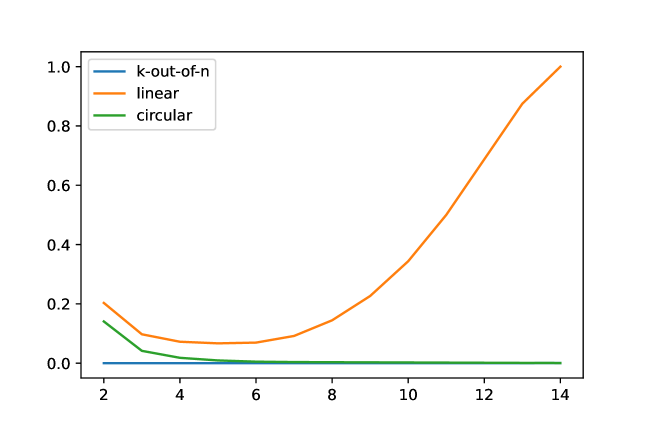
Figure 2 illustrates the behavior of three types of systems, namely $k$-out-of-$n$, consecutive linear $k$-out-of-$n$, and consecutive circular $k$-out-of-$n$ for $n=15$ and $k=2,\dots,9$. The $k$-out-of-$n$ systems are characterized by $\binom{n}{k}$ generators with a high degree of overlap, resulting in a very low ratio between the size of the full poset on those generators and the size of the lcm-lattice of the ideal. This makes the usual lcm-filtration impractical for large values of $n$.

In contrast, consecutive $k$-out-of-$n$ systems have fewer generators, leading to smaller total posets. For these systems, the ratio of the full poset size to the actual lcm-lattice size favors the stepwise version of the lcm-filtration when the overlap is moderate. However, for cases of very high or very low overlap, the usual lcm-filtration proves more efficient.

Lastly, the consecutive circular model has a constant number of generators, specifically $n$ generators, for all values of $k$. As the overlap, determined by $k$, increases, the ratio decreases. In this case, the stepwise lcm-filtration is the optimal choice, particularly since there are no known formulas, as in [26], for the number of generators and Betti numbers of common failure ideals in these systems.

Sensitivity analysis of models studies how different sources of uncertainty in the model inputs influence the uncertainty in the output. It is commonly applied in exploratory modeling, model evaluation, simplification, or refinement. In [9], the authors considered a multi-factor binary decision-making system, and analyzed such systems using an algebraic-combinatorial approach. Monomial ideals and their associated simplicial complexes, were used to identify the input combinations most critical to the decision and warranting careful review. These key combinations were found as the multidegrees at which the ideal representing the system has non-zero Betti numbers, referred to as sensitive corners of the model. To investigate the variations in the effects of different factor combinations, we analyzed the persistence homology [4] of the simplicial complexes at each sensitive corner, using the standard lcm-filtration. The method presented in [9] can be enhanced by using stepwise lcm-filtration in at least two ways. First, the correspondence between ideals and simplicial complexes in the filtration, outlined in Theorem 2.4, facilitates the interpretation of factor interactions as simplicial complexes. Second, as observed in the signature analysis (Section 4), there is redundancy in the process, where certain simplicial complexes remain unchanged throughout the filtration. While the usual lcm-filtration does not handle this redundancy, the stepwise version efficiently manages it.

Consider a decision system that makes a binary decision based on the satisfaction levels of $n$ factors. The minimum acceptance points of the system are the combinations of factor scores such that any decrease in the satisfaction level of any factor leads to rejection. Let the polynomial ring be $\mathbf{k}[\mathbf{x}]:=\mathbf{k}[x_{1},\dots,x_{n}]$. For this system $S$, we associate a monomial ideal $I_{S}\subseteq\mathbf{k}[\mathbf{x}]$, where each variable represents one factor. Each minimal generating monomial of $I_{S}$ corresponds to a minimal acceptance point of $S$. The multidegrees of $I_{S}$ at which interactions between minimal acceptance points occur (elements of the lcm-lattice of $I_{S}$) are referred to as the sensitivity corners of the system or model. At each of these sensitivity corners, with multidegree $\mu$, we can construct a local simplicial complex that models the multi-factor interactions.

The relationship between the Betti numbers of $I_{S}$ at $\mu$ and those of the corresponding Koszul simplicial complexes is given by the well-known Hochster’s formula.

We can now apply these tools to perform sensitivity analysis at each corner, either from an ideal-based or simplicial-based perspective. The ideal-based approach is typically more suited for computations, while the simplicial-based approach is better for interpreting the results.

In [9], the primary tool used is persistent homology of the simplicial complexes at the sensitive corners, based on the usual lcm-filtration. The main idea is the following: At each corner of the system ideal, we analyze the Koszul simplicial complex using the lcm or stepwise-lcm filtration of the ideal of the system. Based on this, we cluster these corners to perform a detailed analysis. The analysis in [9] (see Section 5 there) shows that this clustering groups the complexes based on size related features, such as number of vertices or number of simplices. This analysis based on the system ideal measures the local effect (at each corner) of interactions between the factors of the minimal acceptance points. In this case, the stepwise filtration offers an efficient alternative to the usual lcm one. However, to distinguish the behaviour of the corners within each cluster, a more detailed local analysis is needed. This can be done by means of the persistence homology of the local simplicial complexes themselves, and in this case, the lcm filtration is advantageous, since it amplifies the distances between persistence diagrams with respect to those obtained . The following example illustrates this idea.

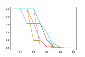
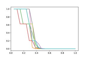
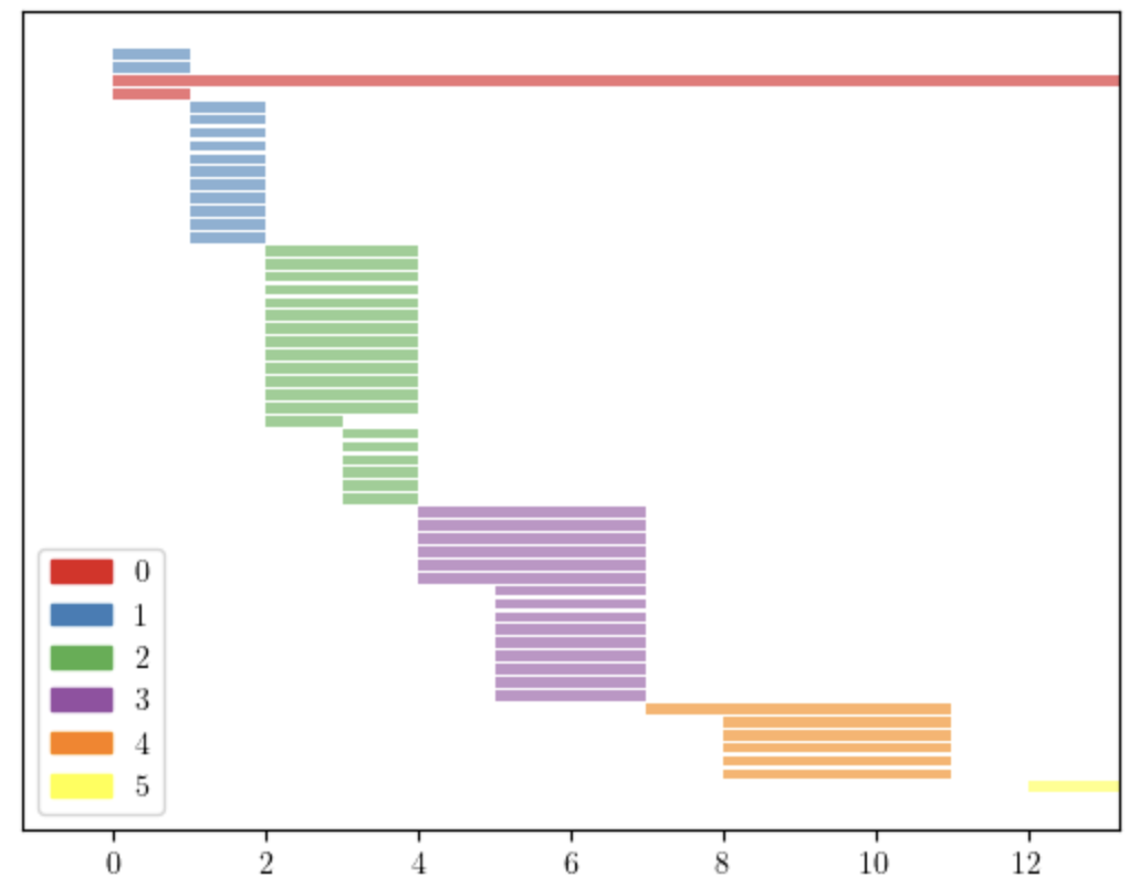
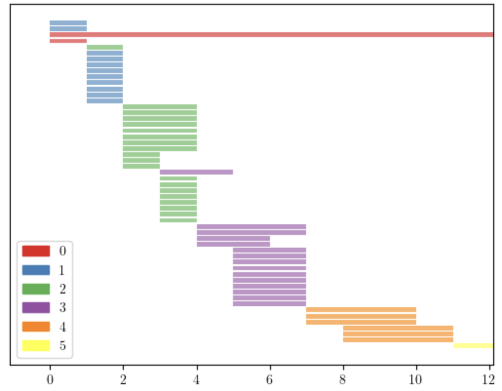
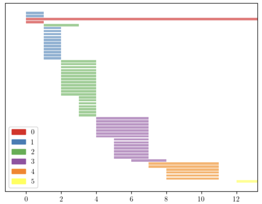
Consider the complexes in Figure 3, which have the same f-vector: $(1,7,7)$ and same Betti numbers: $\beta_{0}=2$, $\beta_{1}=2)$. We apply the lcm filtration to them and obtain the persistence diagrams in Figure 4. Applying the stepwise filtration we obtain the diagrams in Figure 5, which are much shorter and similar to each other. This can be observed using the distance between persistence diagrams. Tables 1 and 2 show the Bottleneck and Wasserstein distances [7, 10] between the persistence diagrams of the four complexes in Figure 3. We can see the amplification effect of the lcm-filtration, which is more evident when we use the Wasserstein distance.

In this paper, we introduced two tools for analyzing the least common multiple (lcm) structure of monomial ideals: the lcm-filtration and the stepwise filtration. Both filtrations provide information about the structure of these ideals, as well as the associated simplicial complexes, with broad applicability in various contexts. Specifically, we have explained their use in cut ideals of graphs, simultaneous failures in coherent systems, and sensitivity analysis. In each case, these filtrations allowed us to study the balance between redundancy, efficiency, and information. The tools and applications presented open several avenues for future research on the application of monomial ideals and simplicial complexes in various fields contexts.

The research is partially supported by the project INICIA2023/02 funded by La Rioja Government (Spain), as well as the KU Leuven grant iBOF/23/064, and the FWO grants G0F5921N and G023721N.

References

- [1] K. Adachi, M. Kodama, and M. Ohashi. k-out-of-n: G system with simultaneous failure and three repair policies. Microelectronics Reliability, 19(4):351–361, 1979.
- [2] G. Alesandroni. Minimal resolutions of dominant and semidominant ideals. Journal of Pure and Applied Algebra, 221(4):780–798, 2017.
- [3] P. J. Boland. Signatures of indirect majority systems. Journal of applied probability, 38(2):597–603, 2001.
- [4] G. Carlsson and A. Zomorodian. Computing persistent homology. Discrete and Computational Geometry, 33(2):249–274, 2005.
- [5] R.-X. Chen. Lcm-lattice, taylor bases and minimal free resolutions of a monomial ideal. Journal of Algebra and Its Applications, 21(11):2250216, 2022.
- [6] T. B. Clark. Poset resolutions and lattice-linear monomial ideals. Journal of Algebra, 323(4):899–919, 2010.
- [7] D. Cohen-Steiner, H. Edelsbrunner, and J. Harer. Stability of persistence diagrams. Discrete and Computational Geometry, 37(1):1103–120, 2007.
- [8] J. A. De Loera, S. Petrović, L. Silverstein, D. Stasi, and D. Wilburne. Random monomial ideals. Journal of Algebra, 519:440–473, 2019.
- [9] J. Divasón, F. Mohammadi, E. Sáenz-de-Cabezón, and H. Wynn. Sensitivity analysis of discrete preference functions using Koszul simplicial complexes. In Proceedings of the 2023 International Symposium on Symbolic and Algebraic Computation, pages 227–235, 2023.
- [10] H. Edelsbrunner and J. Harer. Computational topology: an introduction. American Mathematical Society, 2010.
- [11] P. Erdős and A. Rényi. On random graphs. i. Publicationes Mathematicae, 6(3-4):290–297, 1959.
- [12] V. Gasharov, I. Peeva, and V. Welker. The lcm-lattice in monomial resolutions. Mathematical Research Letters, 6:521–532, 1999.
- [13] A. K. Goharshady and F. Mohammadi. An efficient algorithm for computing network reliability in small treewidth. Reliability Engineering & System Safety, 193:106665, 2020.
- [14] J. Herzog and T. Hibi. Monomial ideals. Springer, 2011.
- [15] M. Hochster. Cohen-Macaulay rings, combinatorics, and simplicial complexes, in ring theory ii. Lect. Notes in Pure Appl. Math., (26):171–223, 1977.
- [16] W. Kuo and M. Zuo. Optimal reliability modelling. John Wiley and sons, 2002.
- [17] Q. Liu, Z. Dong, and E. Wang. Cut based method for comparing complex networks. Scientific reports, 8(1):5134, 2018.
- [18] S. Mapes. Finite atomic lattices and resolutions of monomial ideals. Journal of Algebra, 379:259–276, 2013.
- [19] E. Miller and B. Sturmfels. Combinatorial commutative algebra. Springer, 2005.
- [20] F. Mohammadi. Divisors on graphs, orientations, syzygies, and system reliability. Journal of Algebraic Combinatorics, 43:465–483, 2016.
- [21] F. Mohammadi, P. Pascual-Ortigosa, E. Sáenz-de Cabezón, and H. P. Wynn. Polarization and depolarization of monomial ideals with application to multi-state system reliability. Journal of Algebraic Combinatorics, 51(4):617–639, 2020.
- [22] F. Mohammadi, E. Sáenz-de Cabezón, and H. P. Wynn. The algebraic method in tree percolation. SIAM Journal on Discrete Mathematics, 30(2):1193–1212, 2016.
- [23] F. Mohammadi, E. Sáenz-de-Cabezón, and H. P. Wynn. Types of signature analysis in reliability based on Hilbert series. Journal of Symbolic Computation, 79(1):140–155, 2017.
- [24] F. Mohammadi and F. Shokrieh. Divisors on graphs, connected flags, and syzygies. International Mathematics Research Notices, 2014(24):6839–6905, 2014.
- [25] F. Mohammadi and F. Shokrieh. Divisors on graphs, binomial and monomial ideals, and cellular resolutions. Mathematische Zeitschrift, 283(1):59–102, 2016.
- [26] F. Mohammadi, E. Sáenz-de-Cabezón, and H. P. Wynn. Efficient multicut enumeration of k-out-of-n:f and consecutive k-out-of-n:f systems. Pattern Recognition Letters, 102:82 – 88, 2018.
- [27] M. Newman. Networks. An Introduction. Oxford University Press, 2010.
- [28] J. Phan. Order properties of monomial ideals and their free resolutions. PhD thesis, Columbia University, 2006.
- [29] A. Postnikov and B. Shapiro. Trees, parking functions, syzygies, and deformations of monomial ideals. Transactions of the American mathematical society, 356(8):3109–3142, 2004.
- [30] W. W. Preuss and T. K. Boehme. On Reliability Analysis of Consecutive-k Out-Of-n: F Systems and Their Generalizations — A Survey, pages 401–411. Springer US, Boston, MA, 1994.
- [31] E. Sáenz-de-Cabezón and H. P. Wynn. Betti numbers and minimal free resolutions for multi-state system reliability bounds. Journal of Symbolic Computation, 44:1311–1325, 2009.
- [32] E. Sáenz-de-Cabezón and H. P. Wynn. Hilbert functions for design in reliability. IEEE Trans. Rel., 64:83–93, 2015.
- [33] F. J. Samaniego. System signatures and their applications in engineering reliability, volume 110. Springer Science & Business Media, 2007.
- [34] D. K. Taylor. Ideals generated by monomials in an R-sequence. Phd thesis, University of Chicago, 1966.
- [35] T. Yuge. Reliability of systems with simultaneous and consecutive failures. In 2019 4th International Conference on System Reliability and Safety (ICSRS), pages 102–106, 2019.