Refiner: Data Refining against Gradient Leakage Attacks in Federated Learning
Abstract
Recent works have brought attention to the vulnerability of Federated Learning (FL) systems to gradient leakage attacks. Such attacks exploit clients’ uploaded gradients to reconstruct their sensitive data, thereby compromising the privacy protection capability of FL. In response, various defense mechanisms have been proposed to mitigate this threat by manipulating the uploaded gradients. Unfortunately, empirical evaluations have demonstrated limited resilience of these defenses against sophisticated attacks, indicating an urgent need for more effective defenses. In this paper, we explore a novel defensive paradigm that departs from conventional gradient perturbation approaches and instead focuses on the construction of robust data. Intuitively, if robust data exhibits low semantic similarity with clients’ raw data, the gradients associated with robust data can effectively obfuscate attackers. To this end, we design Refiner that jointly optimizes two metrics for privacy protection and performance maintenance. The utility metric is designed to promote consistency between the gradients of key parameters associated with robust data and those derived from clients’ data, thus maintaining model performance. Furthermore, the privacy metric guides the generation of robust data towards enlarging the semantic gap with clients’ data. Theoretical analysis supports the effectiveness of Refiner, and empirical evaluations on multiple benchmark datasets demonstrate the superior defense effectiveness of Refiner at defending against state-of-the-art attacks.
1 Introduction
The past decade has witnessed a remarkable surge in the demand for extensive datasets [36, 38, 32], which serve as the driving force behind the recent astonishing breakthroughs achieved by deep neural networks (DNNs) across diverse domains [9, 11, 29]. However, the acquisition of large-scale datasets presents significant challenges. Entities and organizations are often reluctant to share their internal data due to concerns about potential leakage of sensitive information [23]. A notable example is the healthcare sector [42, 31], which is bound by privacy protection laws that strictly prohibit the sharing of patient-related information. Thus, training DNNs while safeguarding privacy has become a fundamental problem.
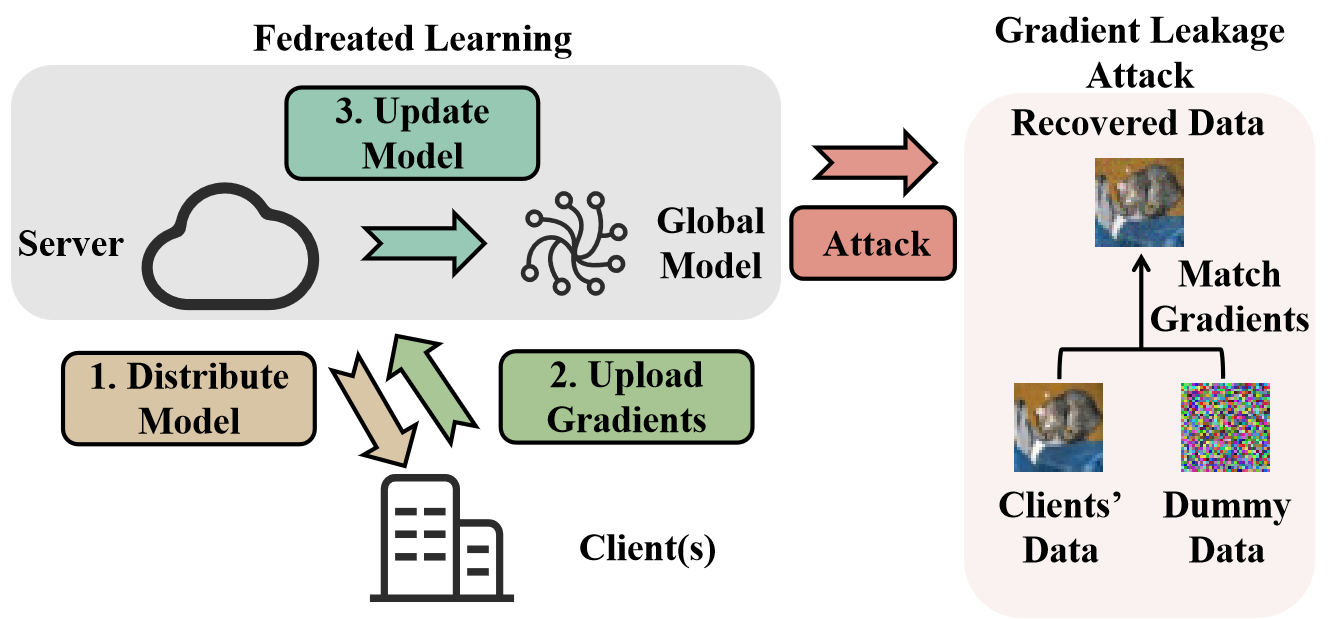
To address the abovementioned problem, Federated Learning (FL) has emerged as a highly promising privacy-preserving training framework [23]. In FL, as depicted in Figure 1, multiple clients participate by computing gradients locally [27], which are then contributed to a global server. The global server aggregates the uploaded gradients to update a globally-shared model, subsequently distributing the updated model back to the participating clients for the next training round. This collaborative process ensures that the privacy of individual client data is preserved, as the communication is limited to gradients or model parameters rather than the raw data itself. The prevailing belief in the practicability and effectiveness of FL has led to its widespread adoption across various privacy-sensitive scenarios. However, recent works on Gradient Leakage Attacks (GLAs) [54, 53, 12, 48] have challenged this belief by demonstrating that gradients alone are sufficient to reconstruct clients’ raw data. As shown in Figure 1, these attacks align the gradients of model parameters associated with dummy data with uploaded gradients and exploit the optimization process of the dummy data to closely resemble the original client data, thereby reconstructing sensitive information with a high level of fidelity. GLAs highlight the need for effective defenses in FL to ensure the confidentiality of sensitive client information.
Two primary types of methods have been proposed to safeguard privacy in FL: encryption-based methods [28, 8, 50, 10, 5] and perturbation-based methods [1, 54, 52, 39, 44]. Encryption-based methods ensure that the server only obtains encrypted versions of clients’ uploaded gradients, thereby enhancing privacy protection. However, the aggregated gradients still need to be decrypted into plaintext [10, 5], making them still vulnerable to GLAs. Moreover, encryption-based methods introduce considerable computational costs, data storage, and communication overheads which dominate the training process, thus significantly affecting the practicability of such methods [54, 39, 44, 50].
Perturbation-based methods typically impose subtle perturbation into ground-truth gradients, which helps to obscure the adversary’s (the server’s) ability to recover accurate data from the gradients. However, perturbation-based methods inherently involve a trade-off between utility (model performance) and privacy. Notable defenses include differential privacy [1] and gradient pruning [2], which perturb gradients by injecting random noises or discarding part of gradients. Recent research [46, 52] has revealed that gradient compression, specifically low-bit gradient quantization [4, 37, 34], can also contribute to defending against GLAs. State-of-the-art defenses [39, 44] estimate the privacy information contained in each gradient element for gradient pruning, theoretically achieving the optimal trade-off. Unfortunately, recent empirical evaluations [3, 49] have shown that these defenses struggle to achieve a satisfactory balance between privacy protection and model performance. In fact, these defenses often rely on oversimplified assumptions that do not align with the high complexity of DNNs (Section 7). As a result, it remains a challenge to craft appropriate perturbations for DNNs that effectively mislead the adversary while still providing informative gradients for the global model. Designing more effective defenses against GLAs remains to be explored.
In this paper, we explore a novel defensive paradigm that departs from conventional gradient perturbation approaches and instead focuses on the construction of robust data. Our inspiration stems from an intuitive yet compelling idea: if we can generate robust data that exhibit substantial significant semantic dissimilarity compared to clients’ raw data while maintaining utility, the gradients associated with these data are likely to have the potential to effectively obfuscate attackers while causing only minimal degradation in the model’s performance.
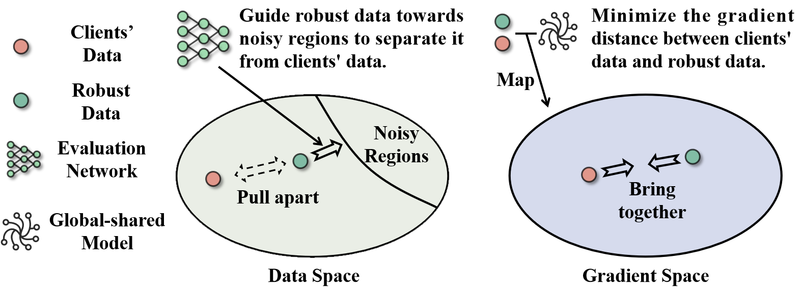
To realize this idea, we propose Refiner which crafts robust data by jointly optimizing two key metrics for privacy protection and performance maintenance. As illustrated in Figure 2, the privacy metric, i.e., the evaluation network, encourages robust data to deviate semantically from clients’ raw data, while the utility metric aligns the gradients of model parameters associated with clients’ data and robust data. In practice, to protect privacy, clients do not directly upload the gradients associated with their raw data. Instead, they upload gradients of robust data that are crafted through Refiner for their raw data, thereby maintaining the confidentiality of clients’ raw data.
-
•
Privacy metric. While norm-based distances between robust data and original data are commonly used to measure privacy [39], their effectiveness is limited due to the significant divergence with human-vision-system difference metrics [40]. To address this limitation, Refiner instead employs an evaluation network to accurately estimate the human perception distance between robust data and original data. The perception distance serves as the privacy metric, reflecting the overall amount of disclosed privacy information associated with clients’ data. By leveraging the human perception distance, Refiner provides a more accurate and effective evaluation of the privacy information contained in robust data.
-
•
Utility metric. The utility metric is defined as the weighted distance between the gradients of model parameters with respect to robust data and clients’ data. By minimizing the gradient distance, the utility of the robust data approaches that of the clients’ data. The weighting scheme prioritizes the preservation of gradients associated with important parameters, thus better maintaining the utility of the robust data. This weighting mechanism consists of element-wise weight and layer-wise weight. The element-wise weight is determined based on empirical and theoretical observations, considering the values of both gradients and parameters to identify critical parameters. Additionally, the layer-wise weight exploits the significance of earlier layers by allocating more attention to them during the learning process.
We also provide a solid theoretical foundation for these metrics and the effectiveness of Refiner and conduct extensive experiments on multiple benchmark datasets to show the superior performance of Refiner compared to baselines in defending against state-of-the-art attacks.
2 Background & Related Work
2.1 Federated Learning
Training DNNs while maintaining client privacy has become a crucial necessity due to data protection regulations111https://www.dlapiperdataprotection.com/, such as General Data Protection Regulation of the European Union. FL serves as a promising privacy-preserving solution through a gradient exchange mechanism between clients and a server [23]. We focus on a typical FL scenario, where a server collaborates with a set of clients to train a model parameterized by , utilizing loss function . The -th client’s local dataset is denoted by . The server and clients interact with each other for a total of rounds by alternately executing the two steps:
-
•
Model Distribution and Local Training. The server samples a subset of clients from the entire client pool to participate in the current round while the others await their turn. The server broadcasts the global model to selected clients. The -th selected client () samples raw data from his local dataset and computes gradients .
-
•
Global Aggregation. The server performs global aggregation by averaging the gradients received from selected clients, which are subsequently used to update the global model: where is the learning rate.
In the literature [27, 34], selected clients may update the local model over multiple steps and then upload the final model parameters. In this paper, we employ a default local step of 1, where clients directly upload the gradients without performing multiple local updates. The rationale behind this decision stems from the fact that the server typically derives gradients by comparing the global model parameters with the uploaded local model parameters. Multiple local steps could potentially lead to a discrepancy between the derived gradients and the ground-truth gradients associated with clients’ data, thereby reducing the effectiveness of attacks [52]. Thus, we adopt the setting that considers the most powerful attack scenario to better examine the effectiveness of defenses.
2.2 Threat Model
We assume that the server is honest-but-curious [44], which adheres to the pre-defined training rules but with a strong intention of recovering clients’ raw data by exploiting uploaded gradients. We allow the server to access public data sources and sufficient computational resources, thereby enabling the server to launch stronger attacks to evaluate our defense more thoroughly. We suppose that clients are aware of the privacy risks, and, as a remedy, clients proactively adopt defenses. To simplify the notations, subscripts, and superscripts representing specific clients are omitted throughout the paper.
2.3 Gradient Leakage Attack
The seminal work of GLAs was proposed by Zhu et al. [54]. Given randomly initialized dummy data with dummy label and uploaded gradients , the server tackles a gradient matching problem as follows:
| (1) |
Empirical evaluations illustrated the remarkable similarity between resulting and clients’ data . The Follow-up work [43, 53] showed how to infer the ground-truth label from the gradients of the fully-connected layer, reducing the complexity associated with solving Equation 1. However, several studies [46, 12, 48] empirically demonstrated that bad initialization causes convergence towards local optima, making recovered data noisy. In response, Geiping et al. [12] and Jeon et al. [20] dedicated efforts to explore various regularization techniques and heuristic tricks, including total variation, restart, and improved initialization, aiming to eliminate invalid reconstructions. Recently, since the output of generative models is not noisy, Li et al. [25] and Yue et al. [49] trained a generative network to recover clients’ data. The potential assumption is the availability of an abundance of data that is similar to the clients’ data. They optimized latent vectors of the generative network to produce images whose gradients are similar to uploaded ones.
2.4 Gradient Leakage Defense
While cryptographic methods have emerged as potential solutions in defending GLAs, the substantial overhead limits their applicability [54, 44, 25]. Similar to [54, 44, 25], this paper does not discuss cryptographic methods, but instead mainly investigates alternative perturbation-based methods [54, 3, 47]. One such perturbation-based method [54, 3, 47] is differential privacy (DP), which involves adding random noises to ground-truth gradients to generate perturbed gradients. Moreover, some work [39, 44] explored gradient pruning or gradient quantization (GQ) to obfuscate the server. Soteria, proposed by Sun et al. [39], employs a theoretically-derived metric to evaluate the privacy information contained in each gradient element and selectively prunes gradients in fully-connected layers. However, Balunović et al. [3], Wang et al. [44] discovered that Soteria could be compromised by muting gradients in fully-connected layers during the reconstruction process (Equation 1). To address this vulnerability, they developed a gradient mixing mechanism to solve the problem.
3 Our Approach: Refiner
3.1 Problem Formulation
We here formulate the problem that Refiner solves. The primary objective is to construct robust data that possess sufficient utility while minimizing the disclosure of privacy information from clients’ raw data . Then, Refiner upload gradients associated with . Refiner formulates the following optimization problem to craft robust data:
| (2) |
where and denote the utility and privacy metrics. evaluates the degree to which diverges from in terms of utility, while quantifies the reduction in privacy associated with compared to . serves as a balance factor to regulate the trade-off between utility and privacy. Increasing places a higher priority on privacy protection. Intuitively, with well-defined metrics, the optimal solution of Equation 2 aligns with our definition of robust data. Section 3.2 and Section 3.3 will elaborate on our and , respectively.
3.2 Utility Metric
3.2.1 Motivation
The utility of data is defined as the extent to which it contributes to reducing the model loss. DNNs utilize gradients to update model parameters to minimize loss, making it straightforward to exploit the mean square error (MSE) between gradients associated with and as the utility metric, i.e., . However, adopting the vanilla form of MSE treats all gradient elements equally. Consequently, minimizing the distance between gradient elements at different positions yields identical improvements in utility, disregarding the varying contributions of different parameters on model performance.
We customize a weighted MSE to more effectively evaluate the utility contained in . The overall idea of weighted MSE is to endow the gradients of important parameters with higher weights, so as to pay more attention to aligning the gradients of important parameters associated with and . To determine the weights, we consider two factors: element-wise weight along with layer-wise weight. The product of element-wise weight and layer-wise weight is used as the ultimate weight for the corresponding gradient element.
3.2.2 Element-wise Weight
Insight 1
The significance of parameters is closely tied to both their values and gradients. Intuitively, parameters with high magnitude values are crucial since they can considerably amplify their inputs. Higher outputs are more likely to exert a more substantial influence on the model’s predictions. Besides, the essence of gradient is quantifying the impact of a slight modification in parameters on the loss [6]. Hence, parameters that own gradients with larger magnitudes yield a greater influence in shaping the model performance.
Based on Insight 1, the element-wise weight can be defined as the absolute value resulting from multiplying the parameter’s value with corresponding gradients. The values of parameters reflect their significance to upstream layers, and the gradients of parameters suggest their importance to downstream layers. Consequently, the element-wise weight serves as an effective metric to evaluate the importance of parameters.
Theoretical justification. We offer mathematical insights into the effectiveness of element-wise weight through -function. Originating from statistics [41], -function serves as a tool for identifying estimators with smaller variances at the expense of accuracy. The core principle involves linearly scaling the estimation parameters. Consider where is a linear scaling factor. By differentiating , there is . By setting , is simplifies to . It is well-shared that the model achieves its optimality when . Therefore, the value of serves as an auxiliary criterion to check the model’s optimality. Furthermore, we can enforce by minimizing , where the subscript indicates the -th element of the vector of interest. If only a subset of parameters is allowed to be optimized, focusing on optimizing the parameters with the maximum absolute weight and gradient product, i.e., the parameters that our element-wise weight identifies, can minimize to the fullest extent.
| Pruning Rate | 0.2 | 0.4 | 0.6 | 0.8 |
|---|---|---|---|---|
| Weight | 51.33 | 48.71 | 46.83 | 42.76 |
| Grad | 51.68 | 50.89 | 49.08 | 47.47 |
| Ours | 52.85 | 51.52 | 50.91 | 49.58 |
Empirical validation. We conduct a quick examination of the effectiveness of element-wise weight. Following Zhu et al. [54], we use LeNet and CIFAR10 dataset, together with hyperparameters including an epoch of 20, a learning rate of 0.01, and a batch size of 512. We employed three distinct gradient pruning strategies: (1) pruning the gradients of parameters with the minimum absolute gradient (Grad), (2) pruning the gradients of parameters with the minimum absolute weight (Weight), and (3) pruning the gradients of parameters based on the minimum absolute dot product between weight and gradient (Ours). Table 1 reports the accuracy of the models with different pruning ratios and strategies on CIFAR10 test set. As can be seen, element-wise weight achieves the best performance, as it can better identify important parameters compared to the other two pruning strategies.
3.2.3 Layer-wise Weight
Insight 2
A neural network consists of multiple layers and each layer receives input from its adjacent upstream layer (except the input layer) and delivers its output to the adjacent downstream layer (except the output layer). The earlier layers are probably more significant than the latter layers. On the one hand, any interference with the learning process of the earlier layers has the potential to propagate and enlarge errors along the forward propagation path, resulting in substantial amplification of undesired effects. On the other hand, a common belief is that the earlier layers concentrate on identifying foundational features shared across various samples, and therefore disrupting the learning process of earlier layers would inevitably lead to significant performance degradation.
| Noise Magnitude | Layer 1 | Layer 2 | Layer 3 | Linear Layer |
|---|---|---|---|---|
| 0.001 | 52.09 | 52.49 | 52.88 | 53.39 |
| 0.01 | 51.42 | 52.81 | 52.89 | 53.10 |
| 0.1 | 50.63 | 50.94 | 50.97 | 51.77 |
Drawing upon Insight 2, the parameters in earlier layers commonly are more important than those in late layers. The empirical validation, with a similar setup used in Table 1, can be found in Table 2. We add uniform random noises into the gradients of different layers individually. Notably, perturbing the gradients of early layers has a more detrimental impact on the model’s performance. Therefore, we define layer-wise weight that allocates more attention to the parameters in earlier layers. In this way, the gradients associated with and of parameters in the earlier layers can be better aligned to maintain the utility of .
The specific form of layer-wise weight draws inspiration from the multiplicative structure of DNNs. DNNs typically consist of stacked layers, each consisting of a linear function followed by a non-linear activation function [33]. In mathematical terms, we represent a DNN as , with the bias term absorbed into the weight term for simplicity. This multiplicative structure implies that the perturbation of weight parameters within a single layer can exert an exponential effect on the final model output, specifically when considering piece-wise linear activation functions like ReLU. Hence, our layer-wise weight employs an exponential decay mechanism to assign weights.
Suppose that comprise a total of layers, with the -th layer parameterized with (). The layer-wise weight of gradient elements in -th layer is defined as , where is decay factor () and is power function.
3.2.4 Ultimate Weight
Here we define the ultimate weight for , which is the product between element-wise weight and layer-wise weight:
| (3) |
where and denotes taking out the gradients associated with and values of . now can be expressed as follows:
| (4) |
3.3 Privacy Metric
3.3.1 Motivation
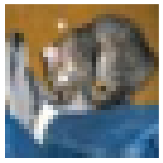
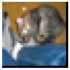
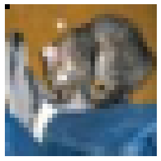
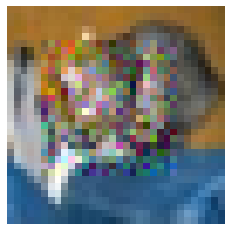
PM aims to quantify the level of privacy leakage regarding caused by , or in other words, it measures the dissimilarity between and in terms of human perception. However, common distance metrics like MSE fail to serve as an effective PM. These metrics are designed to only ensure high similarity between two inputs when their values are low. Unfortunately, the opposite conclusion does not always hold true. Consider Figure 3, where seemingly indistinguishable images to the human eye are deemed significantly different by MSE. Consequently, employing MSE may cause pseudo-privacy protections, highlighting the need for a better privacy metric.
3.3.2 Metric Design
Inspired by the above, we begin by summarizing the characteristic that an ideal PM should possess, named monotonicity principle: with the increasing value of , the privacy information involved in regarding should decrease monotonously. One intuitive idea for designing such a PM is to generate a reference sample for , which does not contain any private information associated with . This reference sample can then be exploited as a benchmark for evaluating privacy information contained in . The closer is to the reference sample, the less private information from will be embedded in . However, a key challenge arises: how to obtain a suitable reference sample?
At first glance, one might consider utilizing specific random noises222Random noises are considered as non-information samples [35]. as the reference sample. Though technically feasible, it produces a bottleneck for the performance of Refiner, because the search space is limited to the underlying route from to the specific reference sample. In other words, Refiner is unable to navigate other noise regions that may contain more informative samples. To address the problem, we define the distance of to the uniform distribution as our PM, i.e., the uniform distribution is our reference sample.
Let be distributed according to Dirac delta distribution that concentrates mass at 333In mathematical terms, Dirac delta distribution [41, 15] satisfies the integral property . function is zero everywhere except at the point , where it becomes infinite.. To measure the distance between and uniform noise distribution , we employ the JS divergence: . Unfortunately, directly evaluating JS divergence becomes computationally infeasible due to its high-dimensional nature. To this end, we leverage conjugate functions to reformulate JS divergence as follows (see Appendix A for details):
| (5) |
Practical Implementation. Equation 5 indicates the need to construct a new for each to estimate the JS divergence. To reduce costs, we search for a single for all images. The in this paper is a neural network dubbed the evaluation network, as DNNs are capable of approximating any function [17, 18]. Intuitively, the underlying goal of Equation 5 is to encourage to output 1 for random noises and 0 for natural samples. Essentially, the evaluation network indeed quantifies the proportion of noise within . This inspires us to create training data-label pairs for the network in an interpolate manner, i.e., , and these pairs are supplied into the network as supervised signals for training. Doing so enjoys that the monotonicity principle can be explicitly infused into the evaluation network.
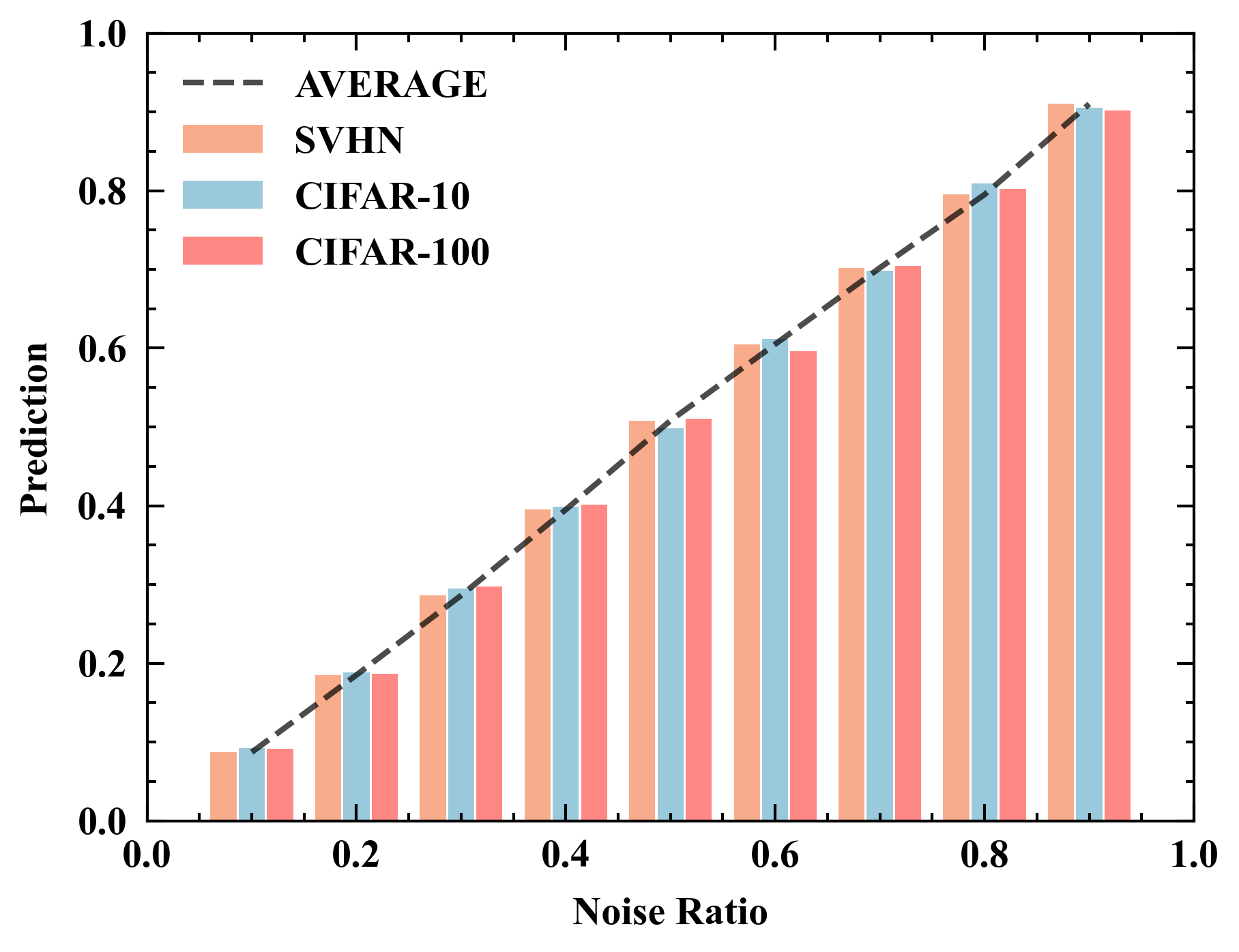
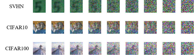
We use TinyImageNet dataset for training the evaluation network and more details can be found in Appendix D. Table 4 reports the predictions of the trained evaluation network for mixtures of random noises and natural images. An illustrative example is provided in Figure 5. Remarkably, the trained evaluation network performs well over different datasets like CIFAR-10, CIFAR-100, and SVHN, demonstrating its good generality. Moreover, it can be observed that when the noise ratio reaches approximately 0.6, human eyes are no longer able to identify privacy information. A byproduct of the evaluation network is its potential application as a privacy metric. In practical scenarios, clients can obtain the trained evaluation network from a trusted third party at no cost or train their own evaluation network using publicly available data. In this paper, all clients share this trained evaluation network by default.
3.4 Solving Optimization Task (Equation 2)


Upon defining the concrete forms of and , the remaining challenge is figuring out how to solve Equation 2. A straightforward solution is to harness gradient descent algorithm [6], which stands as one of the most commonly employed optimization algorithms. While gradient descent algorithm is capable of tackling optimization problems featuring solely convex terms like UM, it encounters obstacles when confronted with highly non-linear and non-convex neural networks like PM. Specifically, we initialize as , subsequently aiming to maximize PM(,), i.e., making noisy. As shown in Figure 6(b), the resulting deviate only slightly from (Figure 6(a)), yet the model confidently identifies it as a noisy sample. This phenomenon and are known as adversarial vulnerability and adversarial examples [13, 7].
To address the above problem, we propose noise-blended initialization, which by blending with random noises, i.e., . is a blend factor. A big value of enables to be initialized around the area flooding with noises. Subsequently, during the optimization process, the evaluation network will maintain as a noisy sample. Figure 6(c) exemplify the noise-blended initialization with . The resultant does not contain any semantic information regarding , showing the effectiveness of the noise-blended initialization.
4 Theoretical Analysis
This section conducts a theoretical analysis of Refiner from three fundamental dimensions, including performance maintenance, privacy protection, and time cost.
4.1 Performance Maintenance
Assumption 1
is -smooth: it holds that .
Assumption 2
is -strongly convex: there is .
Assumption 3
Let be uniformly random samples drawn from the local dataset of the -th client. The variance of stochastic gradients is bounded: Wherein, represents the gradients of model parameters computed across the complete local dataset .
Assumption 4
There exists a real number and the expected squared norm of stochastic gradients is uniformly bounded by : .
Theorem 1
Let Assumption 1, 2, 3, and 4 hold. Let be the optimal solution of Equation 2. Suppose the gradient distance associated with and is bounded: . Let represent the global optimal solution and () denote the local optimal solution for -th client. Choose . Let . There is:
where , and is initial parameters of the globally-shared model.
This subsection examines how Refiner contributes to the convergence of the global model. By establishing Assumption 1, 2, 3, and 4 and demonstrating Theorem 1 (proof available in the Appendix B), we shed light on the subsequent discussion. Theorem 1 provides an upper bound on the gap between the optimal solution and the model trained with Refiner after sufficient iterations. As the gradient distance between robust and client data decreases, this upper bound also decreases, implying better performance of the global model. This highlights the effectiveness behind minimizing the gradient distance between robust data and clients’ data in maintaining performance. The inclusion of the gradient distance term () in Equation 2 guarantees the boundedness of . In practice, we modify the gradients of robust data slightly. If the difference between the gradients of robust data and clients’ data exceeds , we search for the closest gradients within the -constraint and use them as the final uploaded gradients (see Appendix C for more details). Doing so enables us to evaluate the utility-privacy trade-off of Refiner by varying values of 444Adjusting the value of is also an alternative way, but we find that tuning is more convenient..
It is worth noting that FL commonly involves two scenarios: when the client data distributions are identical (IID) and non-identical (Non-IID). Our theoretical analysis does not require uniformity in the client data distributions. Thus, Theorem 1 is applicable to both scenarios. Moreover, these assumptions are consistent with [24] and aim to ensure a unique global extreme point, or that any local optimal point is also a global optimal point. For neural networks with multiple extreme points, Theorem 1 can be understood as guaranteeing convergence to at least one local extreme point.
4.2 Privacy Protection
There exist various types of GLAs, each with unique features. Analyzing the effectiveness of Refiner against each specific attack instance is cumbersome. Therefore, we begin by distilling GLAs into a generalized form by identifying patterns shared across attack instances. Then we analyze the effectiveness of Refiner against the generalized attack. In this way, our privacy analysis can be extended to encompass a wide spectrum of attack variations and potential evolving attacks.
GLAs exploit the mapping relationship between data and gradients to reconstruct high-fidelity data. Specifically, we represent the mapping relationship from data to gradients by . The objective of GLAs is to construct an inverse map from gradients to data that yields , thus enabling the recovery of clients’ data. Different GLAs can be derived by specifying the concrete form of 555In fact, and may not be one-to-one. But, after fixing random factors like random seeds, learning rate, etc., they have a unique solution and can be considered one-to-one. The term ”specified” here includes the meaning of fixing these factors.. Example 1, 2, and 3 are provided to demonstrate this.
Example 1
(Deep Leakage from Gradients (DLG) [54]). DLG’s inverse mapping is defined as the optimal solution to a gradient matching problem, which minimizes the -norm distance between the uploaded gradients and reconstructed data gradients: .
Example 2
Example 3
(Generative Gradient Leakage (GGA) [25]). GGA optimizes a latent input vector of a generative model to search data whose gradients align well with uploaded gradients. Moreover, GGA adds a KL divergence term to avoid too much deviation between the latent vector and the generator’s latent distribution: , where . is Gaussian distribution with a mean of 0 and a standard deviation of 1.
In practice, these attacks demonstrate superiority in recovering high-quality data. Therefore, their is quite similar to ground-truth one . Inspired by this, we make , where is a small positive number.
Refiner uploads the gradients associated with , which is denoted by . The server uses to recover data, i.e.. We now consider the distance of and :
| (6) |
Equation 6 establishes a lower bound of , which is determined by , , and . In practice, obtained by Equation 2 are often noisy and significantly differ from , i.e., (see Appendix F for the empirical validation). When is small, the lower bound can be simplified as follows:
| (7) |
Equation 7 suggests that a smaller results in higher privacy lower bound, i.e., stronger privacy protection capabilities. On the other hand, considering larger values of may be a little trivial. In detail, a larger leads to a significant discrepancy between the recovered data and clients’ data. Consequently, clients can directly upload ground-truth gradients since the attacker is unable to reconstruct high-fidelity data. In summary, the above analysis demonstrates the effectiveness and resilience of Refiner against GLAs, particularly those characterized by smaller values.
4.3 Time Complexity
| DP | GQ | Pruning | Soetria | Ours |
|---|---|---|---|---|
Before delving into the analysis of time complexity, it is essential to acknowledge that achieving excellence in all aspects of utility, privacy, and time is almost impossible. Because striking a better utility-privacy trade-off often necessitates additional time investment for searching. For instance, DP equally perturbs all gradient elements, without considering the inherent privacy information contained in each gradient element. In contrast, Soteria addresses this limitation by estimating the privacy information of each gradient element and selectively pruning those with the highest privacy information, resulting in an improved utility-privacy trade-off. However, this estimation process incurs additional time costs.
DP, GQ, and gradient pruning, none of which necessitate extra forward-backward propagations, are discussed together. DP generates noises for each gradient element, GQ quantizes each gradient element, and gradient pruning sorts and then removes part of gradient elements. By assuming the model of interest owns a total of parameters, the time complexity of both DP and GQ scales linearly with the number of parameters, . For gradient pruning, the dominant factor is the sorting time complexity, i.e., .
Soteria focuses on pruning gradients in the final fully connected layer. This entails a meticulous evaluation of the privacy information associated with each individual gradient element residing in the layer. Given that the total count of parameters contained within the layer to be denoted as , and the time complexity of once forward-backward propagation of the global model is . Soteria necessitates executing forward-backward propagation a specific number of times, corresponding to the number of neurons in the layer. Consequently, the overall time complexity of Soteria can be expressed as . The number of elements in a typical fully connected layer is usually .
The time complexity of Refiner primarily centers around solving Equation 2. Each iteration of Equation 2 requires twice forward-backward propagations of the global model, along with one forward-backward propagation of the evaluation network. Hence, the overall time complexity is the sum of these operations. Assuming the time complexity of running single forward-backward propagation for the evaluation network is and the total number of iterations for solving Equation 2 is , the time complexity of Refiner is . Table 3 summarizes the time complexities associated with these defenses. Section 6.2 conducts an empirical comparison of the time costs for these defenses.
5 Evaluation Setup
| Attack | iGLA | InvertingGrad | GradInvertion | GGA | ||||
|---|---|---|---|---|---|---|---|---|
| Loss Function | Euclidean | Cosine Similarity | Euclidean | Euclidean | ||||
| Regularization | None | TV |
|
|
||||
| Optimizer | L-BFGS | Adam | Adam | Adam | ||||
| Learning Rate | 1 | 0.01 | 0.01 | 0.01 | ||||
| Label Inference | ||||||||
| Attack Iteration | 300 | 4000 | 4000 | 4000 |
5.1 Attack
Four state-of-the-art attacks are considered to examine the performance of Refiner, including iGLA [53], GradInversion [48], InvertingGrad [12], GGA [25, 49]. These attacks cover the primary types of GLAs currently explored. The first three attacks address variants of Equation 1 by employing varying optimizers, loss functions, and so on. GGA, on the other hand, focuses on optimizing the latent vectors of a GAN to align the gradients. We implement these attacks at the start of training, as this stage is most vulnerable to GLAs [3]. For GGA, we use public codes 666https://raw.githubusercontent.com/pytorch/examples/master/dcgan/main.py to train a GAN. Table 4 provides an overview of the attack distinctions and the hyperparameters employed.
5.2 Competitor
We compare Refiner to the following defenses: DP [1], GQ [34, 49], gradient pruning [2, 54], and Soteria [44]777We use Soteria proposed in [44] to compare, which is an improved version compared with the original Soteria [39].. These defenses involve utility-privacy trade-offs that are regulated by hyperparameters such as noise magnitude for DP, discretization level for GQ, and pruning rate for pruning and Soteria. Stronger privacy protection can be achieved by increasing these hyperparameters, but this comes at the cost of performance degradation. We vary these hyperparameters to obtain the utility-privacy trade-off curves for each defense. Specifically, for DP, we employ two commonly used kinds of noises, namely Gaussian (DP-Gaussian) and Laplace (DP-Laplace), with magnitude ranging from to and of 1. As for GQ, we consider discretization levels, including 1, 2, 4, 8, 12, 16, 20, 24, and 28 bits. For pruning and Soteria, we set pruning ratio in . Besides, we alter of Refiner over (see Section 4.1). Unless specified otherwise, for Refiner, the default values of , , refinement iterations and are set to 0.5, 1, 10, and 0.95.
5.3 Evaluation Metric
We assess defenses from three fundamental dimensions: performance maintenance, privacy protection, and time cost.
Performance maintenance. We define the performance maintenance metric (PMM), which calculates the accuracy ratio achieved with defenses compared to the original accuracy without any defenses:
where and denote the accuracy of the model with and without defense888The original accuracies of LeNet are 84.12%, 54.01%, and 21.45% on SVHN, CIFAR10, and CIFAR100. The original accuracies of ResNet10 and ResNet18 are 83.25% and 84.95% on CIFAR10..
Privacy protection. Privacy protection measures the amount of privacy information recovered from the reconstructed images. Given the lack of a universally perfect privacy assessment metric, we employ a diverse range of metrics including PSNR [16], SSIM [45], LPIPS [51], and the evaluation network to achieve a more comprehensive assessment:
-
•
PSNR is the logarithmic average distance between the original and reconstructed images. A higher PSNR indicates high-quality reconstructed images.
-
•
SSIM captures human perception of image quality better by considering factors like brightness, contrast, and structure. SSIM ranges from 0 to 1, with values closer to 1 indicating greater similarity between two images.
-
•
LPIPS assesses the similarity of two images based on the comparison of features extracted by DNNs. A value close to 0 indicates a higher similarity between two images. LPIPS often better captures semantic and perceptual differences compared to PSNR and SSIM.
-
•
The evaluation network estimates the proportion of noise in the data, producing noise ratio between 0 and 1. As mentioned earlier, when the noise ratio exceeds 0.6, the human eye probably recognizes it as noisy data.
More details can be found in Appendix E.
Time cost. Time cost is also an important dimension for evaluating a defense. We record the time required for a single iteration of the model when employing defenses.
5.4 Model, Dataset, and Training Setting
We select two widely-used model architectures, LeNet [22] and ResNet [14], on three benchmark datasets SVHN [30], CIFAR10 [21], and CIFAR100 [21]. We include ResNet10 and ResNet18 to study the impact of different scales. Our focus is on a typical FL scenario involving 10 clients collaborating to train a global model, with the assistance of a server.
Our evaluation also examines the effect of data distribution on FL by considering both IID and non-IID settings [19]. In the IID setting, the training datasets are randomly and equally divided among the 10 clients, ensuring identical distribution for each client’s local dataset. In the Non-IID setting, we allocate the training datasets unevenly among the 10 clients in a label imbalance fashion [26, 19].
The training process takes place over 8000 iterations, during which each client computes gradients locally using a batch size of 128. These gradients are then uploaded to the server, which updates the global model using FedAvg with a learning rate of 0.01. We scale the data to the range of 0 to 1 without employing additional data augmentation techniques.
6 Empirical Evaluation

6.1 Privacy-Utility Trade-off
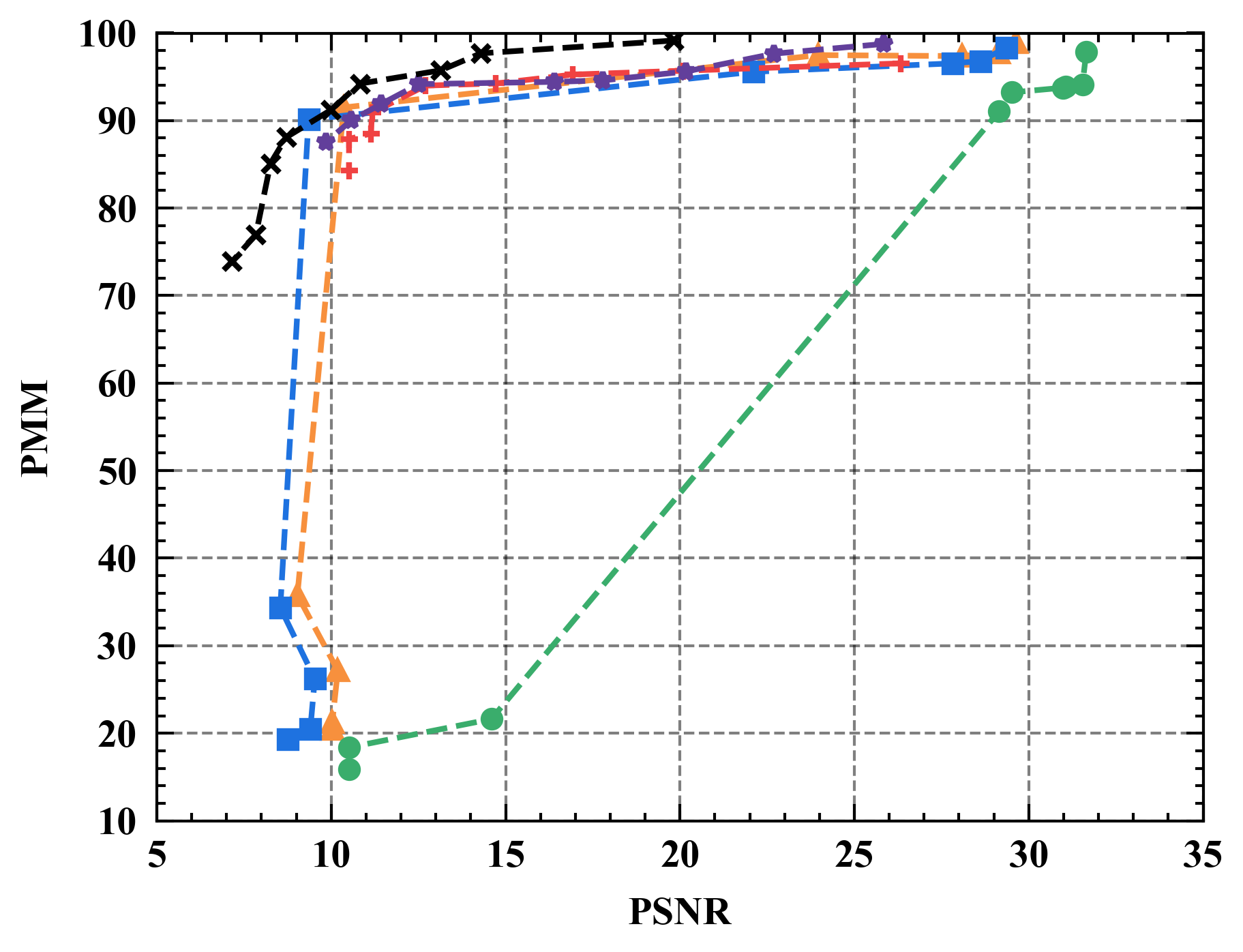
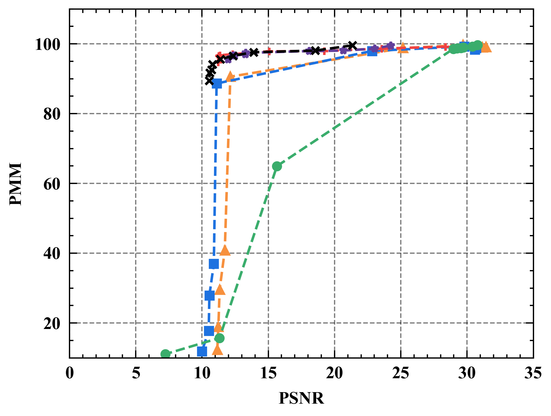
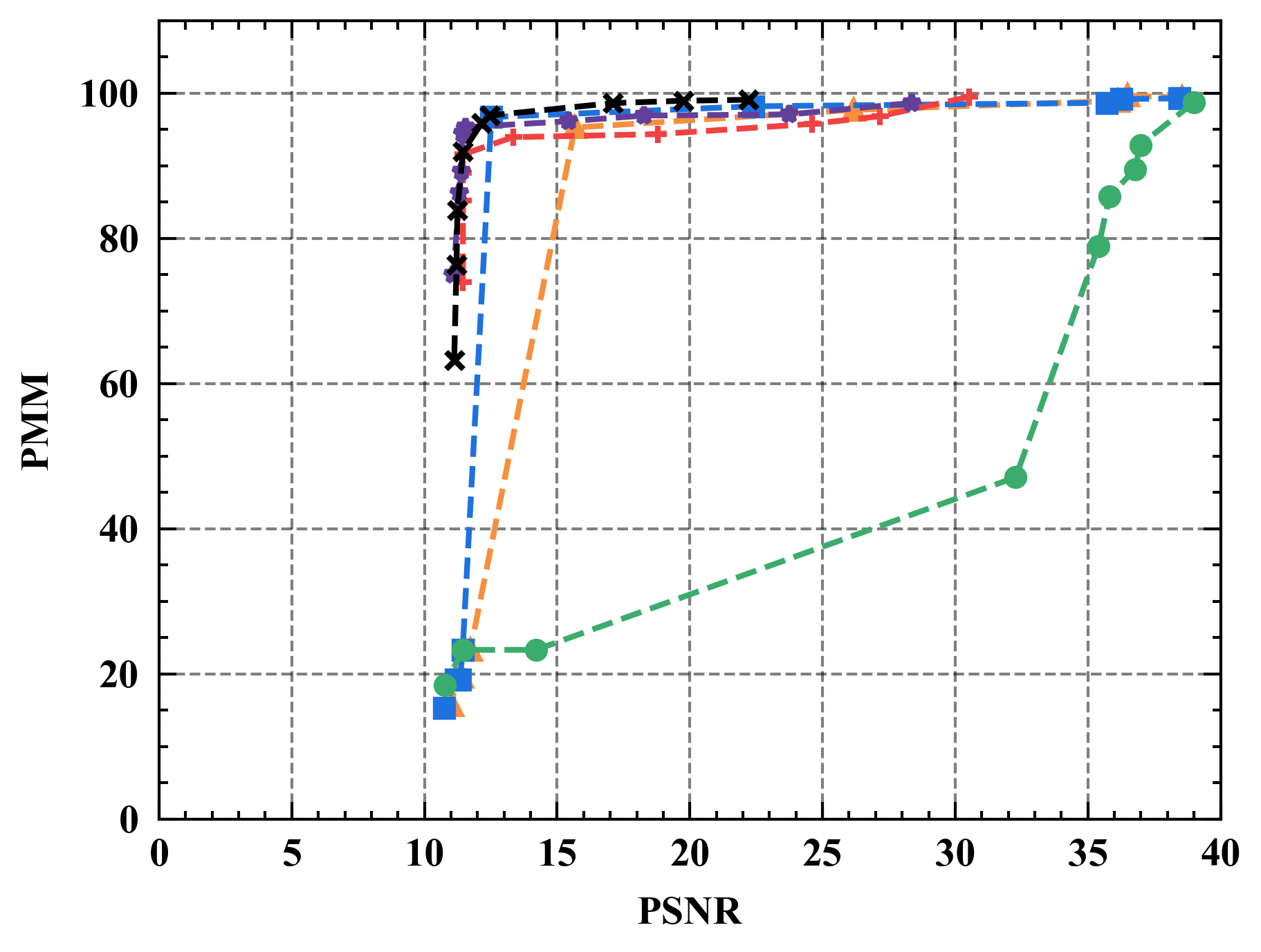
Numerical results. Figure 7 illustrates the trade-off curves between PMM (utility) and PSNR (privacy) for various defenses against four state-of-the-art attacks on CIFAR10. Overall, Refiner consistently outperforms baselines by achieving lower PSNR while maintaining comparable PMM. For instance, when employing InvertingGrad attack, Refiner obtains an improvement of approximately 3 in PSNR compared to state-of-the-art defense Soteria, while Refiner maintains slightly higher utility than Soteria.
Moreover, we observe that the impact of Refiner, Soteria, and Pruning on model performance is relatively mild compared to other defenses, except Refiner. Particularly, excessively aggressive defense strengths, such as employing a noise magnitude of DP greater than or equal to or employing a quantization precision less than or equal to 8 bits with GQ, can significantly deteriorate the model’s performance.
Semantic results. We see that the reconstruction quality of GGA, as measured by PSNR, is significantly inferior to the other three attacks. One possible explanation is that GGA focuses more on semantic rather than pixel-level reconstruction. To substantiate this conjecture, Figure 8 showcases the reconstruction images of GGA. Based on Figure 8, GGA indeed recovers the privacy information embedded in the original image (i.e., airplane), highlighting its attack effectiveness. Furthermore, compared to the PSNR metric, LPIPS places greater emphasis on the similarity of features extracted using DNNs, thereby underscoring the importance of semantic-level similarity over pixel-level similarity. Therefore, we deploy LPIPS metric and the evaluation network for further assessment of GGA’s effectiveness. From Figure 9(a), we observe that the attack performance of GGA is competitive with InvertingGrad against Soteria and Refiner. Remarkably, in Figure 9(b), the evaluation network consistently rates GGA’s attack effectiveness highly regardless of defense strength. This is intuitive since the generated images by GGA are noise-free, as displayed in Figure 8. In short, the above analysis stresses the necessity of employing diverse privacy metrics to assess defense performance.
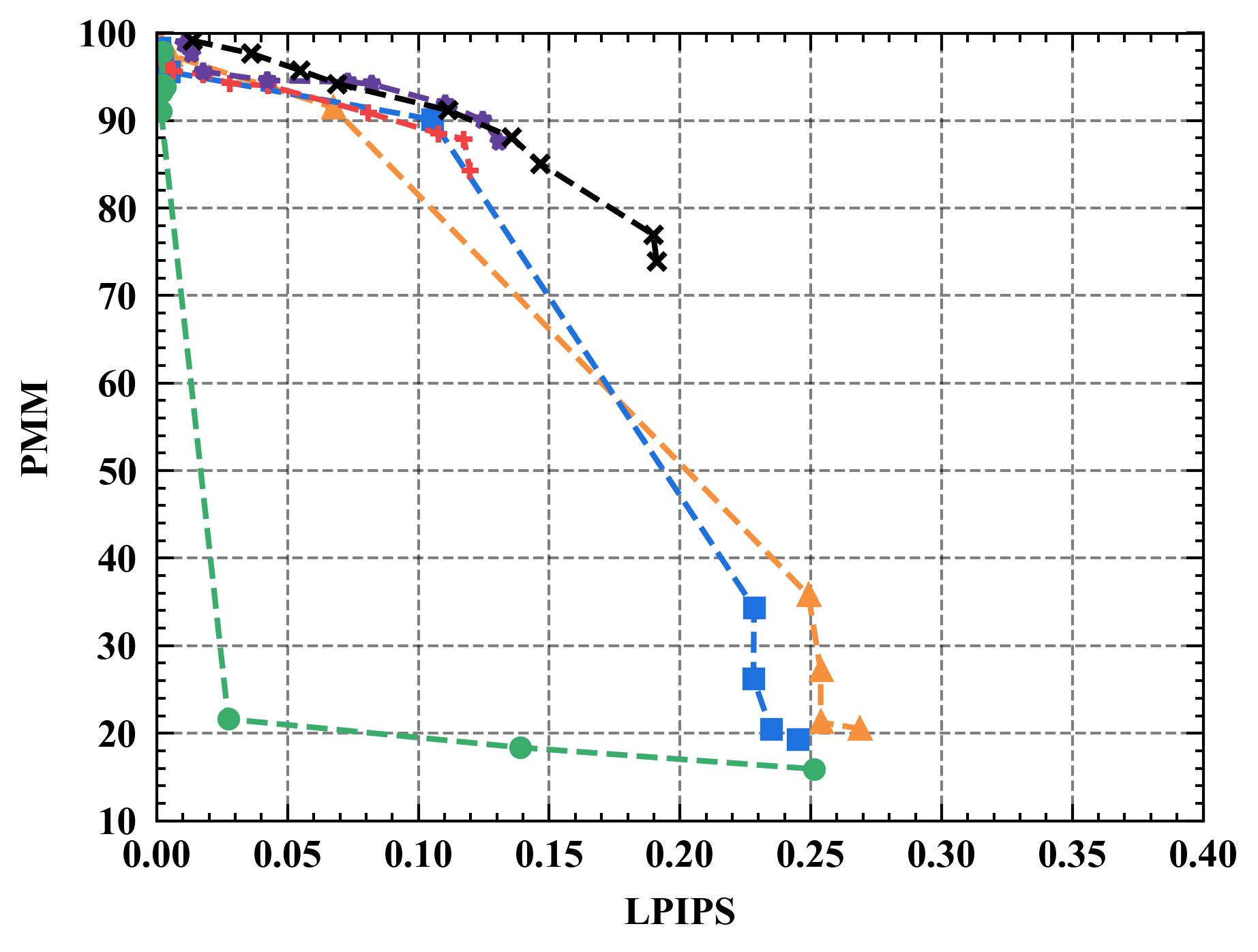
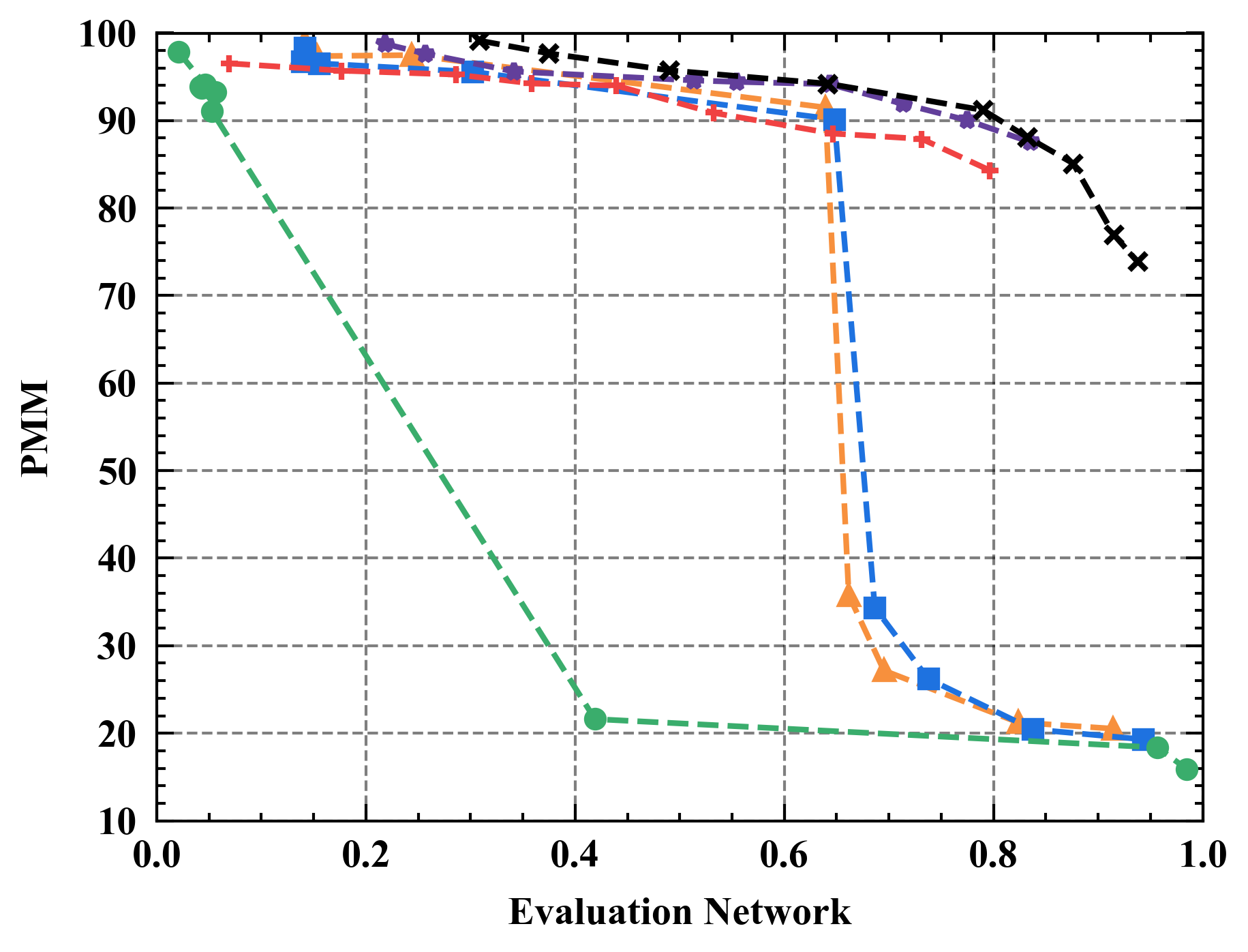
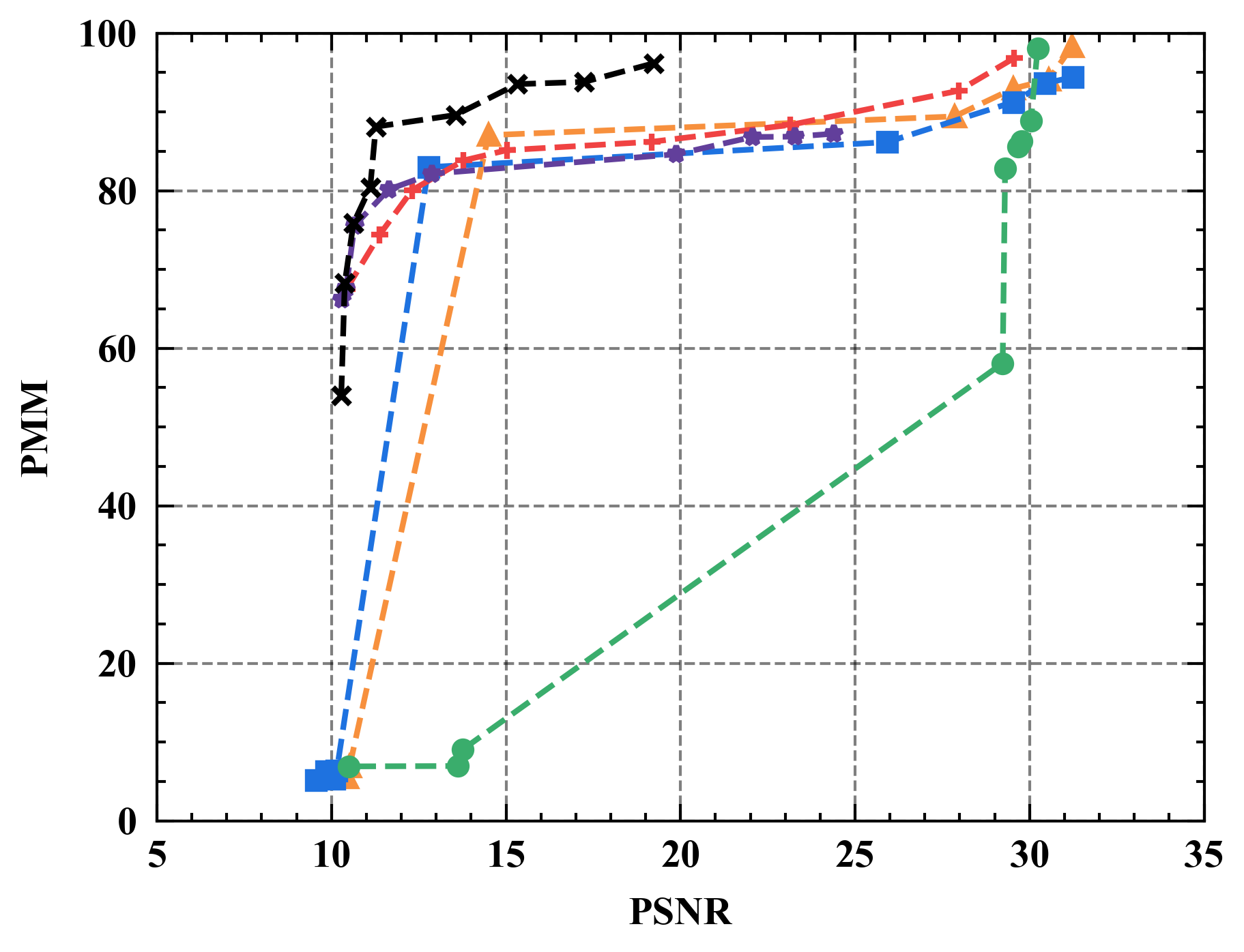
Evaluating defenses with varied assessment metrics. Figure 10 shows the performance of different defenses under various privacy metrics. As can be seen, Refiner consistently achieves a superior trade-off between privacy and utility when evaluated using different privacy metrics. For instance, Refiner enables the inclusion of approximately 30% noise information in constructed data with negligible impact on the model’s performance, whereas Soteria achieves only around 20% noise inclusion capability.
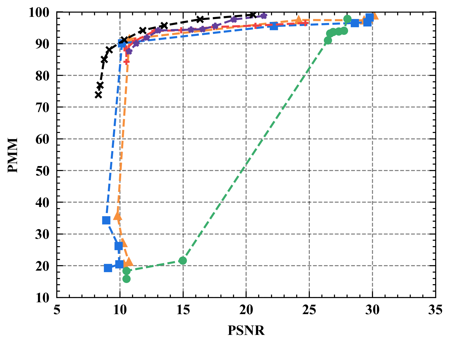
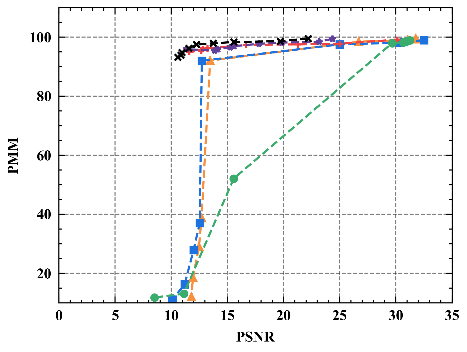
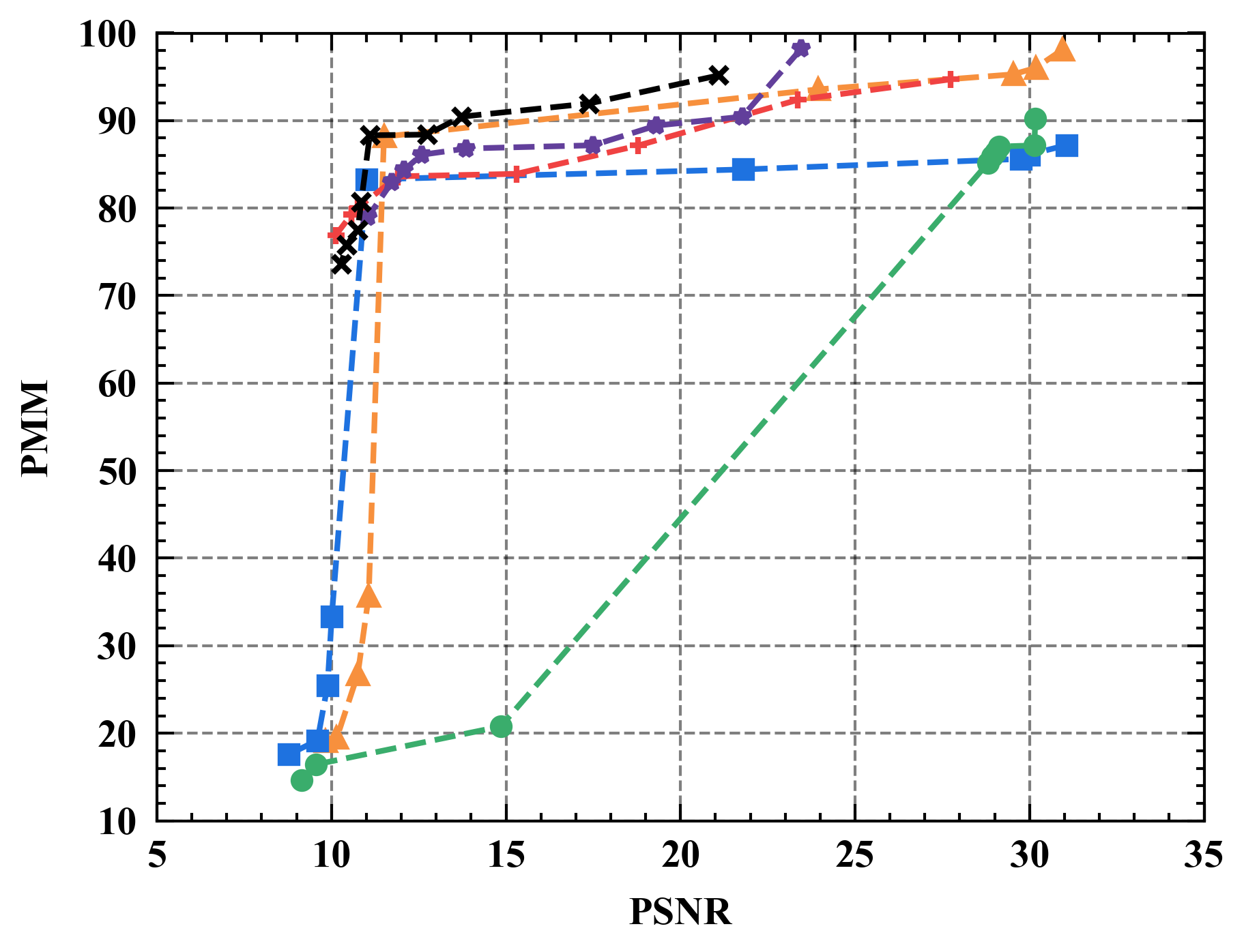
Safeguarding different model architectures. We here examine the performance of different defenses when applied to ResNet. The corresponding results are presented in Figure 11. Remarkably, Refiner exhibits a superior trade-off between utility and privacy, especially when applied to larger models (ResNet18) compared to baselines. We hypothesize that this can be attributed to the increased non-linearity capacity of larger models, rendering the assumptions of other defenses less valid and consequently leading to degraded effectiveness.
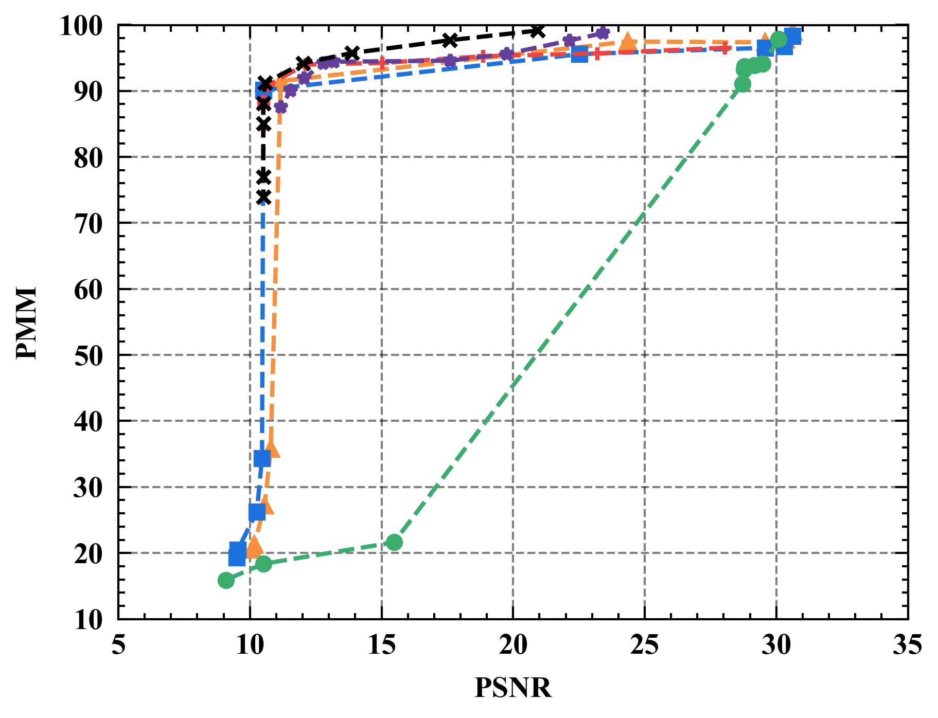
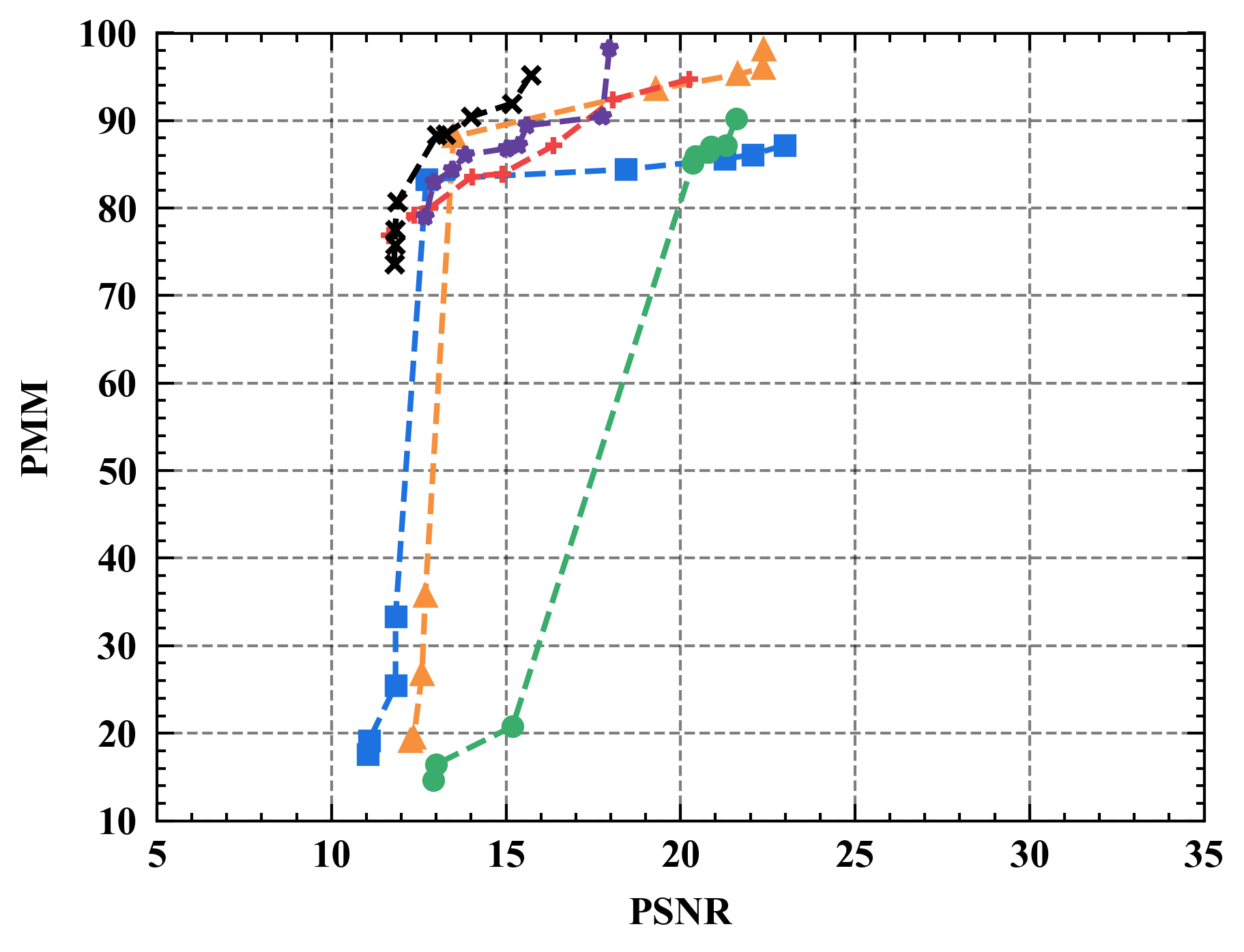
Safeguarding different datasets. We also evaluate the performance of Refiner on different datasets, SVHN and CIFAR100. The results not only confirm the consistent superior performance of Refiner, but also reveal two noteworthy observations. Firstly, we observe a better reconstruction quality for attacks carried out on SVHN, with the highest achieved PSNR approaching 40. This is probably because SVHN is a less sophisticated dataset, rendering the construction easier. Secondly, we observe the remarkable effectiveness of Refiner compared to baselines when applied to the CIFAR100 dataset, suggesting that Refiner exhibits greater resilience in handling more complex datasets.
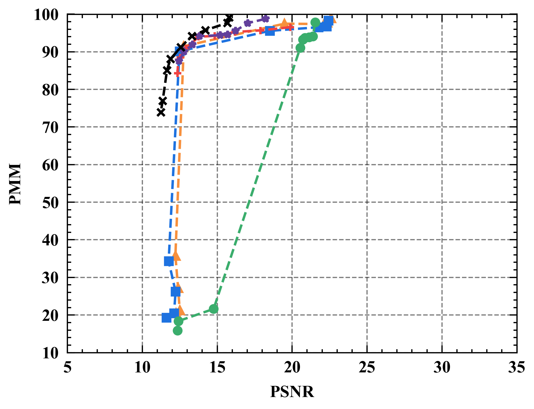
Defense with Non-IID setting. In the Non-IID setting, the datasets of clients are heterogeneous, posing greater challenges to maintaining performance. We evaluate the effectiveness of our approach in non-IID scenarios, as shown in Figure 13. Wherein, Refiner outperforms baselines. Moreover, while we observe little change in the quality of attacker-reconstructed images (measured by PSNR) under non-IID conditions, the difficulty of maintaining performance increases significantly compared to IID conditions.
| Dfense | LeNet | ResNet10 | ResNet18 | ResNet34 |
|---|---|---|---|---|
| Pruning | 0.0187 | 0.0495 | 0.0873 | 0.1370 |
| Gaussian | 0.0467 | 0.7317 | 1.8408 | 3.3020 |
| Laplace | 0.0469 | 0.7322 | 1.8414 | 3.3025 |
| GQ | 0.0179 | 0.0277 | 0.0514 | 0.1057 |
| Soteria | 0.4103 | 11.3148 | 21.7539 | 39.4410 |
| Our | 0.3340 | 1.7341 | 2.8539 | 4.7012 |
6.2 Empirical Time Complexity
The additional time cost they imposed by defenses is a crucial dimension of assessing their effectiveness. In this regard, Table 5 reports the runtime required for a single iteration of models when employing different defenses. For the small-scale model LeNet, Refiner and Soteria exhibit a time cost within the same order of magnitude. However, this time cost is one order of magnitude higher compared to Pruning, Gaussian, Laplace, and GQ. This is due to the fact that Refiner and Soteria require multiple forward-backward propagations to search for better utility-privacy trade-offs.
For larger models ResNet10 and ResNet18, The runtime required by Pruning and GQ increases in an approximate linear fashion. Refiner, Gaussian, and Laplace own comparable runtime overhead. Notably, Soteria incurs a significantly higher time cost of the 40s per iteration on ResNet34, which is 8.4x higher than the time required for Refiner. The heavy overhead of Soteria stems from the repeated execution of forward-backward propagation, which needs to be performed as many times as there are neurons in the fully connected layer. Consequently, as the number of fully connected neurons increases in larger models, the time cost of Soteria escalates significantly. In contrast, Refiner offers a scalable time cost for large models since the number of forward-backward propagations depends mainly on the user-specified number of iterations, granting flexibility based on factors such as clients’ privacy preferences and computing resources. Empirical results indicate that good performance can be achieved with only 10 iterations, far lower than the runtime cost associated with Soteria. In summary, Refiner achieves a better utility-privacy trade-off compared to DP, GQ, and gradient pruning, albeit at the expense of higher time cost. But, Refiner’s time cost is still lower than that of Soteria.
| PSNR | 13.89 | 13.62 | 13.44 | 13.20 | 13.08 | 12.70 | 12.04 |
| PMM | 91.93 | 91.12 | 91.06 | 90.69 | 90.00 | 89.30 | 88.90 |
| 5 | 10 | 15 | 20 | |
|---|---|---|---|---|
| PSNR | 13.05 | 13.20 | 13.37 | 13.45 |
| PMM | 85.61 | 90.69 | 91.19 | 92.17 |
| 0 | 0.1 | 0.3 | 0.5 | 0.7 | 0.9 | |
|---|---|---|---|---|---|---|
| PSNR | 21.24 | 16.52 | 14.99 | 13.20 | 12.53 | 10.52 |
| PMM | 98.52 | 95.45 | 92.61 | 90.69 | 90.08 | 89.34 |
| 0.91 | 0.93 | 0.95 | 0.97 | 1.00 | |
|---|---|---|---|---|---|
| PSNR | 12.93 | 13.05 | 13.10 | 13.15 | 15.44 |
| PMM | 90.98 | 90.82 | 90.69 | 90.46 | 89.28 |
6.3 Sub-components Analysis
In this section, we investigate the impact of four sub-components of Refiner on its performance. We fix .
Impact of balance factor . Table 6 reports the performance of Refiner as varies against InvertingGrad. Overall, the higher is, the lower PMM is, and the higher MSE is. Moreover, the performance of Refiner is more robust to tuning compared with , i.e., there is not a huge performance shift w.r.t. different . Thus, we believe setting by default is a good option in practice.
Impact of refinement iterations . Refinement iterations can influence the quality of resultant robust data and Table 7 reports the performance of Refiner over different refinement iterations against InvertingGrad. An observation is that, the performance of Refiner intensively increases by raising refinement iterations from 1 to 100, but further enhancing refinement iterations from 100 to 200 only produces a slight improvement, suggesting that refinement iterations of 100 are sufficient for optimization convergence in practice.
Impact of . Table 8 reports the performance of Refiner when configured with varying refinement iteration settings against InvertingGrad. It is observed that increasing the refinement iterations from 5 to 10 leads to a significant improvement in the performance of Refiner, enabling the acquisition of more PMM with similar PSNR (similar privacy protection ability). Intuitively, this is because during the early iterations, Refiner can maintain robust data to be noisy while effectively aligning gradients associated with clients’ and robust data. Further increasing the refinement iterations to 15 or 20 only yields marginal enhancements, suggesting that a refinement iteration value of approximately 10 would be a preferable choice for practical applications if considering the time cost.
Impact of . When considering the promotion of the alignment between client data and robust data gradients, plays a significant role. It directs more attention towards aligning the gradients of early layers, serving a dual purpose. Firstly, it aids in maintaining the performance of the model since the early layers contribute more significantly to its performance. Secondly, according to [39], the issue of privacy leakage is more closely associated with the gradients of later layers. The experimental results are summarized in Table 9. By including in Refiner, i.e., a transition from 1 to 0.97, we see only a marginal 1% decrease in PMM, yet achieve a substantial 2-point reduction in PSNR. Further increasing the value of does not yield significant changes in PSNR and PMM, suggesting that the observed improvements reach a plateau.
7 Discussion and Future Work
Why does Refiner work? We are interested in understanding why Refiner is more effective than perturbation-based methods. We find that perturbation-based methods exhibit optimality under specific assumptions. However, these assumptions rarely hold true for DNNs, thereby posing a challenge to achieving the desired performance using these methods.
To elaborate, perturbing each gradient element equally, as commonly practiced in DP and GQ, assumes that every gradient element carries an equal amount of privacy information and contributes equally to the model performance. Under this assumption, the optimal utility-privacy trade-off can be reached through uniformly perturbing fashions. By regarding all gradient elements as possessing identical privacy information, the optimal solution, derived from Taylor expansion, suggests preserving the gradient elements with the highest magnitudes, i.e.gradient pruning. Soteria takes into account the linearity assumption of DNNs, allowing for an estimation of the privacy information contained in each gradient element as well as assuming the same utility across all gradient elements. In this way, Soteria can theoretically achieve optimality by selectively removing the gradient elements with the highest privacy information.
When employing Refiner, clients upload the gradients associated with robust data that are generated by optimizing two metrics for privacy protection and performance maintenance. The uploaded gradients in Refiner only involve privacy from robust data. By reducing semantic similarity between the robust data and clients’ data, the uploaded gradients contain less privacy information associated with clients’ data. Importantly, such privacy estimation fashion avoids potential estimation errors that may arise from questionable assumptions made by perturbation-based methods. Regarding utility, Refiner prioritizes important parameters and narrows the gap between the gradients of these parameters with respect to robust and clients’ data. Section 3.3 validates that preserving the gradient of important parameters is a better solution than retaining gradients with the largest magnitude, i.e., gradient pruning. Taken together, we grasp why Refiner enjoys so impressive performance compared to perturbation-based methods.
Limitation and future work. The superior performance of Refiner is accompanied by a higher time cost compared to DP, GQ, and gradient pruning, but still lower than Soteria. The non-negligible extra time costs constitute the major drawback of Refiner, probably making some difficulty in its implementation over resource-constrained clients. However, it should be acknowledged that higher performance commonly entails increased computational resources as a trade-off, specifically in deep learning field. In summary, we believe that Refiner introduces a novel idea along with a pair of concrete privacy and utility metrics for mitigating GLAs. In future endeavors, our focus will be on reducing the time cost associated with Refiner, so as to extend it to be more suitable to resource-constrained scenarios.
References
- Abadi et al. [2016] Martin Abadi, Andy Chu, Ian Goodfellow, H Brendan McMahan, Ilya Mironov, Kunal Talwar, and Li Zhang. Deep learning with differential privacy. In Proceedings of the 2016 ACM SIGSAC conference on computer and communications security, pages 308–318, 2016.
- Aji and Heafield [2017] Alham Fikri Aji and Kenneth Heafield. Sparse communication for distributed gradient descent. ArXiv, abs/1704.05021, 2017. URL https://api.semanticscholar.org/CorpusID:2140766.
- Balunović et al. [2022] Mislav Balunović, Dimitar I Dimitrov, Robin Staab, and Martin Vechev. Bayesian framework for gradient leakage. In International Conference on Learning Representations, 2022.
- Bernstein et al. [2018] Jeremy Bernstein, Yu-Xiang Wang, Kamyar Azizzadenesheli, and Anima Anandkumar. signsgd: compressed optimisation for non-convex problems. In International Conference on Machine Learning, 2018. URL https://api.semanticscholar.org/CorpusID:7763588.
- Bonawitz et al. [2017] Keith Bonawitz, Vladimir Ivanov, Ben Kreuter, Antonio Marcedone, H. B. McMahan, Sarvar Patel, Daniel Ramage, Aaron Segal, and Karn Seth. Practical secure aggregation for privacy-preserving machine learning. Proceedings of the 2017 ACM SIGSAC Conference on Computer and Communications Security, 2017. URL https://api.semanticscholar.org/CorpusID:3833774.
- Boyd and Vandenberghe [2005] Stephen P. Boyd and Lieven Vandenberghe. Convex optimization. Journal of the American Statistical Association, 100:1097 – 1097, 2005. URL https://api.semanticscholar.org/CorpusID:37925315.
- Carlini and Wagner [2016] Nicholas Carlini and David A. Wagner. Towards evaluating the robustness of neural networks. 2017 IEEE Symposium on Security and Privacy (SP), pages 39–57, 2016. URL https://api.semanticscholar.org/CorpusID:2893830.
- Dowlin et al. [2016] Nathan Dowlin, Ran Gilad-Bachrach, Kim Laine, Kristin E. Lauter, Michael Naehrig, and John Robert Wernsing. Cryptonets: applying neural networks to encrypted data with high throughput and accuracy. In International Conference on Machine Learning, 2016.
- Fan et al. [2022] Mingyuan Fan, Yang Liu, Cen Chen, Shengxing Yu, W. Guo, Li Wang, and Ximeng Liu. Toward evaluating the reliability of deep-neural-network-based iot devices. IEEE Internet of Things Journal, 9:17002–17013, 2022. URL https://api.semanticscholar.org/CorpusID:245560775.
- Fereidooni et al. [2021] Hossein Fereidooni, Samuel Marchal, Markus Miettinen, Azalia Mirhoseini, Helen Möllering, Thien Duc Nguyen, Phillip Rieger, Ahmad-Reza Sadeghi, T. Schneider, Hossein Yalame, and Shaza Zeitouni. Safelearn: Secure aggregation for private federated learning. 2021 IEEE Security and Privacy Workshops (SPW), pages 56–62, 2021. URL https://api.semanticscholar.org/CorpusID:233176356.
- Geert et al. [2017] Geert, Litjens, Thijs, Kooi, Babak, Ehteshami, Bejnordi, Arnaud, Arindra, and Adiyoso. A survey on deep learning in medical image analysis. Medical Image Analysis, 2017.
- Geiping et al. [2020] Jonas Geiping, Hartmut Bauermeister, Hannah Dröge, and Michael Moeller. Inverting gradients-how easy is it to break privacy in federated learning? Advances in Neural Information Processing Systems, 33:16937–16947, 2020.
- Goodfellow et al. [2014] Ian J. Goodfellow, Jonathon Shlens, and Christian Szegedy. Explaining and harnessing adversarial examples. In International Conference on Learning Representations, 2014.
- He et al. [2015] Kaiming He, X. Zhang, Shaoqing Ren, and Jian Sun. Deep residual learning for image recognition. 2016 IEEE Conference on Computer Vision and Pattern Recognition (CVPR), pages 770–778, 2015. URL https://api.semanticscholar.org/CorpusID:206594692.
- Hoff [2009] Peter D. Hoff. A first course in bayesian statistical methods. 2009. URL https://api.semanticscholar.org/CorpusID:60995805.
- Horé and Ziou [2010] Alain Horé and Djemel Ziou. Image quality metrics: Psnr vs. ssim. 2010 20th International Conference on Pattern Recognition, pages 2366–2369, 2010. URL https://api.semanticscholar.org/CorpusID:9506273.
- Hornik et al. [1989] Kurt Hornik, Maxwell B. Stinchcombe, and Halbert L. White. Multilayer feedforward networks are universal approximators. Neural Networks, 2:359–366, 1989. URL https://api.semanticscholar.org/CorpusID:2757547.
- Hornik et al. [1990] Kurt Hornik, Maxwell B. Stinchcombe, and Halbert L. White. Universal approximation of an unknown mapping and its derivatives using multilayer feedforward networks. Neural Networks, 3:551–560, 1990. URL https://api.semanticscholar.org/CorpusID:13533363.
- Hsu et al. [2019] Tzu-Ming Harry Hsu, Qi, and Matthew Brown. Measuring the effects of non-identical data distribution for federated visual classification. ArXiv, abs/1909.06335, 2019. URL https://api.semanticscholar.org/CorpusID:202572978.
- Jeon et al. [2021] Jinwoo Jeon, Kangwook Lee, Sewoong Oh, Jungseul Ok, et al. Gradient inversion with generative image prior. Advances in Neural Information Processing Systems, 34:29898–29908, 2021.
- Krizhevsky [2009] Alex Krizhevsky. Learning multiple layers of features from tiny images. 2009. URL https://api.semanticscholar.org/CorpusID:18268744.
- LeCun et al. [1998] Yann LeCun, Léon Bottou, Yoshua Bengio, and Patrick Haffner. Gradient-based learning applied to document recognition. Proc. IEEE, 86:2278–2324, 1998. URL https://api.semanticscholar.org/CorpusID:14542261.
- Li et al. [2020a] Tian Li, Anit Kumar Sahu, Ameet Talwalkar, and Virginia Smith. Federated learning: Challenges, methods, and future directions. IEEE Signal Processing Magazine, 37(3):50–60, 2020a.
- Li et al. [2020b] Xiang Li, Kaixuan Huang, Wenhao Yang, Shusen Wang, and Zhihua Zhang. On the convergence of fedavg on non-iid data. 2020b.
- Li et al. [2022] Zhuohang Li, Jiaxin Zhang, Luyang Liu, and Jian Liu. Auditing privacy defenses in federated learning via generative gradient leakage. In Proceedings of the IEEE/CVF Conference on Computer Vision and Pattern Recognition, pages 10132–10142, 2022.
- MacKay [2004] David John Cameron MacKay. Information theory, inference, and learning algorithms. IEEE Transactions on Information Theory, 50:2544–2545, 2004. URL https://api.semanticscholar.org/CorpusID:5436619.
- McMahan et al. [2016] H. B. McMahan, Eider Moore, Daniel Ramage, Seth Hampson, and Blaise Agüera y Arcas. Communication-efficient learning of deep networks from decentralized data. In International Conference on Artificial Intelligence and Statistics, 2016. URL https://api.semanticscholar.org/CorpusID:14955348.
- Mohassel and Zhang [2017] Payman Mohassel and Yupeng Zhang. Secureml: A system for scalable privacy-preserving machine learning. 2017 IEEE Symposium on Security and Privacy (SP), pages 19–38, 2017. URL https://api.semanticscholar.org/CorpusID:11605311.
- Moshayedi et al. [2022] Ata Jahangir Moshayedi, Atanu Shuvam Roy, Amin Kolahdooz, and Yang Shuxin. Deep learning application pros and cons over algorithm. EAI Endorsed Transactions on AI and Robotics, 2022. URL https://api.semanticscholar.org/CorpusID:247311133.
- Netzer et al. [2011] Yuval Netzer, Tao Wang, Adam Coates, A. Bissacco, Bo Wu, and A. Ng. Reading digits in natural images with unsupervised feature learning. 2011. URL https://api.semanticscholar.org/CorpusID:16852518.
- Nweke et al. [2019] Henry Friday Nweke, Ying Wah Teh, Ghulam Mujtaba, and Mohammed Ali Al-Garadi. Data fusion and multiple classifier systems for human activity detection and health monitoring: Review and open research directions. Information Fusion, 46:147–170, 2019.
- OpenAI [2023] OpenAI. Gpt-4 technical report. ArXiv, abs/2303.08774, 2023. URL https://api.semanticscholar.org/CorpusID:257532815.
- Pouyanfar et al. [2018] Samira Pouyanfar, Saad Sadiq, Yilin Yan, Haiman Tian, Yudong Tao, Maria Presa Reyes, Mei-Ling Shyu, Shu-Ching Chen, and Sundaraja S Iyengar. A survey on deep learning: Algorithms, techniques, and applications. ACM Computing Surveys (CSUR), 51(5):1–36, 2018.
- Reisizadeh et al. [2019] Amirhossein Reisizadeh, Aryan Mokhtari, Hamed Hassani, Ali Jadbabaie, and Ramtin Pedarsani. Fedpaq: A communication-efficient federated learning method with periodic averaging and quantization. In International Conference on Artificial Intelligence and Statistics, 2019. URL https://api.semanticscholar.org/CorpusID:203593931.
- Reza [1994] Fazlollah M Reza. An introduction to information theory. Courier Corporation, 1994.
- Russakovsky et al. [2014] Olga Russakovsky, Jia Deng, Hao Su, Jonathan Krause, Sanjeev Satheesh, Sean Ma, Zhiheng Huang, Andrej Karpathy, Aditya Khosla, Michael S. Bernstein, Alexander C. Berg, and Li Fei-Fei. Imagenet large scale visual recognition challenge. International Journal of Computer Vision, 115:211 – 252, 2014. URL https://api.semanticscholar.org/CorpusID:2930547.
- Sahu et al. [2018] Anit Kumar Sahu, Tian Li, Maziar Sanjabi, Manzil Zaheer, Ameet Talwalkar, and Virginia Smith. Federated optimization in heterogeneous networks. arXiv: Learning, 2018. URL https://api.semanticscholar.org/CorpusID:59316566.
- Schuhmann et al. [2022] Christoph Schuhmann, Romain Beaumont, Richard Vencu, Cade Gordon, Ross Wightman, Mehdi Cherti, Theo Coombes, Aarush Katta, Clayton Mullis, Mitchell Wortsman, Patrick Schramowski, Srivatsa Kundurthy, Katherine Crowson, Ludwig Schmidt, Robert Kaczmarczyk, and Jenia Jitsev. Laion-5b: An open large-scale dataset for training next generation image-text models. ArXiv, abs/2210.08402, 2022. URL https://api.semanticscholar.org/CorpusID:252917726.
- Sun et al. [2021] Jingwei Sun, Ang Li, Binghui Wang, Huanrui Yang, Hai Li, and Yiran Chen. Soteria: Provable defense against privacy leakage in federated learning from representation perspective. In Proceedings of the IEEE/CVF Conference on Computer Vision and Pattern Recognition, pages 9311–9319, 2021.
- Suárez et al. [2021] Juan Luis Suárez, Salvador García, and Francisco Herrera. A tutorial on distance metric learning: Mathematical foundations, algorithms, experimental analysis, prospects and challenges. Neurocomputing, 425:300–322, 2021. ISSN 0925-2312. doi: https://doi.org/10.1016/j.neucom.2020.08.017. URL https://www.sciencedirect.com/science/article/pii/S0925231220312777.
- Theodoridis [2015] Sergios Theodoridis. Machine learning: a Bayesian and optimization perspective. Academic press, 2015.
- Vepakomma et al. [2018] Praneeth Vepakomma, Otkrist Gupta, Tristan Swedish, and Ramesh Raskar. Split learning for health: Distributed deep learning without sharing raw patient data. ArXiv, abs/1812.00564, 2018. URL https://api.semanticscholar.org/CorpusID:54439509.
- Wainakh et al. [2021] Aidmar Wainakh, Till Müßig, Tim Grube, and Max Mühlhäuser. Label leakage from gradients in distributed machine learning. 2021 IEEE 18th Annual Consumer Communications & Networking Conference (CCNC), pages 1–4, 2021. URL https://api.semanticscholar.org/CorpusID:232266184.
- Wang et al. [2022] Junxiao Wang, Song Guo, Xin Xie, and Heng Qi. Protect privacy from gradient leakage attack in federated learning. In IEEE INFOCOM 2022-IEEE Conference on Computer Communications, pages 580–589. IEEE, 2022.
- Wang et al. [2004] Zhou Wang, Alan Conrad Bovik, Hamid R. Sheikh, and Eero P. Simoncelli. Image quality assessment: from error visibility to structural similarity. IEEE Transactions on Image Processing, 13:600–612, 2004. URL https://api.semanticscholar.org/CorpusID:207761262.
- Wei et al. [2020] Wenqi Wei, Ling Liu, Margaret Loper, Ka-Ho Chow, Mehmet Emre Gursoy, Stacey Truex, and Yanzhao Wu. A framework for evaluating client privacy leakages in federated learning. In European Symposium on Research in Computer Security, pages 545–566. Springer, 2020.
- Wei et al. [2021] Wenqi Wei, Ling Liu, Yanzhao Wut, Gong Su, and Arun Iyengar. Gradient-leakage resilient federated learning. In 2021 IEEE 41st International Conference on Distributed Computing Systems (ICDCS), pages 797–807. IEEE, 2021.
- Yin et al. [2021] Hongxu Yin, Arun Mallya, Arash Vahdat, Jose M Alvarez, Jan Kautz, and Pavlo Molchanov. See through gradients: Image batch recovery via gradinversion. In Proceedings of the IEEE/CVF Conference on Computer Vision and Pattern Recognition, pages 16337–16346, 2021.
- Yue et al. [2023] K. Yue, Richeng Jin, Chau-Wai Wong, Dror Baron, and Huaiyu Dai. Gradient obfuscation gives a false sense of security in federated learning. 32nd USENIX Security Symposium (USENIX Security 23), 2023.
- Zhang et al. [2020] Chengliang Zhang, Suyi Li, Junzhe Xia, Wei Wang, Feng Yan, and Yang Liu. Batchcrypt: Efficient homomorphic encryption for cross-silo federated learning. In USENIX Annual Technical Conference, 2020.
- Zhang et al. [2018] Richard Zhang, Phillip Isola, Alexei A. Efros, Eli Shechtman, and Oliver Wang. The unreasonable effectiveness of deep features as a perceptual metric. 2018 IEEE/CVF Conference on Computer Vision and Pattern Recognition, pages 586–595, 2018. URL https://api.semanticscholar.org/CorpusID:4766599.
- Zhang et al. [2022] Rui Zhang, Song Guo, Junxiao Wang, Xin Xie, and Dacheng Tao. A survey on gradient inversion: Attacks, defenses and future directions. ArXiv, abs/2206.07284, 2022. URL https://api.semanticscholar.org/CorpusID:249674534.
- Zhao et al. [2020] Bo Zhao, Konda Reddy Mopuri, and Hakan Bilen. idlg: Improved deep leakage from gradients. arXiv preprint arXiv:2001.02610, 2020.
- Zhu et al. [2019] Ligeng Zhu, Zhijian Liu, and Song Han. Deep leakage from gradients. Advances in Neural Information Processing Systems, 32, 2019.
Appendix A Proof of Privacy Metric
We here prove the following equation:
| (8) |
A convex function can be represented using its conjugate form as follows:
| (9) |
where belongs to the range of . Equation 9 indicates that the value of at a certain point can be evaluated by maximizing . When given an , there exists a fixed corresponding value for , which we denote as . Consequently, Equation 9 can be rewritten as follows:
| (10) |
where the range of belongs to the range of .
Now let’s return to the JS divergence of and . Upon reorganization, we obtain the following expression of JS divergence:
| (11) |
Let’s consider letting and define . It is easy to verify that is a convex function over its domain ranging from to . Figure 14 shows the shape of .
Now we represent JS divergence using its conjugate form as follows:
| (12) |
According to Equation 10, the corresponding form of to is . Substituting the specific form of into Equation 12, we obtain:
| (13) |
Setting and substituting it into Equation 13, we obtain:
| (14) |
Equation 5 and Equation 14 differ only in the absence of and , which do not affect the final results. Moreover, the definition of conjugate function requires to be limited to the range of . Since the range of is smaller than , we can derive that the range of is constrained to the interval of 0 to 1.
Appendix B Proof of Theorem 1
Based on Assumption 4, we obtain:
| (16) |
Appendix C Projection Algorithm
Appendix D More Detailed Settings
The architecture and training settings of the evaluation network. The evaluation network used in this paper consists of four layers: three convolutional layers with Relu activation function followed by a fully connected layer with a sigmoid function. The size of the convolutional kernels is , with a stride of 2 and padding of 1. The number of convolutional kernels in the three convolutional layers is 128, 256, and 512, respectively. The last convolutional layer’s output is flattened to match the required input size of the fully connected layer. The output dimension of the fully connected layer is 1, meaning that it predicts the proportion of noises in given inputs. We optimize the evaluation network using the Adam optimizer with a learning rate of , batch size of 128, trained for 20 epochs. The evaluation network is trained by randomly mixing random noises into each batch eleven times using (the value of also is supervised signals) before iterating on the next batch.
Non-IID setting. Here we elaborate on how to generate non-IID datasets of clients. We assign a local distribution for each client, representing the distribution of data categories in local datasets. To achieve this, we employ a symmetric Dirichlet distribution with a concentration parameter of 1. By independently sampling from this distribution for each client, we determine the number of samples associated with specific labels that the client possesses. Finally, we randomly select a specified number of samples from training dataset to form the non-IID local datasets. These datasets are used in Section 6 to evaluate the effectiveness of different defenses.
Appendix E Concrete Formula of Evaluation Metrics
We here elaborate on the metrics used in this paper, including PSNR, SSIM, and LPIPS. The evaluation network has been detailed in Section 3.3. Consider the images of interest, denoted as . represent the dimensions of channels, heights, and weights for the images.
PSNR (Peak Signal-to-Noise Ratio). PSNR serves as a useful benchmark to evaluate the quality of reconstructed images compared to the original. It quantifies the level of noise or distortion present in reconstructed images by comparing the mean square error (MSE) between the original and reconstructed images. The formula for PSNR can be expressed as follows:
| (17) |
MSE is the mean square error between the original and reconstructed images and is the maximum possible pixel value (e.g., 255 for an 8-bit image). In our evaluation, images are scaled within the range of 0 to 1. Thus, equals 1.
SSIM (Structural Similarity Index). The SSIM metric gauges the degree of structural similarity between two images, by accounting for differences in their luminance, contrast, and structure. The index ranges from 0 to 1, with a score of 1 indicating complete similarity. The formula for SSIM is:
where , are the mean values of and , , are the variances of and , is their covariance, and and are small constants added for promoting numerical stability. In this paper, we call the off-the-shelf SSIM function provided by the skimage library 999https://github.com/scikit-image/scikit-image to directly compute the SSIM score for a pair of images.
LPIPS (Learned Perceptual Image Patch Similarity). LPIPS assesses the perceptual similarity of two images by leveraging convolutional neural networks. It calculates the dissimilarity between feature representations extracted from convolutional neural networks. Let us denote the extracted features of images as . In this case, the LPIPS is given by:
Here, represents the predefined coefficients that weight the different channels. denotes the value of -th channel’s element at -th row and -th column in the feature map . For practical implementation, we employ the LPIPS function provided by the open-source library lpips 101010https://github.com/richzhang/PerceptualSimilarity, which is built upon the AlexNet backbone.
Appendix F Supplementary Evidence Supporting Section 4.2
| Attack | iGLA | GradInvertion | InvertingGrad | GGA |
|---|---|---|---|---|
| 0.00018 | 0.00053 | 0.00046 | 0.00594 |
We here empirically demonstrate that , where represents the distance between and the reconstructed data using gradients associated with . We randomly extract 1000 from the training set of CIFAR10 as . We utilize LeNet and follow the same configuration as in Section 5. Table 10 reports the MSE distance averaged over 1000 samples using four different attack methods. We further construct robust data for these 1000 samples. The MSE distance, averaged over these 1000 samples, between and their robust data is 0.0839, significantly larger than , thus indicating the effectiveness of privacy protection analysis.