Regularization of spherical and axisymmetric evolution codes in numerical relativity

Milton Ruiz ruizm@nucleares.unam.mx Miguel Alcubierre malcubi@nucleares.unam.mx Darío Núñez nunez@nucleares.unam.mx Instituto de Ciencias Nucleares, Universidad Nacional Autónoma de México, A.P. 70-543, México D.F. 04510, México.

(August 17, 2025)

Abstract

Several interesting astrophysical phenomena are symmetric with respect to the rotation axis, like the head-on collision of compact bodies, the collapse and/or accretion of fields with a large variety of geometries, or some forms of gravitational waves. Most current numerical relativity codes, however, cannot take advantage of these symmetries due to the fact that singularities in the adapted coordinates, either at the origin or at the axis of symmetry, rapidly cause the simulation to crash. Because of this regularity problem it has become common practice to use full-blown Cartesian three-dimensional codes to simulate axi-symmetric systems. In this work we follow a recent idea of Rinne and Stewart and present a simple procedure to regularize the equations both in spherical and axi-symmetric spaces. We explicitly show the regularity of the evolution equations, describe the corresponding numerical code, and present several examples clearly showing the regularity of our evolutions.

pacs:

04.20.Ex, 04.25.Dm, 95.30.Sf,

I Introduction

After forty years of research, the black hole collision problem can finally be considered solved. Though there are certainly still many details to be worked out, the results from Pretorius Pretorius (2005), the Brownsville and the Goddard groups Campanelli et al. (2006); Baker et al. (2006), and other groups that have followed, show that it is now possible to follow the numerical evolution of two black holes for several orbits, through the merger and subsequent ringing of the final merged black hole.

Such tremendous progress in full three-dimensional (3D) numerical relativity, however, does not imply that there are no more interesting astrophysical situations that can be studied in spherical or axial symmetry, such as for example gravitational collapse or accretion onto compact objects. Accurate 3D simulations still require large computational resources, so that exploiting the existing symmetries should allow important savings in computational time. Using coordinates adapted to the symmetry, the number and complexity of the evolution equations are reduced and thus the computational cost is also reduced.

Nevertheless, the development of general purpose spherical/axi-symmetric codes in numerical relativity has been hampered by the lack of a generic method to deal with the singularities associated with the symmetry-adapted coordinate systems. For example, in the spherically symmetric case described with spherical coordinates $\left(r,\theta,\phi\right)$ , the coordinates become singular at the origin $r=0$ . This implies that several terms in the evolution equations diverge as $1/r$ , and even though local flatness guarantees that analytically all those terms should cancel, such exact cancellation usually fails to hold in the numerical description. A similar problem arises in systems with axial symmetry when approaching the axis of symmetry.

Several methods to deal with this problem have been proposed in the past. For example, one can choose specific gauges that either eliminate or ameliorate the regularity problem such as the areal (or radial) gauge in spherical symmetry, where the radial coordinate $r$ is chosen in such a way that the proper area of spheres of constant $r$ is always $4\pi r^{2}$ . Similarly, in axial symmetry one can use the shift vector to guarantee that some metric components always vanish thus reducing the problem of regularity at the axis (for details see e.g. Bardeen and Piran (1983); Abrahams and Evans (1993); Evans (1986)). Furthermore, there has been a lot of work on the construction of axial codes that ensure that the metric remains smooth on the axis. For example, Garfinkle and Duncan describe in Garfinkle and Duncan (2001) a method that consists on the introduction of auxiliary variables which allow one to impose all the required regularity conditions on the extrinsic curvature. However, this method requires to solve, on every time slice, an elliptic equation for the lapse, the shift components and the conformal factor. A similar algorithm was presented by Choptuik et al. in Choptuik et al. (2003), but adapted to the $(2+1)+1$ formulation. Recently, another regularization procedure was described in detail for the Z4 system Bona et al. (2003, 2004), by Rinne and Stewart in Rinne and Stewart (2005); Rinne (2005), again also adapted to the $(2+1)+1$ formulation. A different idea is the so-called “Cartoon method”, which consists in evolving three adjacent planes in Cartesian coordinates and then performing a tensor rotation to obtain boundary conditions Alcubierre et al. (2001). However, as this method uses a tridimensional code, it is still more computationally more expensive than an axial code (and requires one to write a full 3D code in the first place). We believe that there is still a need for a code able to keep the equations regular in curvilinear coordinates while still allowing quite general gauge choices.

Recently, one of us Alcubierre and González (2005) presented a general procedure to deal with the irregularities at the origin in the case of spherical symmetry. Such procedure essentially consists in the introduction of auxiliary variables which allow one to impose all the required regularity conditions on the metric coefficients. This method, however, cannot be easily extended to the case of axial symmetry without spoiling the hyperbolicity of the system evolution equations.

In this paper we follow the idea presented in Rinne and Stewart (2005); Rinne (2005), and we use the general form of the tensor components in an axially symmetric spacetime to show that one can develop a generic algorithm for regularizing the evolution equations in both axial and spherical symmetry. We start by writing the general form of the spatial metric with the corresponding symmetry. After that, we analyze the different conditions that the geometric variables must satisfy at the origin or the axis of symmetry. These conditions arise both from parity considerations and local flatness. We then introduce new variables as combinations of metric components whose parity properties guarantee that both types of conditions are satisfied at the same time, and evolve those variables instead of the original metric components.

This paper is organized as follows. In Sec. II we present the dynamical variables and the evolution equations, both for the ADM system and for a strongly hyperbolic formulation. In Sec. III we introduce the regularization procedure for the particular case of spherical symmetry. Later, in Sec. IV we generalize this regularization procedure for the case of axi-symmetric spaces. In Sec. V we show some numerical examples in both spherical and axial symmetry. We conclude in section VI. In addition, in Appendix A we show explicitly that our equations system, in the spherical case, is manifestly regular.

II Evolution equations

Since we are interested in finding a regularization algorithm that is generic in the sense that it can be used with any formulation of the evolution equations, we will introduce here two different systems of evolution equations as test cases, namely the standard ADM system and a strongly hyperbolic system.

II.1 ADM evolution system

We will start from the standard ADM evolution equations in vacuum

$\displaystyle\frac{d}{dt}\>g_{ij}$	$\displaystyle=$	$\displaystyle-2\alpha K_{ij}\;,$	(1)
$\displaystyle\frac{d}{dt}\>K_{ij}$	$\displaystyle=$	$\displaystyle-\nabla_{i}\nabla_{j}\alpha$	(2)
	$\displaystyle+$	$\displaystyle\alpha\,\Big{(}R_{ij}-2K_{il}\,{K^{l}}_{j}+K\,K_{ij}\Big{)}\;,$	(2)

where $\alpha$ is the lapse function, $\beta^{i}$ the shift vector, $g_{ij}$ the spatial metric, $\nabla_{i}$ the covariant derivative associated with $g_{ij}$ , $K=g^{ij}K_{ij}$ the trace of the extrinsic curvature and $R_{ij}$ the three-dimensional Ricci tensor. In the above equations we have introduced the notation $d/dt:=\partial/\partial t-{\cal L}_{\beta}$ , with ${\cal L}_{\beta}$ the Lie derivative with respect to the shift.

These evolution equations are subject to the Hamiltonian and momentum constraints, which in vacuum take the form

	$\displaystyle H:=R-K_{ij}K^{ij}+K^{2}=0\;,$		(3)
	$\displaystyle M^{i}:=\nabla_{j}\left(K^{ij}-g^{ij}K\right)=0\;.$		(4)

It is now well known that the ADM system of evolution equations presented above is not strongly hyperbolic. However, the question of well-posedness is independent from the issue of the regularity of the evolution system at the axis of symmetry, and in what follows we will come back to the ADM system in order to show that the regularization procedure proposed here will work for arbitrary formulations of the evolution equations. However, we will also introduce below a strongly hyperbolic system.

II.2 Hyperbolic evolution system

Having a well-posed system of evolution equations is crucial in order to have a successful evolution code. Many different well posed formulations of the 3+1 evolution equations have been proposed in the literature. For simplicity, here we will follow the work of Nagy and collaborators Nagy et al. (2004), but will adapt it to the case of axial symmetry.

We start by defining the new dynamical quantities

\Delta^{i}:=g^{mn}\Delta^{i}_{mn}=g^{mn}\left(\Gamma^{i}_{mn}-\Gamma^{i}_{mn}\mid_{\rm flat}\right)\,,

(5)

with $\Gamma^{i}_{mn}$ the Christoffel symbols associated to the metric $g_{ij}$ in some curvilinear coordinate system, and $\Gamma^{i}_{mn}\mid_{\rm flat}$ the Christoffel symbols for flat space in the same coordinate system. As already mentioned in Alcubierre et al. (2005), the quantities $\Delta^{i}_{mn}$ are components of a well defined tensor, while the $\Gamma^{i}_{mn}$ are not and in fact are not even regular in spherical coordinates. One must also remember that the contraction used to construct the vector $\Delta^{i}=g^{mn}\Delta_{mn}$ must be done with the full metric associated with the space under study, instead of the flat metric.

We will now promote the $\Delta^{i}$ to independent variables. Using the evolution equation (1) we find the following evolution equation for the vector $\Delta^{i}$

	$\displaystyle\frac{d}{dt}\>\Delta^{i}$	$\displaystyle=$	$\displaystyle-\nabla_{m}\Big{[}\alpha\left(2K^{im}-g^{im}K\right)\Big{]}$		(6)
		$\displaystyle+$	$\displaystyle 2\,\alpha\,K^{lm}\,\Delta^{i}_{lm}\;.$		(6)

In order to study the hyperbolicity of the system, we must also say something about the evolution of the gauge variables $\alpha$ and $\beta^{i}$ . For the lapse, we will choose a slicing condition of the Bona–Masso family Bona et al. (1995) of the form

\frac{d}{dt}\>\alpha=-\alpha^{2}f(\alpha)\>K\;,

(7)

where $f(\alpha)$ is a positive but otherwise arbitrary function of $\alpha$ . We will also assume that the shift vector is an a priory known function of spacetime $\beta^{i}(t,x^{j})$ , so that its derivatives can be considered as source terms for the hyperbolicity analysis.

Since we want to work with a first order system of equations, we define the auxiliary variables

D_{ijk}:=\frac{1}{2}\>\partial_{i}g_{jk}\,,\qquad F_{i}:=\partial_{i}\ln\alpha\,.

(8)

The evolution equations for $F_{i}$ and $D_{ijk}$ can be obtained directly from (1) and (7). Up to principal part these evolution equations take the form

	$\displaystyle\partial_{0}D_{ijk}$	$\displaystyle\simeq$	$\displaystyle-\alpha\>\partial_{i}K_{jk}\;,$		(9)
	$\displaystyle\partial_{0}F_{i}$	$\displaystyle\simeq$	$\displaystyle-\alpha f\>\partial_{i}K\;,$		(10)

where now $\partial_{0}=\partial_{t}-\beta^{i}\partial_{i}$ , and where the symbol $\simeq$ indicates equal up to principal part.

In order to obtain a hyperbolic system, we will also modify the evolution equations (6) for the vector $\Delta_{i}$ by adding to them a multiple of the momentum constraints (4):

	$\displaystyle\partial_{0}\Delta_{i}$	$\displaystyle\simeq$	$\displaystyle-\alpha\,\Big{(}2\>\partial_{m}{K^{m}}_{i}-\partial_{i}K\Big{)}+2\,\alpha\,M_{i}$		(11)
		$\displaystyle\simeq$	$\displaystyle-\alpha\>\partial_{i}K\;.$		(11)

For the evolution equations for the extrinsic curvature $K_{ij}$ we start by writing the Ricci tensor as

$\displaystyle R_{ij}$	$\displaystyle=$	$\displaystyle-\frac{1}{2}\,g^{lk}\,\partial_{l}\partial_{k}g_{ij}+g_{k(i}\partial_{j)}\left\{\Delta^{k}+\Gamma^{k}\mid_{\rm flat}\right\}$
	$\displaystyle+$	$\displaystyle\,g^{l\,m}\,{\Gamma^{k}}_{i\,l}\Gamma_{k\,m\,j}+\frac{1}{2}\,\partial_{l}g_{ij}\,\left\{\Delta^{l}+\Gamma^{l}\mid_{\rm flat}\right\}$
	$\displaystyle+$	$\displaystyle\frac{1}{2}\,g^{kl}g^{mn}\left\{\,2\,\partial_{(i}g_{ln}\partial_{m}g_{j)k}-\partial_{(i}g_{ln}\partial_{j)}g_{km}\right\}\;,$

where $\Gamma^{l}\mid_{\rm flat}\equiv g^{ij}\,\Gamma^{l}_{ij}\mid_{\rm flat}$ . In the last expression the symmetrization refers to the $i,j$ indexes only. The principal part of Ricci tensor becomes

	$\displaystyle R_{ij}$	$\displaystyle\simeq$	$\displaystyle-\frac{1}{2}\,g^{lm}\partial_{l}\partial_{m}g_{ij}+\partial_{(i}\Delta_{j)}$		(13)
		$\displaystyle=$	$\displaystyle-\partial_{m}{D^{m}}_{ij}+\partial_{(i}\Delta_{j)}\;.\hskip 22.76219pt$		(13)

The evolution equation for $K_{ij}$ can then be written as

\partial_{0}K_{ij}\simeq-\alpha\>\partial_{k}\Lambda^{k}_{ij}\;,

(14)

where we have defined

\Lambda^{k}_{ij}:={D^{k}}_{ij}+\delta^{k}_{(i}\left[F_{j)}-\Delta_{j)}\right]\,.

(15)

Our system of evolution equations then takes the final form

$\displaystyle\partial_{0}F_{i}$	$\displaystyle\simeq$	$\displaystyle-\alpha f\>\partial_{i}K\;,$	(16)
$\displaystyle\partial_{0}D_{ijk}$	$\displaystyle\simeq$	$\displaystyle-\alpha\>\partial_{i}K_{jk}\;,$	(17)
$\displaystyle\partial_{0}\Delta_{i}$	$\displaystyle\simeq$	$\displaystyle-\alpha\>\partial_{i}K\;,$	(18)
$\displaystyle\partial_{0}K_{ij}$	$\displaystyle\simeq$	$\displaystyle-\alpha\>\partial_{k}\Lambda^{k}_{ij}\;.$	(19)

Even though the $\Lambda^{k}_{ij}$ are not independent quantities, it is very useful for the subsequent analysis to write down their evolution equations. Using (16), (17) and (18) we find

\partial_{0}\Lambda^{k}_{ij}\simeq-\alpha\left[g^{kl}\,\partial_{l}K_{ij}+\left(f-1\right)\delta^{k}_{(i}\partial_{j)}K\right]\;.

(20)

We then have a system of 30 equations to study, corresponding to the 3 components of $F_{i}$ , the 18 independent components of $D_{ijk}$ , the 6 independent components of $K_{ij}$ , and the 3 components of $\Delta_{i}$ . To proceed with the hyperbolicity analysis we will choose a specific direction, say $x$ , and ignore derivatives along the other directions. The idea is then to find 30 independent eigenfunctions that will allow us to recover the 30 original quantities, where by eigenfunctions here we mean linear combinations of the original quantities $u=(F_{i},D_{ijk},K_{ij},\Delta_{i})$ , of the form $w_{a}=\sum_{b}C_{ab}u_{b}$ , that up to principal part evolve as $\partial_{t}w_{a}+\lambda_{a}\partial_{x}w_{a}\simeq 0$ , with $\lambda_{a}$ the corresponding eigenspeeds.

Taking then into account only derivatives along the $x$ direction we immediately see that there are $14$ eigenfunctions that propagate along the time lines with speed $-\beta^{x}$ , namely $F_{q}$ and $D_{qij}$ for $q\neq x$ . Furthermore, taking $f$ times the trace of (17) and subtracting it from (16), we find that the 3 functions $F_{i}-f{D_{im}}^{m}$ also propagate along the time lines. Finally, subtracting the trace of (17) from (18), we find that the ${{D_{i}}^{m}}_{m}-\Delta_{i}$ are 3 more eigenfunctions that propagate along the time lines. Thus, we end up with $20$ eigenfunctions propagating along the time lines with speed $-\beta^{x}$ .

The remaining 10 eigenfunctions are obtained by combining the evolution equation for the extrinsic curvature (19) with the evolution equation for the ${\Lambda^{q}}_{ij}$ , equation (20). For simplicity, we assume that $\beta^{i}=0$ . Therefore, if $q\neq x$ we obtain the system

	$\displaystyle\partial_{0}K_{qi}$	$\displaystyle\simeq$	$\displaystyle-\alpha\>\partial_{x}\Lambda^{x}_{qi}\;,$		(21)
	$\displaystyle\partial_{0}\Lambda^{x}_{qi}$	$\displaystyle\simeq$	$\displaystyle-\alpha\,g^{xx}\partial_{x}K_{qi}\;,$		(22)

from which is clear that we have 8 new eigenfunctions of the form

\sqrt{g^{xx}}\,K_{qi}\mp\Lambda^{x}_{qi}\;,

(23)

with characteristic speed given by $\pm\alpha\,\sqrt{g^{xx}}$ . Finally, taking the trace of the extrinsic curvature and of $\Lambda^{k}_{ij}$ , we find

	$\displaystyle\partial_{0}K$	$\displaystyle\simeq$	$\displaystyle-\alpha\>\partial_{x}\Lambda^{x}\;,$		(24)
	$\displaystyle\partial_{0}\Lambda^{x}$	$\displaystyle\simeq$	$\displaystyle-\alpha\,f\,g^{xx}\partial_{x}K\;,$		(25)

with $\Lambda^{x}:=g^{mn}\Lambda^{x}_{mn}$ . So that our final pair of eigenfunctions are

\sqrt{f\,g^{xx}}\,K\mp\Lambda^{x}\;,

(26)

with characteristic speed $\pm\alpha\,\sqrt{f\,g^{xx}}$ .

In this way we see that for the evolution system where the vector $\Delta^{i}$ has been promoted to an independent variable, and a multiple of the momentum constraint has been added to its evolution equation, one can obtain a complete set of independent eigenfunctions, showing that the system is indeed strongly hyperbolic.

III Regularity in spherical symmetry

III.1 Parity conditions

There are in fact two types of regularity conditions for the metric components. One set of conditions comes directly from symmetry considerations. In spherical symmetry we can write the metric quite generally as

	$\displaystyle ds^{2}$	$\displaystyle=$	$\displaystyle-\left(\alpha-\beta_{r}\beta^{r}\right)dt^{2}+2\,\beta_{r}drdt$		(27)
			$\displaystyle+\,g_{rr}dr^{2}+g_{\theta\theta}\,d\Omega^{2}\;,$		(27)

where $\alpha$ , $\beta^{r}$ , $g_{rr}$ and $g_{\theta\theta}$ are functions of $r$ and $t$ only, and $d\Omega^{2}$ is the solid angle element: $d\Omega^{2}=d\theta+\sin\theta\,d\phi^{2}$ . Spherical symmetry means that a reflection through the origin should leave the metric unchanged. By making the transformation $r\rightarrow-r$ in the above metric we see that this implies that

$\displaystyle\alpha(r)$	$\displaystyle=$	$\displaystyle\alpha(-r)\;,$	(28)
$\displaystyle\beta^{r}(r)$	$\displaystyle=$	$\displaystyle-\beta^{r}(-r)\;,$	(29)
$\displaystyle g_{rr}(r)$	$\displaystyle=$	$\displaystyle g_{rr}(-r)\;,$	(30)
$\displaystyle g_{\theta\theta}(r)$	$\displaystyle=$	$\displaystyle g_{\theta\theta}(-r)\;,$	(31)

or in other words, $\alpha$ , $g_{rr}$ and $g_{\theta\theta}$ must be even functions of $r$ , while $\beta^{r}$ must be odd. The parity of the spatial metric coefficients clearly must be inherited by the corresponding components of the extrinsic curvature, so that $K_{rr}$ and $K_{\theta\theta}$ must also be even functions of $r$ .

III.2 Local flatness

Parity considerations are not enough in order to have a regular evolution. There are extra regularity conditions that the geometric variables $(g_{ij},K_{ij})$ have to satisfy at the origin that are a consequence of the fact that the manifold must be locally flat.

Local flatness implies that close to the origin one should be able to write the spatial metric as

dl^{2}=d\tilde{r}^{2}+\tilde{r}^{2}d\Omega^{2}\;,

(32)

with $\tilde{r}$ a radial coordinate that measures proper distance from the origin. If we now change the radial coordinate to some new coordinate $r$ related to $\tilde{r}$ through $\tilde{r}=\tilde{r}(r)$ , the metric will transform into

dl^{2}=\left(\frac{d\tilde{r}}{dr}\right)^{2}dr^{2}+r^{2}\left(\frac{\tilde{r}}{r}\right)^{2}d\Omega^{2}\;.

(33)

Expanding now $\tilde{r}$ in Taylor around the origin we find

\tilde{r}\simeq r\left(\frac{d\tilde{r}}{dr}\right)_{r=0}\;,

(34)

so that close to the origin we will have

dl^{2}=\left(\frac{d\tilde{r}}{dr}\right)^{2}_{r=0}\left(dr^{2}+r^{2}d\Omega^{2}\right)\;.

(35)

In other words, for any arbitrary radial coordinate $r$ the metric at the origin must be proportional to the flat metric (i.e. it must be conformally flat). Taking this result together with the parity conditions derived in the last section we see that we can rewrite the spatial metric in spherical symmetry as

dl^{2}=Adr^{2}+r^{2}Td\Omega^{2}\;,

(36)

where $A$ and $T$ are such that close to the origin

A=A_{0}+r^{2}A_{1}\;,\qquad T=T_{0}+r^{2}T_{1}\;,

(37)

with $A_{0}=T_{0}$ functions of $t$ only.

The results just described where in fact already presented in Alcubierre and González (2005). In that reference the condition that $A_{0}(t)=T_{0}(t)$ was implemented by defining a new dynamical variable that is odd at the origin:

\lambda:=\frac{1}{r}\left(1-\frac{A}{T}\right)\;,

(38)

and deriving an evolution equation for it. Such a regularization procedure works well in spherical symmetry, but its direct generalization to the case of axial symmetry has one very serious drawback. The problem arises because such an algorithm introduces terms of the form $\partial_{z}\lambda/\rho$ , with $\rho$ and $z$ cylindrical coordinates, that change the characteristic structure of the evolution equations and can therefore spoil the hyperbolicity of a given formulation.

Because of this, we will introduce here a different regularization procedure that can be generalized more directly to the case of axi-symmetry. Let us start by defining the variables

H:=\frac{A+T}{2}\;,\qquad J:=\frac{A-T}{2r^{2}}\;.

(39)

The results derived above imply that both $H$ and $J$ are regular functions that are even at the origin. The definitions of $H$ and $J$ can easily be inverted to give

A:=H+r^{2}J\;,\qquad T:=H-r^{2}J\;,

(40)

so that the spatial metric can be rewritten as

dl^{2}=\left(H+r^{2}J\right)dr^{2}+r^{2}\left(H-r^{2}J\right)d\Omega^{2}\;.

(41)

In order for this form of the metric to be maintained in time, one must ask for the extrinsic curvature to behave in the same way. We will then take the extrinsic curvature to be

K_{ij}=\left(\begin{array}[]{c c c}K_{A}&0&0\\ 0&r^{2}K_{T}&0\\ 0&0&r^{2}K_{T}\sin^{2}\theta\end{array}\right)\;,

(42)

where $K_{A}\equiv K_{H}+r^{2}K_{J}$ and $K_{T}\equiv K_{H}-r^{2}K_{J}$ , and with $(K_{H},K_{J})$ even functions at the origin.

The $\Delta^{i}$ vector in this case takes the simple form $\Delta^{i}=\left(\Delta^{r}(t,r),0,0\right)$ , where

\displaystyle\Delta^{r}=\frac{1}{A}\Bigg{(}\frac{D_{rrr}}{A}-\frac{2\,\left(D_{r\theta\theta}-2\,r\,J\right)}{T}\Bigg{)}\;.

(43)

In this last expression we used the definition (8) for the spatial derivatives. The parity properties of $\Delta^{r}$ follow directly from those of the metric, and one finds that $\Delta^{r}$ must be odd at the origin.

III.3 Regularization algorithm

The main idea of the regularization algorithm is simply to evolve directly the variables $(H,J,\partial_{r}H,\partial_{r}J,K_{H},K_{J},\Delta^{r})$ imposing the appropriate parity conditions on these variables, which will automatically guarantee that local flatness is maintained.

The parity conditions are in fact very easy to implement numerically. The easiest way to do this is to stagger the origin, with a fictitious grid point located at $r=-\Delta r/2$ . One then implements the parity conditions across the origin by simply copying the value of a given variable from $r=\Delta r/2$ to $r=-\Delta r/2$ , with the appropriate sign.

The evolution equations for $H$ , $J$ , $\partial_{r}H$ and $\partial_{r}J$ are in fact trivial to obtain. For example, in the case of zero shift, they have the form

$\displaystyle\partial_{t}H$	$\displaystyle=$	$\displaystyle-2\,\alpha\,K_{H}\;,$	(44)
$\displaystyle\partial_{t}J$	$\displaystyle=$	$\displaystyle-2\,\alpha\,K_{J}\;,$	(45)
$\displaystyle\partial_{t}D_{H}$	$\displaystyle=$	$\displaystyle-2\,\partial_{r}\Big{(}\alpha\,K_{H}\Big{)}\;,$	(46)
$\displaystyle\partial_{t}D_{J}$	$\displaystyle=$	$\displaystyle-2\,\partial_{r}\Big{(}\alpha\,K_{J}\Big{)}\;,$	(47)

where we defined $\partial_{r}H\equiv D_{H}$ and $\partial_{r}J\equiv D_{J}$ . The evolution equations for $K_{H}$ and $K_{J}$ can also be obtained directly from those of $K_{A}$ and $K_{T}$ . The resulting equations are again trivial to derive but rather long, and we will write them explicitly in the Appendix A. However, the evolution equation for $K_{H}$ looks like

	$\displaystyle\partial_{t}K_{H}$	$\displaystyle=$	$\displaystyle\frac{\alpha\,H^{3}}{2\,r\,A^{2}\,T^{2}}\,\Big{(}\Delta^{r}\,H^{2}-F_{r}\,H-2\,D_{H}\Big{)}$		(48)
		$\displaystyle+$	$\displaystyle{\cal H}\,,$		(48)

where ${\cal H}$ stands for terms that are not divided by $r$ . By simple inspection one can see that all terms in the evolution equation for $K_{H}$ are manifestly regular. The evolution equation for $K_{J}$ , on the other hand, takes the form

	$\displaystyle\partial_{t}K_{J}$	$\displaystyle=$	$\displaystyle-\frac{\alpha\,H^{4}\,\Big{(}H\,\Delta^{r}-F_{r}\Big{)}}{2\,r^{3}\,A^{2}\,T^{2}}+\frac{\alpha\,H^{4}\,\Big{(}H\,\partial_{r}\Delta^{r}-\partial_{r}F_{r}\Big{)}}{2\,r^{2}\,A^{2}\,T^{2}}$		(49)
		$\displaystyle+$	$\displaystyle{\cal J}\;,$		(49)

where $\cal{J}$ stands for terms that either have no divisions by $r$ , or else involve terms of the form $(D_{H})^{2}/r^{2}$ , $D_{J}/r$ , etc., which are manifestly regular.

In the above equation, one must remember that because of the behavior of $\Delta^{r}$ and $F_{r}$ , $\partial_{r}\Delta^{r}$ and $\partial_{r}F_{r}$ are even functions at the origin. One can now see that the first two terms in (49) are regular by first noticing that they can be joined in pairs to form a single derivative, so that the equation becomes

	$\displaystyle\partial_{t}K_{J}$	$\displaystyle=$	$\displaystyle\frac{\alpha\,H^{5}}{2\,r\,A^{2}\,T^{2}}\>\partial_{r}\left(\frac{\Delta^{r}}{r}\right)-\frac{\alpha\,H^{4}}{2\,r\,A^{2}\,T^{2}}\>\partial_{r}\left(\frac{F_{r}}{r}\right)$		(50)
		$\displaystyle+$	$\displaystyle{\cal J}\;.$		(50)

It is now easy to see that this last evolution equation is manifestly regular, due to the fact that $\Delta^{r}/r\sim{\rm constant}+O(r^{2})$ , so that $\partial_{r}\left({\Delta^{r}}/{r}\right)\sim O(r)$ , and $F_{r}/r\sim{\rm constant}+O(r^{2})$ , so that $\partial_{r}(F_{r}/r)\sim O(r)$ .

One can also see that the evolution equation for $\Delta^{r}$ , and both the Hamiltonian and momentum constraints, are trivially regular. On the other hand, if one uses the regularization procedure of Alcubierre and González (2005), the momentum constraint remains irregular.

IV regularity in axial symmetry

IV.1 Parity conditions

In the case of axial symmetry, the spacetime metric can be written in cylindrical coordinates $(\rho,z,\phi)$ as

$\displaystyle ds^{2}$	$\displaystyle=$	$\displaystyle-\left(\alpha-\beta_{i}\beta^{i}\right)dt^{2}+2\left(\beta_{\rho}d\rho+\beta_{z}dz+\beta_{\phi}d\phi\right)dt$	(51)
	$\displaystyle+$	$\displaystyle g_{\rho\rho}d\rho^{2}+g_{zz}dz^{2}+g_{\phi\phi}d\phi^{2}$
	$\displaystyle+$	$\displaystyle 2\left(g_{\rho z}d\rho dz+g_{\rho\phi}d\rho d\phi+g_{z\phi}dzd\phi\right)\;.$

As before, axial symmetry implies that the metric should remain unchanged under the transformation $\rho\rightarrow-\rho$ , which implies

$\displaystyle\alpha(\rho)$	$\displaystyle=$	$\displaystyle\alpha(-\rho)\;,$	(52)
$\displaystyle\beta_{\rho}(\rho)$	$\displaystyle=$	$\displaystyle-\beta_{\rho}(-\rho)\;,$	(53)
$\displaystyle\beta_{z}(\rho)$	$\displaystyle=$	$\displaystyle\beta_{z}(-\rho)\;,$	(54)
$\displaystyle\beta_{\phi}(\rho)$	$\displaystyle=$	$\displaystyle\beta_{\phi}(-\rho)\;,$	(55)
$\displaystyle g_{\rho\rho}(\rho)$	$\displaystyle=$	$\displaystyle g_{\rho\rho}(-\rho)\;,$	(56)
$\displaystyle g_{zz}(\rho)$	$\displaystyle=$	$\displaystyle g_{zz}(-\rho)\;,$	(57)
$\displaystyle g_{\phi\phi}(\rho)$	$\displaystyle=$	$\displaystyle g_{\phi\phi}(-\rho)\;,$	(58)
$\displaystyle g_{\rho z}(\rho)$	$\displaystyle=$	$\displaystyle-g_{\rho z}(-\rho)\;,$	(59)
$\displaystyle g_{\rho\phi}(\rho)$	$\displaystyle=$	$\displaystyle-g_{\rho\phi}(-\rho)\;,$	(60)
$\displaystyle g_{z\phi}(\rho)$	$\displaystyle=$	$\displaystyle g_{z\phi}(-\rho)\;.$	(61)

Again, the components of the extrinsic curvature inherit their parity properties from the corresponding metric coefficients.

IV.2 Local flatness

As in the spherical case, parity conditions are not enough. One also needs to consider the conditions arising from the fact that space must be locally flat at the axis of symmetry. We will derive those conditions here somewhat informally in order to have a more intuitive idea of where they come from. For a more formal proof the reader can look at Rinne and Stewart (2005), where the same conditions are arrived at by solving the Killing equation for axial symmetry.

Let us start by considering the general spatial metric in Cartesian coordinates

	$\displaystyle dl^{2}$	$\displaystyle=$	$\displaystyle g_{xx}dx^{2}+g_{yy}dy^{2}+g_{zz}dz^{2}$		(62)
		$\displaystyle+$	$\displaystyle 2g_{xy}dxdy+2g_{xz}dxdz+2g_{yz}dydz\;.$		(62)

Axial symmetry implies, in particular, that the metric must be invariant under reflections about the $x$ and $y$ axes, and under exchange of $x$ for $y$ . Local flatness also implies that the metric must be smooth. These two requirements together imply that for fixed $z$ we must have

$\displaystyle g_{xx}$	$\displaystyle\sim$	$\displaystyle k_{\rho}+{\cal O}(x^{2}+y^{2})\sim k_{\rho}+{\cal O}(\rho^{2})\;,$	(63)
$\displaystyle g_{yy}$	$\displaystyle\sim$	$\displaystyle k_{\rho}+{\cal O}(x^{2}+y^{2})\sim k_{\rho}+{\cal O}(\rho^{2})\;,$	(64)
$\displaystyle g_{zz}$	$\displaystyle\sim$	$\displaystyle k_{z}+{\cal O}(x^{2}+y^{2})\sim k_{z}+{\cal O}(\rho^{2})\;,$	(65)
$\displaystyle g_{xy}$	$\displaystyle\sim$	$\displaystyle{\cal O}(xy)\sim{\cal O}(\rho^{2})\;,$	(66)
$\displaystyle g_{xz}$	$\displaystyle\sim$	$\displaystyle{\cal O}(x)\sim{\cal O}(\rho)\;,$	(67)
$\displaystyle g_{yz}$	$\displaystyle\sim$	$\displaystyle{\cal O}(y)\sim{\cal O}(\rho)\;,$	(68)

where $k_{\rho}$ and $k_{z}$ are constants. Let us now consider a transformation to cylindrical coordinates $(\rho,z,\phi)$ :

x=\rho\cos\phi\;,\qquad y=\rho\sin\phi\;,\qquad z=z\;.

(69)

Under such a transformation we have

$\displaystyle g_{\rho\rho}$	$\displaystyle=$	$\displaystyle g_{xx}\cos^{2}\phi+g_{yy}\sin^{2}\phi$	(70)
		$\displaystyle+2g_{xy}\sin\phi\cos\phi\;,$	(70)
$\displaystyle g_{zz}$	$\displaystyle=$	$\displaystyle g_{zz}\;,$	(71)
$\displaystyle g_{\phi\phi}$	$\displaystyle=$	$\displaystyle\rho^{2}\left(g_{xx}\sin^{2}\phi+g_{yy}\cos^{2}\phi\right.$	(72)
		$\displaystyle\left.-2g_{xy}\sin\phi\cos\phi\right)\;,$	(72)
$\displaystyle g_{\rho z}$	$\displaystyle=$	$\displaystyle g_{xz}\cos\phi+g_{yz}\sin\phi\;,$	(73)
$\displaystyle g_{\rho\phi}$	$\displaystyle=$	$\displaystyle\rho\left(g_{yy}-g_{xx}\right)\sin\phi\cos\phi$	(74)
		$\displaystyle+\rho\>g_{xy}\left(\cos^{2}\phi-\sin^{2}\phi\right)\;,$	(74)
$\displaystyle g_{z\phi}$	$\displaystyle=$	$\displaystyle\rho\left(-g_{xz}\sin\phi+g_{yz}\cos\phi\right)\;.$	(75)

From the behavior of the different Cartesian metric components near the axis we then see that

$\displaystyle g_{\rho\rho}$	$\displaystyle\sim$	$\displaystyle k_{\rho}+{\cal O}(\rho^{2})\;,$	(76)
$\displaystyle g{zz}$	$\displaystyle\sim$	$\displaystyle k_{z}+{\cal O}(\rho^{2})\;,$	(77)
$\displaystyle g_{\phi\phi}$	$\displaystyle\sim$	$\displaystyle\rho^{2}\left(k_{\rho}+{\cal O}(\rho^{2})\right)\;,$	(78)
$\displaystyle g_{\rho z}$	$\displaystyle\sim$	$\displaystyle{\cal O}(\rho)\;,$	(79)
$\displaystyle g_{\rho\phi}$	$\displaystyle\sim$	$\displaystyle{\cal O}(\rho^{3})\;,$	(80)
$\displaystyle g_{z\phi}$	$\displaystyle\sim$	$\displaystyle{\cal O}(\rho^{2})\;.$	(81)

Therefore the spatial metric can be written as

	$\displaystyle dl^{2}$	$\displaystyle=$	$\displaystyle A\,d\rho^{2}+B\,dz^{2}+\rho^{2}Td\phi^{2}+2\,\Big{(}\rho\,C\,d\rho\,dz$		(82)
		$\displaystyle+$	$\displaystyle\rho^{3}\,C_{1}\,d\rho\,d\phi\,+\,\rho^{2}\,C_{2}\,dz\,d\phi\Big{)}\,,$		(82)

with $(A,B,T,C,C_{1},C_{2})$ all even functions of $\rho$ on the axis. Again, let us define the new variables

H:=\frac{A+T}{2}\;,\qquad J:=\frac{A-T}{2\rho^{2}}\;.

(83)

The results derived above imply that both $H$ and $J$ are regular functions that are even in $\rho$ . The definitions of $H$ and $J$ can easily be inverted to give

A:=H+\rho^{2}J\;,\qquad T:=H-\rho^{2}J\;,

(84)

so that the spatial metric (82) can be rewritten as

	$\displaystyle dl^{2}$	$\displaystyle=$	$\displaystyle(H+\rho^{2}J)\,d\rho^{2}+B\,dz^{2}+\rho^{2}(H-\rho^{2}J)\,d\phi^{2}$		(85)
		$\displaystyle+$	$\displaystyle 2\,\left(\rho\,C\,d\rho\,dz\,+\,\rho^{3}\,C_{1}\,d\rho\,d\phi\,+\,\rho^{2}\,C_{2}\,dz\,d\phi\right).\hskip 28.45274pt$		(85)

For the extrinsic curvature $K_{ij}$ we take the similar form:

K_{ij}=\left(\begin{array}[]{c c c}K_{A},&\rho\,K_{C}&\rho^{3}\,K_{C_{1}}\\ \rho\,K_{C}&K_{B}&\rho^{2}\,K_{C_{2}}\\ \rho^{3}\,K_{C_{1}}&\rho^{2}\,K_{C_{2}}&\rho^{2}\,K_{T}\end{array}\right)\;,

(86)

with $K_{A}\,=\,K_{H}\,+\,\rho^{2}\,K_{J}\,,K_{T}\,=\,K_{H}\,-\,\rho^{2}\,K_{J}$ . The extrinsic curvature components are given in such a way that all the functions are even, as in the metric case.

The $\Delta^{i}$ vector takes the form $(\Delta^{\rho},\Delta^{z},\Delta^{\phi})$ , and is a well defined vector. The general expression for $\Delta^{i}$ can be obtained directly from its definition. In this way, we find that $\Delta^{\rho}$ is odd, while $\Delta^{z}$ and $\Delta^{\phi}$ are even with respect to reflections on the axis.

IV.3 Regularization algorithm

The main idea of the regularization algorithm is again to evolve directly $(H,J,D_{\rho}H,D_{\rho}J,D_{z}H,D_{z}J,K_{H},K_{J})$ , instead of $(A,T,D_{\rho\rho\rho},D_{\rho zz},D_{z\rho\rho},D_{zzz},K_{A},K_{T})$ , together with the other metric and extrinsic curvature coefficients and the $\Delta^{i}$ . The corresponding parity conditions can again be implemented numerically by staggering the axis with a fictitious grid point located at $\rho=-\Delta\rho/2$ .

The evolution equations for $K_{H}$ and $K_{J}$ can again be obtained directly from those of $K_{A}$ and $K_{T}$ . The resulting equations are very long so we will not write them here, but they are again trivial to obtain. Consider, for example, the case of the hyperbolic system without rotation and, by simplicity, shift vanish. That is, equations (1), (2), (6) and (7) with $C_{1}=C_{2}=0$ . In this case the evolution equation for $K_{H}$ is manifestly regular, but the evolution equation for $K_{J}$ has terms that at first sight appear irregular and have the form

	$\displaystyle\partial_{t}K_{J}$	$\displaystyle=$	$\displaystyle-\frac{\alpha B^{2}H^{4}}{2\rho T^{2}(AB-\rho^{2}C^{2})^{2}}\Bigg{(}\frac{H\Delta^{\rho}}{\rho^{2}}-\frac{H\partial_{\rho}\Delta^{\rho}}{\rho}$		(87)
		$\displaystyle-$	$\displaystyle\frac{F_{\rho}}{\rho^{2}}+\frac{\partial_{\rho}F_{\rho}}{\rho}\Bigg{)}+{\cal{J}}\;,$		(87)

where again $\cal{J}$ stands for terms that either involve no divisions by $\rho$ , or involve terms like $(D_{\rho}H\,\partial_{\rho}F_{\rho})/\rho^{2}$ , $D_{\rho}J/\rho$ , which are manifestly regular.

Just as in the spherical case, one can see that the first terms in (87) are regular by noticing that they can be joined in pairs to form a single derivative, so that the evolution equation for $K_{J}$ becomes

	$\displaystyle\partial_{t}K_{J}$	$\displaystyle=$	$\displaystyle\frac{\alpha\,B^{2}\,H^{4}}{2\,\rho\,T^{2}\,(AB-\rho^{2}\,C^{2})^{2}}\Bigg{(}H\,\partial_{\rho}\left(\frac{\Delta^{\rho}}{\rho}\right)$		(88)
		$\displaystyle-$	$\displaystyle\partial_{\rho}\left(\frac{F_{\rho}}{\rho}\right)\Bigg{)}+\cal{J}\;.$		(88)

It is now easy to see that this last evolution equation is regular, due to the fact that $\Delta^{\rho}/\rho\sim{\rm constant}+O(\rho^{2})$ , so that, $\partial_{\rho}\left(\Delta^{\rho}/{\rho}\right)\sim O(\rho)$ , and $F_{\rho}/\rho\sim{\rm constant}+O(\rho^{2})$ , so that $\partial_{\rho}(F_{\rho}/\rho)\sim O(\rho)$ . On the other hand, by inspection one can see that all terms in the remaining evolution equations are manifestly regular leaving us with a regular system of equations for the axial symmetric case. As final comment, notice that since the regularization algorithm is very general, one can use it in order to have a regularized system in the ADM case. One obtain the similar evolution equation as in the hyperbolic system. For example, the evolution equation without rotation and shift vanish for $K_{J}$ looks like,

	$\displaystyle\partial_{t}K_{J}$	$\displaystyle=$	$\displaystyle\frac{\alpha\,B\,H^{4}}{2\,\rho\,A^{2}\,T^{2}\,(AB-\rho^{2}\,C^{2})^{2}}\Bigg{(}\partial_{\rho}\left(\frac{D_{\rho zz}}{\rho}\right)$		(89)
		$\displaystyle-$	$\displaystyle B\,\partial_{\rho}\left(\frac{F_{\rho}}{\rho}\right)\Bigg{)}+\cal{J}\;.$		(89)

One can see that the last equation is regular on the axis.

V Examples

In the simulations shown below we will see how the regularization procedure described in the previous sections works in practice. We will consider first an evolution of Minkowski spacetime with a non-trivial slicing in order to compare with the algorithm presented in Alcubierre and González (2005). We will perform similar simulations using both a spherically symmetric and an axially symmetric code. Also, in order to see that the regularization procedure is independent of the hyperbolicity of the system of evolution equations, we will do the axi-symmetric simulation using both the ADM system and the strongly hyperbolic system derived in Section II.2. As a second example, we will consider a Brill wave spacetime as a non-trivial test of the regularization procedure in axi-symmetry.

All runs have been performed using a method of lines with iterative Crank-Nicholson integration in the time, and standard second-order centered differences in space.

V.1 Minkowski in spherical symmetry

As a first example of the regularization method we evolve Minkowski spacetime with a non-trivial slicing and vanishing shift, using the hyperbolic system presented in Section II.2. The initial data corresponds to a trivial slice so that

	$\displaystyle\hskip-22.76219ptA$	$\displaystyle=$	$\displaystyle T=1\;,$		(90)
	$\displaystyle K_{A}$	$\displaystyle=$	$\displaystyle K_{T}=0\;,$		(91)

which implies,

	$\displaystyle H$	$\displaystyle=$	$\displaystyle 1\;,\quad J=0\;.$		(92)
	$\displaystyle K_{H}$	$\displaystyle=$	$\displaystyle K_{J}=0\;.$		(93)

In order to have a non-trivial evolution, we chose a non-trivial initial lapse profile of the form:

	$\displaystyle\alpha(t=0)$	$\displaystyle=$	$\displaystyle 1+r^{2}R\left(\exp\left[-\left(\frac{r-r_{0}}{\sigma}\right)^{2}\right]\right.$		(94)
		$\displaystyle+$	$\displaystyle\left.\exp\left[-\left(\frac{r+r_{0}}{\sigma}\right)^{2}\right]\right)\;.$		(94)

This specific lapse profile has been chosen because it guarantees that $\alpha(t=0)$ is regular at the origin. In the simulation shown below we have taken the Gaussian parameters to be $R=0.001$ , $r_{0}=5.0$ and $\sigma=1.0$ . We will evolve the lapse using a Bona-Masso slicing condition but restricted to harmonic slicing, that is $f(\alpha)=1$ . Furthermore, we have used a grid spacing of $\Delta r=0.1$ with the outer boundaries at $r=100$ , and a Courant factor of $\Delta t/\Delta r=0.5$ .

Refer to caption — Figure 1: Evolution of Minkowski spacetime with a non-trivial slicing using a spherically symmetric code. The plots show the evolution of the lapse function $\alpha$ at different times. Notice how smoothly the lapse behaves as the Gaussian pulse goes through the origin.

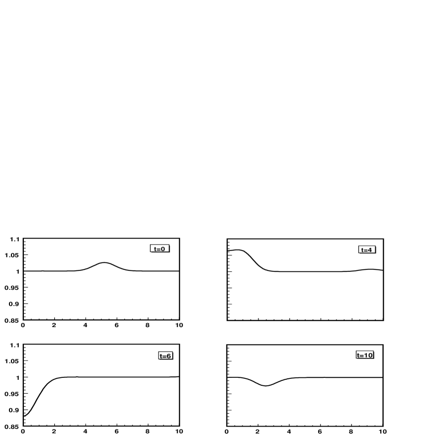
Figure 1 shows the evolution of the lapse function $\alpha$ near the origin. One can clearly see that the lapse remains perfectly smooth when the Gaussian pulse goes through the origin. The system can in fact evolve for very long times and the behavior at the origin remains well behaved.

V.2 Minkowski in axial symmetry using ADM

In this section we present a similar evolution to the one of the last Section, but done now with an axi-symmetric code using the ADM formulation. We again consider initial data corresponding to a trivial slice of Minkowski, so that the initial metric and extrinsic curvature have the form

$\displaystyle A$	$\displaystyle=$	$\displaystyle B=T=1\;,$	(95)
$\displaystyle C$	$\displaystyle=$	$\displaystyle C_{1}=C_{2}=0\;,$	(96)
$\displaystyle K_{A}$	$\displaystyle=$	$\displaystyle K_{B}=K_{T}=0\;,$	(97)
$\displaystyle K_{C}$	$\displaystyle=$	$\displaystyle K_{C_{1}}=K_{C_{2}}=0\;,$	(98)

which implies,

	$\displaystyle H$	$\displaystyle=$	$\displaystyle 1\;,\quad J=0\;,$		(100)
	$\displaystyle K_{H}$	$\displaystyle=$	$\displaystyle K_{J}=0\;,$		(101)

Again, we chose an initial non-trivial lapse profile which for simplicity is now centered at the origin:

\alpha(t=0)=1+R\exp\left[-\left(\frac{z}{\sigma_{z}}\right)^{2}-\left(\frac{\rho}{\sigma_{\rho}}\right)^{2}\right]\;.

(102)

For the particular simulation presented here we have taken $R=0.015$ , $\sigma_{\rho}=\sigma_{z}=2.5$ . We will again evolve the lapse using harmonic slicing, $f(\alpha)=1$ . For this simulation we have used a grid spacing of $\Delta\rho=\Delta z=0.125$ , with a Courant factor of $\Delta t/\Delta\rho=0.25$ . The outer boundaries are at $\rho=129,z=\pm 129$ . Furthermore, Kreiss-Oliger fourth order dissipation has been added for stability Gustafsson et al. (1995), whereby we modify a given variable $u$ in the new time-step by adding to its evolution equation

$\displaystyle\partial_{t}u_{i,j}$	$\displaystyle\rightarrow$	$\displaystyle\partial_{t}u_{i,j}-\frac{\epsilon}{\Delta\rho}\left(u_{i+2,j}-4u_{i-1,j}\right.$	(103)
		$\displaystyle\left.+6u_{i,j}-4u_{i-1,j}+u_{i-2,j}\right)$
		$\displaystyle-\frac{\epsilon}{\Delta z}\left(u_{i,j+2}-4u_{i,j+2}\right.$
		$\displaystyle\left.+6u_{i,j}-4u_{i,j-1}+u_{i,j-2}\right),$

where the indices $i,j$ refer to the grid points along the $\rho$ and $z$ directions. For this simulation the dissipation coefficients have been taken to be $\epsilon_{\rho}=\epsilon_{z}=0.04$ .

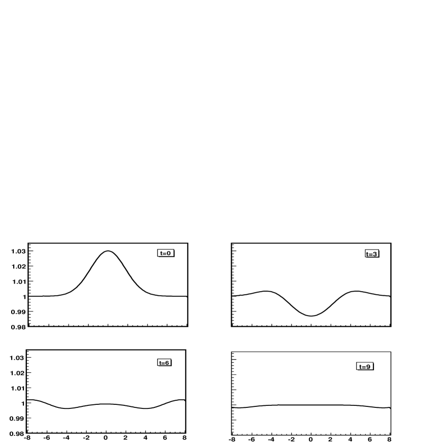
Figure 2 shows the evolution of lapse function $\alpha$ along the $\rho$ axis. Notice that again there is no problem at the axis of symmetry: The lapse evolves as a wave, goes through the origin, and finally returns to 1. The evolution time is only limited by the instabilities produced from the fact that ADM is not strongly hyperbolic.

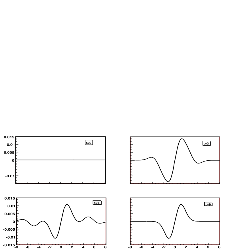
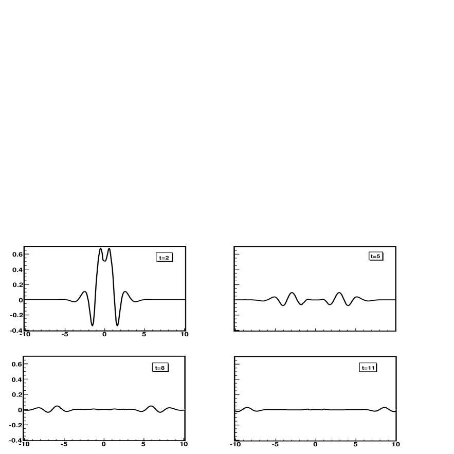
V.3 Minkowski in axial symmetry using a hyperbolic formulation

In our next example, we consider exactly the same situation as in the last Section but using now a hyperbolic formulation. As before, we have used a grid spacing of $\Delta\rho=\Delta z=0.125$ and a Courant factor of $\Delta t/\Delta\rho=0.25$ . Again, Kreiss-Oliger second order dissipation has been added for stability with dissipation coefficients $\epsilon_{\rho}=\epsilon_{z}=0.04$ .

Figures 3, 4 and 5 show the evolution of the lapse function $\alpha$ , the radial metric $A$ , and the variable $\Delta^{\rho}$ along the $\rho$ axis. We evolve the system until $50M$ and all variables remain well behaved on the axis.

V.4 Brill waves

For our last example we have considered a non-trivial Brill wave spacetime, which corresponds to strong non-linear gravitational waves in vacuum. The construction of such a spacetime starts by considering an axi-symmetric initial slice with a metric of the form

ds^{2}=\Psi^{4}\left[e^{2q}\left(d\rho^{2}+dz^{2}\right)+\rho^{2}d\phi^{2}\right]\;,

(104)

where both $q$ and $\Psi$ are functions of $(t,\rho,z)$ only. In order to solve for $\Psi$ , we first impose the condition of time symmetry, that is, $K_{ij}=0$ . This condition implies that the momentum constraints (4) are identically satisfied. We then choose a specific form for the function $q$ and solve the Hamiltonian constraint for $\Psi$ , which for the metric (104) becomes

\Delta_{\delta}\Psi+\frac{1}{4}\,\left(q_{,\rho\rho}+q_{,zz}\right)\Psi=0\;,

(105)

with $\Delta_{\delta}$ the flat space Laplacian. The function $q$ is quasi-arbitrary, and must only satisfy the following boundary conditions

$\displaystyle q\left\|{}_{\rho=0}\right.$	$\displaystyle=$	$\displaystyle 0\;,$	(106)
$\displaystyle\partial^{n}_{\rho}q\left\|{}_{\rho=0}\right.$	$\displaystyle=$	$\displaystyle 0\qquad\mbox{for odd $n$}\;,$	(107)
$\displaystyle q\left\|{}_{r\rightarrow\infty}\right.$	$\displaystyle=$	$\displaystyle O\left(r^{-2}\right)\;.$	(108)

Once a function $q$ has been chosen, all that is left for one to do is to solve the elliptic equation (105) numerically.

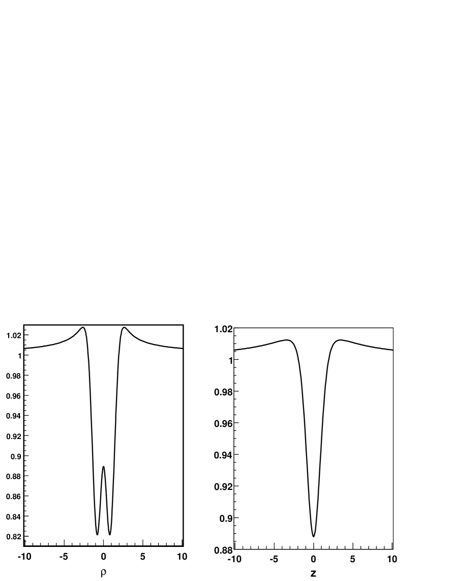
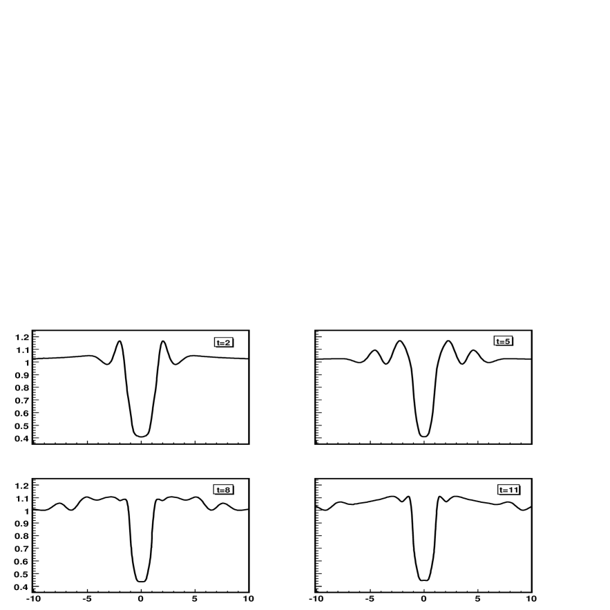
Different forms of the function $q$ have been used by different authors Eppley (1977); Holz et al. (1993). Here we will consider the one introduced by Holz and collaborators in Holz et al. (1993), which has the form

q=a\rho^{2}e^{-(\rho^{2}+z^{2})}\;,

(109)

with $a$ a constant that determines the initial amplitude of the wave (for small $a$ the waves disperse to infinity, while for large $a$ they can collapse to form a black hole). Figure 6 shows the value of $\Psi$ along the equator $z=0$ and axis $\rho=0$ obtained by solving equation (105) numerically for an amplitude of $a=2.0$ (small enough so that no black hole is formed, but large enough so that we are far from the linear regime).

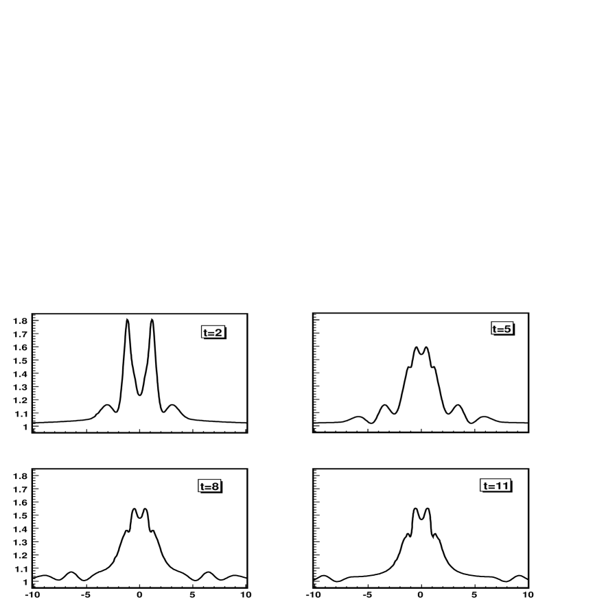
For the evolution of this initial data we have used a grid spacing of $\Delta\rho=\Delta z=0.125$ and a Courant factor of $\Delta t/\Delta\rho=0.2$ , with the outer boundaries located at $\rho=165,z=\pm 165$ . For the lapse evolution we use a 1+log slicing condition, which corresponds to a Bona-Masso (7) slicing with $f(\alpha)=2/\alpha$ . Again, Kreiss-Oliger second order dissipation has been added for stability.

Figures 7, 8 and 9 show the evolution of the extrinsic curvature component $K_{zz}$ , and the metric components $B$ and $T$ along the $\rho$ axis. Notice again that for this simulation there is no problem at the axis of symmetry in the evolution of the different geometric quantities.

VI Discussion

We have presented a regularization procedure for the numerical simulation of spacetimes with either spherical or axial symmetry following an idea of Rinne and Stewart Rinne and Stewart (2005). This procedure enforces both the parity conditions and the conditions arising from local flatness at the origin and the axis of symmetry. We paid particular attention to the fact that our regularization procedure is independent of the system of evolution equations chosen, explicitly showing this in the case of the ADM formulation, as well as a strongly hyperbolic formulation similar to that of Nagy, Ortiz and Reula Nagy et al. (2004) (slightly modified in order to have all the dynamical variables well defined in curvilinear coordinates).

We have also described numerical codes that follow such regularization procedure both in spherical and axial symmetry, and presented several examples clearly showing that all dynamical variables remain regular at the origin and axis of symmetry in each case (similar numerical experiments using the regularized Z4 system of Rinne and Stewart (2005); Rinne (2005) have also been carried out by Rinne and Stewart in Rinne (2005)). These results show that one can construct well behaved numerical codes in both spherical and axial symmetry that can allow the study of interesting astrophysical systems with quite modest computer resources by using symmetry adapted coordinate systems.

We conclude by mentioning that one can also construct regular codes using specialized gauge choices which can even allow one to reduce the number of independent components of the metric. Nevertheless, our interest here has been to find a regularization procedure that works in the most general case, while leaving the choice of gauge completely arbitrary.

Acknowledgements.

This work was supported in part by Dirección General de Estudios de Posgrado (DEGP), by CONACyT through grants 47201-F, 47209-F, and by DGAPA-UNAM through grant IN113907.

Appendix A Evolution Equation in the Spherical Case

In this appendix we give explicitly the evolution equations for the hyperbolic system presented in the section II.2 in order to show that all equations are manifestly regular. We only consider the case of spherical symetry, since in axi-symmetry the final equations are just too long to write down here (they have been calculated with Mathematica, and some of them are dozens of lines long). For the spherical case, the resulting system of evolution equations is, together with (47):

$\displaystyle\partial_{t}K_{H}$	$\displaystyle=$	$\displaystyle\frac{\alpha H^{3}}{2rA^{2}T^{2}}\,\left(\Delta^{r}H^{2}-F_{r}H-2D_{H}\right)+\frac{\alpha}{2A^{2}T^{2}}\Bigg{[}\frac{{D_{H}}^{2}}{4}\left({3H^{2}}-r^{2}J(A+9H)\right)+\frac{Ar^{4}{D_{J}}^{2}T}{4}$	(110)
	$\displaystyle+$	$\displaystyle H^{2}Jr^{2}\left(J+2K_{A}K_{H}-2rF_{r}J\right)+\left(A^{2}{D_{H}}T^{2}-rJ\left(r^{2}H^{3}J+r^{2}AHJT+A^{2}T^{2}\right)\right)\,{\Delta^{r}}$
	$\displaystyle+$	$\displaystyle rD_{H}J\left(5H^{2}+8r^{2}HJ+13r^{4}J^{2}\right)+r^{6}J^{3}\left(-2K_{A}{K_{H}}+3J\left(rF_{r}-5\right)\right)-A^{2}{F_{r}}^{2}T^{2}$
	$\displaystyle+$	$\displaystyle r^{2}D_{J}\left(AF-H^{2}J-5r^{5}J^{3}\right)+2H^{3}\left(J+2rF_{r}J+{K_{A}}\left({K_{T}}-r^{2}{K_{J}}\right)\right)-4A^{2}T^{2}\partial_{r}F_{r}$
	$\displaystyle-$	$\displaystyle 2r^{4}HJ^{2}\left(2J\left(rF_{r}+7\right)+K_{A}\left(K_{T}-r^{2}K_{J}\right)\right)+\frac{r^{4}HD_{J}}{2}\,\left(D_{J}H-36J^{2}r-5D_{J}Jr^{2}\right)$
	$\displaystyle+$	$\displaystyle\frac{1}{2}D_{H}D_{J}r^{2}\left(3H^{2}-2HJr^{2}+7J^{2}r^{4}\right)T^{2}+A^{3}T^{2}\partial_{r}\Delta^{r}-AT^{2}\partial_{r}{D_{H}}\Bigg{]}\,,$

$\displaystyle\partial_{t}K_{J}$	$\displaystyle=$	$\displaystyle\frac{\alpha H^{5}}{2rA^{2}T^{2}}\>\partial_{r}\left(\frac{\Delta^{r}}{r}\right)-\frac{\alpha H^{4}}{2rA^{2}T^{2}}\>\partial_{r}\left(\frac{F_{r}}{r}\right)+\frac{\alpha H^{2}D_{H}}{8r^{2}A^{2}T^{2}}\left(4F_{r}H-D_{H}\right)+\frac{\alpha H^{2}}{2rA^{2}T^{2}}$	(111)
	$\displaystyle\times$	$\displaystyle\left(-6HD_{J}+11JD_{H}-2HJF_{r}+3JH^{2}\Delta^{r}\right)+D_{H}^{2}\left(-5HJ+\frac{3J^{2}r^{2}}{2}\right)$
	$\displaystyle+$	$\displaystyle D_{H}\left(H^{2}\left(7D_{J}-2JF_{r}\right)+12HJ^{2}r-2HJ\left(D_{J}+Jr^{2}F_{r}\right)+14J^{3}r^{3}+J^{2}r^{4}\left(3D_{J}+2JF_{r}\right)\right)$
	$\displaystyle-$	$\displaystyle 4H^{3}K_{A}K_{J}+HJr^{2}\left(-5D_{J}^{2}r^{2}+4J^{2}\left(rF_{r}-13\right)+4Jr\left(-6D_{J}+K_{A}K_{J}r\right)\right)$
	$\displaystyle+$	$\displaystyle 4H^{2}\left(JK_{A}\left(K_{H}+K_{T}\right)-3JrD_{J}+J^{2}\left(2r^{2}F_{r}^{2}-9-\frac{D_{J}^{2}r^{2}}{4}\right)\right)-2AT^{2}\partial_{r}D_{J}$
	$\displaystyle-$	$\displaystyle J^{2}r^{4}\left(8JK_{A}\left(K_{H}+K_{T}\right)+12rJD_{J}-3D_{J}^{2}r^{2}+4J^{2}\left(rF_{r}\left(rF_{r}+1\right)+5\right)\right)$
	$\displaystyle+$	$\displaystyle 2\left(A^{2}D_{J}T^{2}+J^{2}r\left(-2Jr^{2}+T\right)\left(H^{2}+AT\right)\right)\Delta^{r}+2\left(2H^{2}J^{2}r^{2}-J^{4}r^{6}\right)\partial_{r}F_{r}$
	$\displaystyle+$	$\displaystyle 2J\left(-H^{2}\left(A+H\right)Jr^{2}+AJ^{3}r^{6}+AH^{2}T\right)\,\partial_{r}\Delta^{r}\,,$

$\displaystyle\partial_{t}\Delta^{r}$	$\displaystyle=$	$\displaystyle\frac{\alpha}{A^{3}T^{2}}\Bigg{[}2H^{2}r\left(6JK_{H}+AK_{J}\right)+12J^{3}r^{5}K_{H}-10AJ^{2}r^{5}K_{J}$	(112)
	$\displaystyle+$	$\displaystyle AF_{r}T\left(-AK_{J}r^{2}+K_{H}\left(A+2Jr^{2}\right)\right)+2D_{H}K_{A}T^{2}+2D_{J}K_{A}r^{2}T^{2}-A^{2}T\partial_{r}K_{H}$
	$\displaystyle-$	$\displaystyle 2H\left(J^{2}\left(-4K_{T}r^{3}+4K_{J}r^{5}\right)+AT\left(F_{r}K_{J}r^{2}+\partial_{r}K_{H}\right)\right)+A\left(A+2J\right)r^{2}T\partial_{r}K_{J}\Bigg{]}\,.$

Considering the results of Section III, we see that the above equations are manifestly regular at the origin.

References

Pretorius (2005) F. Pretorius, Phys. Rev. Lett. 95, 121101 (2005), eprint gr-qc/0507014.
Campanelli et al. (2006) M. Campanelli, C. O. Lousto, P. Marronetti, and Y. Zlochower, Phys. Rev. Lett. 96, 111101 (2006), eprint gr-qc/0511048.
Baker et al. (2006) J. G. Baker, J. Centrella, D.-I. Choi, M. Koppitz, and J. van Meter, Phys. Rev. Lett. 96, 111102 (2006), eprint gr-qc/0511103.
Bardeen and Piran (1983) J. Bardeen and T. Piran, Phys. Rep. 196, 205 (1983).
Abrahams and Evans (1993) A. M. Abrahams and C. R. Evans, Phys. Rev. Lett. 70, 2980 (1993).
Evans (1986) C. R. Evans, in Dynamical spacetimes and numerical relativity, edited by J. M. Centrella (Cambridge University Press, 1986), pp. 3–39.
Garfinkle and Duncan (2001) D. Garfinkle and G. C. Duncan, Phys. Rev. D63, 044011 (2001), eprint gr-qc/0006073.
Choptuik et al. (2003) M. W. Choptuik, E. W. Hirschmann, S. L. Liebling, and F. Pretorius, Class. Quant. Grav. 20, 1857 (2003), eprint gr-qc/0301006.
Bona et al. (2003) C. Bona, T. Ledvinka, C. Palenzuela, and M. Zacek, Phys. Rev. D67, 104005 (2003), eprint gr-qc/0302083.
Bona et al. (2004) C. Bona, T. Ledvinka, C. Palenzuela, and M. Zacek, Phys. Rev. D69, 064036 (2004), eprint gr-qc/0307067.
Rinne and Stewart (2005) O. Rinne and J. M. Stewart, Class. Quant. Grav. 22, 1143 (2005), eprint gr-qc/0502037.
Rinne (2005) O. Rinne (2005), eprint gr-qc/0601064.
Alcubierre et al. (2001) M. Alcubierre, S. Brandt, B. Brügmann, D. Holz, E. Seidel, R. Takahashi, and J. Thornburg, Int. J. Mod. Phys. D 10, 273 (2001), gr-qc/9908012.
Alcubierre and González (2005) M. Alcubierre and J. González, Comp. Phys. Comm. 167, 76 (2005), gr-qc/0401113.
Nagy et al. (2004) G. Nagy, O. E. Ortiz, and O. A. Reula, Phys. Rev. D70, 044012 (2004), eprint gr-qc/0402123.
Alcubierre et al. (2005) M. Alcubierre, A. Corichi, J. González, D. Nuñez, B. Reimann, and M. Salgado, Phys. Rev. D 72, 124018 (2005), gr-qc/0507007.
Bona et al. (1995) C. Bona, J. Massó, E. Seidel, and J. Stela, Phys. Rev. Lett. 75, 600 (1995), gr-qc/9412071.
Gustafsson et al. (1995) B. Gustafsson, H. Kreiss, and J. Oliger, Time dependent problems and difference methods (Wiley, New York, 1995).
Eppley (1977) K. Eppley, Phys. Rev. D 16, 1609 (1977).
Holz et al. (1993) D. Holz, W. Miller, M. Wakano, and J. Wheeler, in Directions in General Relativity: Proceedings of the 1993 International Symposium, Maryland; Papers in honor of Di eter Brill, edited by B. Hu and T. Jacobson (Cambridge University Press, Cambridge, England, 1993).