Reinforcement Learning for Selective Key Applications in Power Systems: Recent Advances and Future Challenges
Abstract
With large-scale integration of renewable generation and distributed energy resources, modern power systems are confronted with new operational challenges, such as growing complexity, increasing uncertainty, and aggravating volatility. Meanwhile, more and more data are becoming available owing to the widespread deployment of smart meters, smart sensors, and upgraded communication networks. As a result, data-driven control techniques, especially reinforcement learning (RL), have attracted surging attention in recent years. This paper provides a comprehensive review of various RL techniques and how they can be applied to decision-making and control in power systems. In particular, we select three key applications, i.e., frequency regulation, voltage control, and energy management, as examples to illustrate RL-based models and solutions. We then present the critical issues in the application of RL, i.e., safety, robustness, scalability, and data. Several potential future directions are discussed as well.
Index Terms:
Frequency regulation, voltage control, energy management, reinforcement learning, smart grid.Nomenclature
-A Notations
- ,
-
Action space, action.
-
, the set of lines connecting buses.
-
Expected total discounted reward.
-
, the set of buses in a power network or the set of agents.
-
Neural network with input and parameter .
-
Observation.
-
Transition probability.
-
-function (or -value) under policy .
-
Reward.
- ,
-
State space, state.
-
, the discrete time horizon.
-
Discounting factor.
-
The set of probability distributions over set .
-
The time interval in .
- ,
-
Policy, optimal policy.
-B Abbreviations
- A3C
-
Asynchronous Advantaged Actor Critic.
- ACE
-
Area Control Error.
- AMI
-
Advanced Metering Infrastructure.
- ANN
-
Artificial Neural Network.
- DDPG
-
Deep Deterministic Policy Gradient.
- DER
-
Distributed Energy Resource.
- DP
-
Dynamic Programming.
- (D)RL
-
(Deep) Reinforcement Learning.
- DQN
-
Deep Network.
- EMS
-
Energy Management System.
- EV
-
Electric Vehicle.
- FR
-
Frequency Regulation.
- HVAC
-
Heating, Ventilation, and Air Conditioning.
- IES
-
Integrated Energy System.
- LSPI
-
Least-Squares Policy Iteration.
- LSTM
-
Long-Short Term Memory.
- MDP
-
Markov Decision Process.
- OLTC
-
On-Load Tap Changing Transformer.
- OPF
-
Optimal Power Flow.
- PMU
-
Phasor Measurement Unit.
- PV
-
Photovoltaic.
- SAC
-
Soft Actor Critic.
- SCADA
-
Supervisory Control and Data Acquisition.
- SVC
-
Static Var (Reactive Power) Compensator.
- TD
-
Temporal Difference.
- UCRL
-
Upper Confidence Reinforcement Learning.
I Introduction
Electric power systems are undergoing an architectural transformation to become more sustainable, distributed, dynamic, intelligent, and open. On the one hand, the proliferation of renewable generation and distributed energy resources (DERs), including solar energy, wind power, energy storage, responsive demands, electric vehicles (EVs), etc., creates severe operational challenges. On the other hand, the deployment of information, communication, and computing technologies throughout the electric system, such as phasor measurement units (PMUs), advanced metering infrastructures (AMIs), and wide area monitoring systems (WAMS) [1], has been growing rapidly in recent decades. It evolves traditional power systems towards smart grids and offers an unprecedented opportunity to overcome these challenges through real-time data-driven monitoring and control at scale. This will require new advanced decision-making and control techniques to manage
-
1)
Growing complexity. The deployment of massive DERs and the interconnection of regional power grids dramatically increase system operation complexity and make it difficult to obtain accurate system (dynamical) models.
-
2)
Increasing uncertainty. The rapid growth of renewable generation and responsive loads significantly increases uncertainty, especially when human users are involved, jeopardizing predictions and system reliability.
-
3)
Aggravating volatility. The high penetration of power electronics converter-interfaced devices reduces system inertia, which leads to faster dynamics and necessitates advanced controllers with online adaptivity.
In particular, reinforcement learning (RL) [2], a prominent machine learning paradigm concerned with how agents take sequential actions in an uncertain interactive environment and learn from the feedback to optimize a specific performance, can play an important role in overcoming these challenges. Leveraging artificial neural networks (ANNs) for function approximation, deep RL (DRL) [3] is further developed to solve large-scale online decision problems. The most appealing virtue of (D)RL is its model-free nature, i.e., it makes decisions without explicitly estimating the underlying models. Hence, (D)RL has the potential to capture hard-to-model dynamics and could outperform model-based methods in highly complex tasks. Moreover, the data-driven nature of (D)RL allows it to adapt to real-time observations and perform well in uncertain dynamical environments. Over the past decade, (D)RL has achieved great success in a broad spectrum of applications, such as playing games [4], robotics [5], autonomous driving [6], clinical trials [7], etc.
Meanwhile, the application of RL in power system operation and control has attracted surging attention [8, 9, 10, 11]. RL-based decision-making mechanisms are envisioned to compensate for the limitations of existing model-based approaches and thus are promising to address the emerging challenges described above. This paper provides a review and survey on RL-based decision-making in smart grids. We will introduce various RL terminologies, exemplify how to apply RL to power systems, and discuss critical issues in their application. Compared with recent review articles [8, 9, 10, 11] on this subject, the main merits of this paper include
-
1)
We present a comprehensive and structural overview of the RL methodology, from basic concepts and theoretical fundamentals to state-of-the-art RL techniques.
-
2)
Three key applications are selected as examples to illustrate the overall procedure of applying RL to the control and decision-making in power systems, from modeling, solution, to numerical implementation.
-
3)
We discuss the critical challenges and future directions for applying RL to power system problems in depth.
In the rest of this paper, Section II presents a comprehensive overview of the RL fundamentals and the state-of-the-art RL techniques. Section III describes the application of RL to three critical power system problems, i.e., frequency regulation, voltage control, and energy management, where paradigmatic mathematical models are provided for illustration. Section IV summarizes the key issues of safety, robustness, scalability, and data, and then discusses several potential future directions. Lastly, we conclude in Section V.
II Preliminaries on Reinforcement Learning
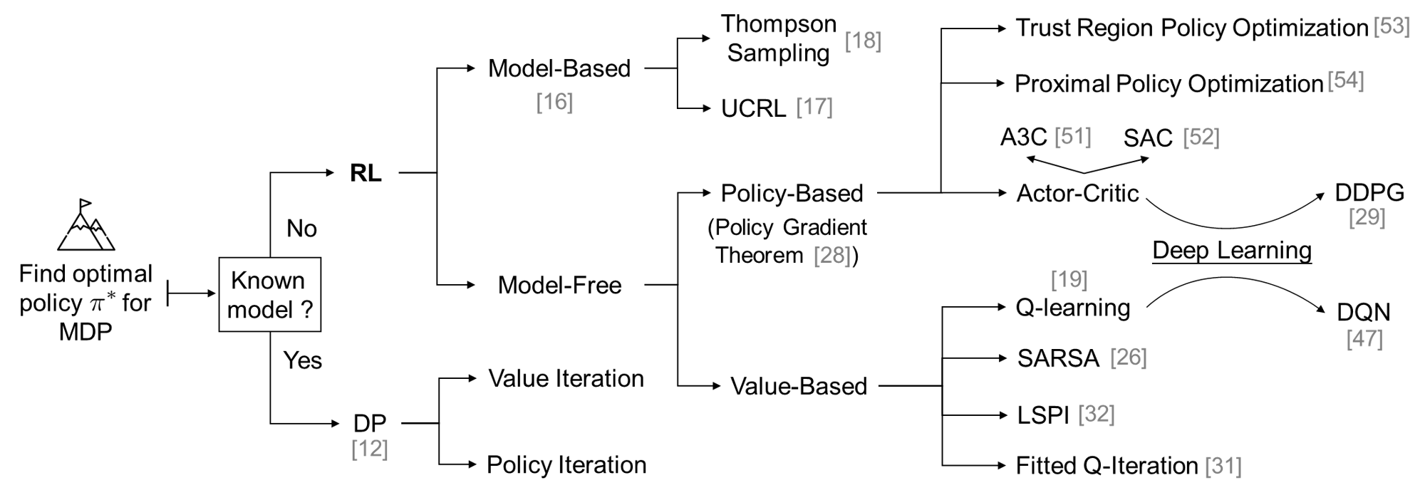
This section provides a comprehensive overview of the RL methodology. First, we set up the RL problem formulation and key concepts, such as -function and Bellman (Optimality) Equation. Then two categories of classical RL algorithms, i.e., value-based and policy-based, are introduced. With these fundamentals in place, we next present several state-of-the-art RL techniques, including DRL, deterministic policy gradient, modern actor-critic methods, multi-agent RL, etc. The overall structure of RL methodology with related literature is illustrated in Fig. 1.
II-A Fundamentals of Reinforcement Learning
RL is a branch of machine learning concerned with how an agent makes sequential decisions in an uncertain environment to maximize the cumulative reward. Mathematically, the decision-making problem is modeled as a Markov Decision Process (MDP), which is defined by state space , action space , the transition probability function that maps a state-action pair to a distribution on the state space, and lastly the reward function 111 A generic reward function is given by where the next state is also included as an argument, but there is no essential difference between the case with and the case with in algorithms and results. By marginalizing over next states according to the transition function , one can simply convert to [2].. The state space and action space can be either discrete or continuous. To simplify discussion, we focus on the discrete case below.
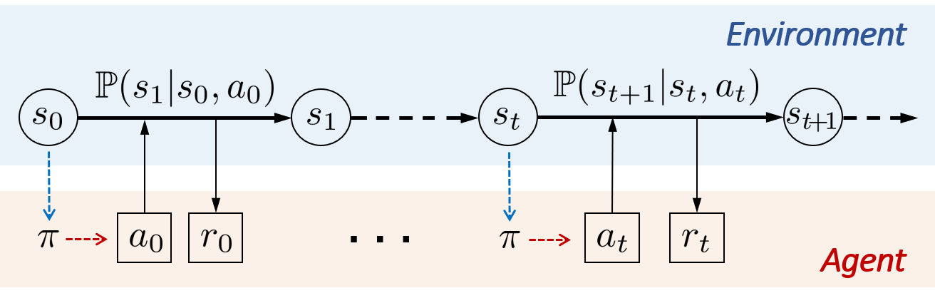
As illustrated in Fig. 2, in an MDP setting, the environment starts with an initial state . At each time , given current state , the agent chooses action and receives reward that depends on the current state-action pair , after which the next state is randomly generated from the transition probability . A policy for the agent is a map from the state to a distribution on the action space , which rules what action to take given a certain state .222 is a stochastic policy, and it becomes a deterministic policy when the probability distribution is a singleton for all . The agent aims to find an optimal policy (may not be unique) that maximizes the expected infinite horizon discounted reward :
| (1) |
where the first expectation means that is drawn from an initial state distribution , and the second expectation means that the action is taken according to the policy . Parameter is the discounting factor that penalizes the rewards in the future.
In the MDP framework, the so-called “model” specifically refers to the reward function and the transition probability . Accordingly, it leads to two different problem settings:
-
•
When the model is known, one can directly solve for an optimal policy by Dynamic Programming (DP) [12].
-
•
When the model is unknown, the agent learns an optimal policy based on the past observations from interacting with the environment, which is the problem of RL.
Since DP lays the foundation for RL algorithms, we first consider the case with a known model and introduce the basic ideas of finding an optimal policy with respect to (1). The crux is the concept of -function together with the Bellman Equation. The -function for a given policy is defined as
| (2) |
which is the expected cumulative reward when the initial state is , the initial action is , and all the subsequent actions are chosen according to policy . The -function satisfies the following Bellman Equation: ,
| (3) |
where the expectation denotes that the next state is drawn from , and the next action is drawn from . Here, it is helpful to think of the -function as a large table or vector filled with -values . The Bellman Equation (3) indicates a recursive relation that each -value equals the immediate reward plus the discounted future value. Computing the -function for a given policy is called policy evaluation, which can be done by simply solving a set of linear equations when the model, i.e., and , is known.
The -function associated with an optimal policy for (1) is called an optimal -function and denoted as . The key to find is that the optimal -function must be the unique solution to the Bellman Optimality Equation (4): ,
| (4) |
Interested readers are referred to textbook [12, Sec. 1.2] on why this is true. Based on the Bellman Optimality Equation (4), the optimal -function and an optimal policy can be solved using DP or linear programming [12, Sec. 2.4]. In particular, policy iteration and value iteration are two classic DP algorithms. See [2, Chapter 4] for details.
Remark 1.
(Modeling Issues with MDP). MDP is a generic framework to model sequential decision-making problems and is the basis for RL algorithms. However, several issues deserve attention when modeling power system control problems in the MDP framework.
-
1)
At the heart of MDP is the Markov property that the distribution of future states depends only on the present state and action, i.e., . In other words, given the present, the future does not depend on the past. Then for a specific control problem, one needs to check whether the choices of state and action satisfy the Markov property. A general guideline is to include all necessary known information in the enlarged state, known as state augmentation [12], to maintain the Markov property, however, at the cost of complexity.
-
2)
Most classical MDP theories and RL algorithms are based on discrete-time transitions, but many power system control problems follow continuous-time dynamics, such as frequency regulation. To fit the MDP framework, continuous-time dynamics are generally discretized with a proper temporal resolution, which is a common issue for digital control systems, and there are well-established frameworks to deal with it. Besides, there are RL variants that are built directly on continuous-time dynamics, such as integral RL [13].
-
3)
Many MDP/RL methods assume time-homogeneous state transitions and rewards. But in power systems, there are various time-varying exogenous inputs and disturbances, making the state transitions not time-homogeneous. This is an important problem that has not been adequately explored in the existing power literature and needs further study. Nonstationary MDP [14] and related RL algorithms [15] could be the potential directions.
In addition, the issues of continuous state/action spaces and partial observability for MDP modeling will be discussed later.
II-B Classical Reinforcement Learning Algorithms
This subsection considers the RL setting when the environment model is unknown, and presents classical RL algorithms for finding the optimal policy . As shown in Fig. 1, RL algorithms can be divided into two categories, i.e., model-based and model-free. “Model-based” refers to the RL algorithms that explicitly estimate and online update an environment model from past observations and make decisions based on this model [16], such as upper confidence RL (UCRL) [17] and Thompson sampling [18]. In contrast, “model-free” means that the RL algorithms directly search for optimal policies without estimating the environment model. Model-free RL algorithms are mainly categorized into two types, i.e., value-based and policy-based. Generally, value-based methods are preferred for modest-scale RL problems with finite state/action space as they do not assume a policy class and have a strong convergence guarantee. The convergence of value-based methods to an optimal -function in the tabular setting (without function approximation) was proven back in the 1990s [19]. In contrast, policy-based methods are more efficient for problems with high dimensions or continuous action/state space. But they are known to suffer from various convergence issues, e.g., local optimum, high variance, etc. The convergence of policy-based methods with restricted policy classes to the global optimum has been shown in a recent work [20] under the tabular policy parameterization.
Remark 2.
(Exploration vs. Exploitation). A fundamental problem faced by RL algorithms is the dilemma between exploration and exploitation. Good performance requires taking actions adaptively to strike an effective balance between 1) exploring poorly-understood actions to gather new information that may improve future reward, and 2) exploiting what is known for decision-making to maximize immediate reward. Generally, it is natural to achieve exploitation with the goal of reward maximization, while different RL algorithms encourage exploration in different ways. For value-based RL algorithms, -greedy is commonly used with a probability of to explore random actions. In policy-based methods, exploration is usually achieved by injecting random perturbation to the actions, adopting a stochastic policy, or adding an entropy term to the objective, etc.
Before presenting classical RL methods, we introduce a key algorithm, Temporal-Difference (TD) learning [21], for policy evaluation when the model is unknown. TD learning is central to both value-based and policy-based RL algorithms. It learns the -function for a given policy from episodes of experience. Here, an “episode” refers to a state-action-reward trajectory over time until terminated. Specifically, TD learning maintains a -function for all state-action pairs and updates it upon a new observation by
| (5) | ||||
where is the step size. Readers might observe that the second term in (5) is very similar to the Bellman Equation (3), which is exactly the rationale behind TD learning. Essentially, TD learning (5) is a stochastic approximation scheme for solving the Bellman Equation (3) [22], and can be shown to converge to the true under mild assumptions [21, 23].
1) Value-based RL algorithms directly learn the optimal -function , and the optimal (deterministic) policy is a byproduct that can be retrieved by acting greedily, i.e., . Among many, -learning [24, 19] is perhaps the most popular value-based RL algorithm. Similar to TD-learning, -learning maintains a -function and updates it towards the optimal -function based on episodes of experience. Specifically, at each time , given current state , the agent chooses action according to a certain behavior policy.333Such a behavior policy, also called exploratory policy, can be arbitrary as long as it visits all the states and actions sufficiently often. Upon observing the outcome , -learning updates the -function by
| (6) | ||||
The rationale behind (6) is that the -learning algorithm (6) is essentially a stochastic approximation scheme for solving the Bellman Optimality Equation (4), and one can show the convergence to under mild assumptions [19, 25].
SARSA444In some literature, SARSA is also called -learning. [26] is another classical value-based RL algorithm, whose name comes from the experience sequence . SARSA is actually an on-policy variant of -learning. The major difference is that SARSA takes actions according to the target policy (typically -greedy based on the current -function) rather than any arbitrary behavior policy in -learning. The following remark distinguishes and compares “on-policy” and “off-policy” RL algorithms.
Remark 3.
(On-Policy vs. Off-Policy). On-policy RL methods continuously improve a policy (called target policy) and implement this policy to generate episodes for algorithm training. In contrast, off-policy RL methods learn a target policy based on the episodes that are generated by following a different policy (called behavior policy) rather than the target policy itself. In short, “on” and “off” indicate whether the training samples are generated by following the target policy or not. For example, -learning is an off-policy RL method as the episodes used in training can be produced by any policies, and the actor-critic algorithm described below is on-policy.555There are also off-policy variants of the actor-critic algorithm, e.g., [27]. For power system applications, control policies that are not well-trained are generally not allowed to be implemented in real-world power grids for the sake of safety. Thus off-policy RL is preferred when high-fidelity simulators are unavailable since it can learn from the vast amount of operational data generated by incumbent controllers. Off-policy RL is also relatively easy to provide a safety guarantee due to the flexibility in choosing the behavior policies, but it is known to suffer from slower convergence and higher sample complexity.
2) Policy-based RL algorithms restrict the optimal policy search to a policy class that is parameterized as with the parameter . With this parameterization, the objective (1) can be rewritten as a function of the policy parameter, i.e., , and the RL problem is reformulated as an optimization problem (7) that aims to find the optimal :
| (7) |
To solve (7), a straightforward idea is to employ the gradient ascent method, i.e., , where is the step size. However, computing the gradient was supposed to be intrinsically hard as the environment model is unknown. Policy Gradient Theorem [28] is a big breakthrough in addressing the gradient computation issue. This theorem shows that the policy gradient can be simply expressed as
| (8) |
Here, is the on-policy state distribution [2, Chapter 9.2], which denotes the fraction of time steps spent in each state . Equation (8) is for a stochastic policy , while the version of policy gradient theorem for a deterministic policy [29] will be discussed later.
The policy gradient theorem provides a highway to estimate the gradient , which lays the foundation for policy-based RL algorithms. In particular, the actor-critic algorithm is a prominent and widely used architecture based on policy gradient. It comprises two eponymous components: 1) the “critic” is to estimate the -function , and 2) the “actor” conducts the gradient ascent based on (8). The following iterative scheme is an illustrative actor-critic example:
-
1)
Given state , take action , then observe the reward and next state ;
-
2)
(Critic) Update -function by TD learning;
-
3)
(Actor) Update policy parameter by
(9) -
4)
. Go to step 1) and repeat.
There are many actor-critic variants with different implementation manners, e.g., how is sampled from , how -function is updated, etc. See [2, Chapter 13] for more details.
We emphasize that the algorithms introduced above are far from complete. In the next subsections, we will introduce the state-of-the-art modern (D)RL techniques that are widely used in complex control tasks, especially for power system applications. At last, we close this subsection with the following two remarks on different RL settings.
Remark 4.
(Online RL vs. Batch RL). The algorithms introduced above are referred to as “online RL” that takes actions and updates the policies simultaneously. In contrast, there is another type of RL called “batch RL” [30], which decouples the sample data collection and policy training. Precisely, given a set of experience episodes generated by following any arbitrary behavior policies, batch RL fits the optimal -function or optimizes the target policy entirely based on this fixed sample dataset. Some classical batch RL algorithms include Fitted -Iteration [31], Least-Squares Policy Iteration (LSPI) [32], etc. For example, given a batch of transition experiences , Fitted -Iteration, which is seen as the batch version of -learning, aims to fit a parameterized -function by iterating the following two steps:
-
1)
Create the target -value for each sample in by
-
2)
Apply regression approaches to fit a new based on the training dataset .
The crucial advantages of batch RL lie in the stability and data-efficiency of the learning process by making the best use of the available sample datasets. However, because of relying entirely on a given dataset, the lack of exploration is one of the major problems of batch RL. To encourage exploration, batch RL typically iterates between exploratory sample collection and policy learning prior to application. Besides, pure batch RL, also referred to as “offline RL” [33], has attracted increasing recent attention, which completely ignores the exploration issue and aims to learn policies fully based on a static dataset with no online interaction. Offline RL assumes a sufficiently large and diverse dataset that adequately covers high-reward transitions for learning good policies and turns the RL problem into a supervised machine learning problem. See [34] for a tutorial of offline RL.
Remark 5.
(Passive RL, Active RL, and Inverse RL). The terminology “passive RL” typically refers to the RL setting where the agent acts by following a fixed policy and aims to learn how good this policy is from observations. It is analogous to the policy evaluation task, and TD learning is one of the representative algorithms of passive RL. In contrast, “active RL” allows the agent to update policies with the goal of finding an optimal policy, which is basically the standard RL setting that we described above. However, in some references, e.g., [35, 36], “active RL” has a completely different meaning and refers to the RL variant where the agent does not observe the reward unless it pays a query cost to account for the difficulty of collecting reward feedback. Thus, the agent chooses both an action and whether to observe the reward at each time. Another interesting RL variant is “inverse RL” [37, 38], in which the state-action sequence of an (expert) agent is given, and the task is to infer the reward function that this agent seeks to maximize. Inverse RL is motivated by various practical applications where the reward engineering is complex or expensive and one can observe an expert demonstrating the task to learn how to perform, e.g., autonomous driving.
II-C Fundamentals of Deep Learning
This subsection presents the fundamentals of deep learning to set the stage for the introduction of DRL. Deep learning refers to the machine learning technique that models with multi-layer ANNs. The history of ANNs dates back to 1940s [39], and it has received tremendous interests in the recent decade due to the booming of data technology and computing power, which allows efficient training of wider and deeper ANNs. Essentially, an ANN is an universal parameterized mapping from the input features to the outputs with the parameters . As illustrated in Fig. 3, an input feature vector is taken in by the input layer, then is processed through a series of hidden layers, and results in the output vector . Each hidden layer consists of a number of neurons that are the activation functions, e.g. linear, ReLU, or sigmoid [40]. Based on a sample dataset , the parameter can be optimized via regression. A landmark in training ANNs is the discovery of the back-propagation method, which offers an efficient way to compute the gradient of the loss function over [41]. Nevertheless, it is pretty tricky to train large-scale ANNs in practice, and article [41] provides an overview of the optimization algorithms and theory for training ANNs. Three typical classes of ANNs with different architectures are introduced below. See book [42] for details.
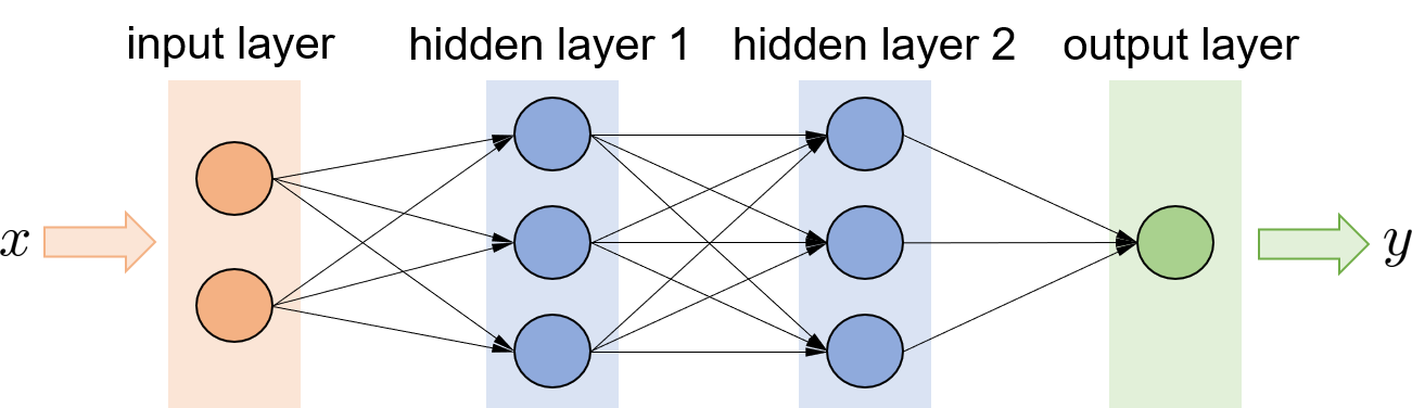
1) Convolutional Neural Networks (CNNs) are in the architecture of feed-forward neural networks (as shown in Fig. 3) and specialize in pattern detection, which are powerful for image analysis and computer vision tasks. The convolutional hidden layers are the basis at the heart of a CNN. Each neuron in a convolutional layer defines a small filter (or kernel) matrix of low dimension (e.g., ) and convolves with the input matrix of relatively high dimension, which leads to the output matrix . Here, denotes the convolution operator666Specifically, the convolution operation is performed by sliding the filter matrix across the input matrix and computing the corresponding element-wise multiplications, so that each element in matrix is the sum of the element-wise multiplications between and the associated sub-matrix of . See [42, Chapter 9] for a detailed definition of convolution., and the output is referred to as the feature map that is passed to the next layer. Besides, pooling layers are commonly used to reduce the dimension of the representation with the max or average pooling.
2) Recurrent Neural Networks (RNNs) specialize in processing long sequential inputs and tackling tasks with context spreading over time by leveraging a recurrent structure. Hence, RNNs achieve great success in the applications such as speech recognition and machine translation. RNNs process an input sequence one element at a time, and maintain in their hidden units a state vector that implicitly contains historical information about the past elements. Interestingly, the recurrence of RNNs is analogous to a dynamical system [42] and can be expressed as
| (10) |
where and are the input and output of the neural network at time step , and is the parameter for training. denotes the state stored in the hidden units at step and will be passed to the processing at step . In this way, implicitly covers all historical input information . Among many variants, long-short term memory (LSTM) network [44] is a special type of RNNs that excels at handling long-term dependencies and outperforms conventional RNNs by using special memory cells and gates.
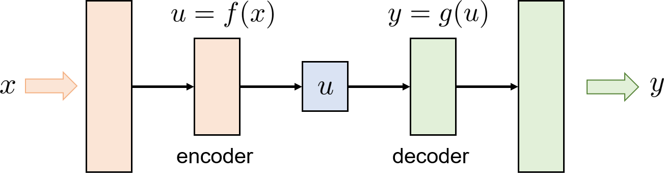
3) Autoencoders [45] are used to obtain a low-dimensional representation of high-dimensional inputs, which is similar to, but more general than, principal components analysis (PCA). As illustrated in Fig. 4, an autoencoder is in an hourglass-shape feed-forward network structure and consists of a encoder function and a decoder function . In particular, an autoencoder is trained to learn an approximation function with the loss function that penalizes the dissimilarity between the input and output . The bottleneck layer has a much smaller amount of neurons, and thus it is forced to form a compressed representation of the input .
II-D Deep Reinforcement Learning
For many practical problems, the state and action spaces are large or continuous, together with complex system dynamics. As a result, it is intractable for value-based RL to compute or store a gigantic -value table for all state-action pairs. To deal with this issue, function approximation methods are developed to approximate the -function with some parameterized function classes, such as linear function or polynomial function. As for policy-based RL, finding a capable policy class to achieve optimal control is also nontrivial in high-dimensional complex tasks. Driven by the advances of deep learning, DRL that leverages ANNs for function approximation or policy parameterization is becoming increasingly popular. Precisely, DRL can use ANNs to 1) approximate the -function with a -network , and 2) parameterize the policy with the policy network .
1) -Function Approximation. -network can be used to approximate the -function in TD learning (5) and -learning (6). For TD learning, the parameter is updated by
| (11) | ||||
where the gradient can be calculated efficiently using the back-propagation method. As for -learning, it is known that adopting a nonlinear function, such as an ANN, for approximation may cause instability and divergence issues in the training process. To this end, Deep -Network (DQN) [47] is developed and greatly improves the training stability of -learning with the following two tricks:
Experience Replay. Instead of performing on consecutive episodes, a widely used trick is to store all transition experiences in a database called “replay buffer”. At each step, a batch of transition experiences is randomly sampled from the replay buffer for -learning update. This can enhance the data efficiency by recycling previous experiences and reduce the variance of learning updates. More importantly, sampling uniformly from the replay buffer breaks the temporal correlations that jeopardize the training process, and thus improves the stability and convergence of -learning.
Target Network. The other trick is the introduction of the target network with parameter , which is a clone of the -network . Its parameter is kept frozen and is only updated periodically. Specifically, with a batch of transition experiences sampled from the replay buffer, the -network is updated by solving
| (12) |
The optimization (12) can be viewed as finding an optimal -network that approximately solves the Bellman Optimality Equation (4). The critical difference is that the target network with parameter instead of is used to compute the maximization over in (12). After a fixed number of updates above, the target network is renewed by replacing with the latest learned . This trick can mitigate the training instability as the short-term oscillations are circumvented. See [48] for more details.
In addition, there are several notable variants of DQN that further improve the performance, such as double DQN [49] and dueling DQN [50]. Particularly, double DQN is proposed to tackle the overestimation issue of the action values in DQN by learning two sets of -functions; one -function is used to select the action, and the other is used to determine its value. Dueling DQN proposes a dueling network architecture that separately estimates the state value function and the state-dependent action advantage function , which are then combined to determine the -value. The main benefit of this factoring is to generalize learning across actions without imposing any change to the underlying RL algorithm [50].
2) Policy Parameterization. Due to the powerful generalization capability, ANNs are widely used to parameterize control policies, especially when the state and action spaces are continuous. The resultant policy network takes states as the input and outputs the probability of action selection. In actor-critic methods, it is common to adopt both the -network and the policy network simultaneously, where the “actor” updates according to (9) and the “critic” updates according to (11). The back-propagation method [41] can be applied to efficiently compute the gradient of ANNs.
When function approximation is adopted, the theoretical analysis on both value-based and policy-based RL methods is little and generally limited to the linear function approximation. Besides, one problem that hinders the use of value-based methods for large or continuous action space is the difficulty of performing the maximization step. For example, when deep ANNs are used to approximate the -function, it is not easy to solve for the optimal action due to the nonlinear and complex formulation of .
II-E Other Modern Reinforcement Learning Techniques
This subsection summarizes several state-of-the-art modern RL techniques that are widely used in complex tasks.
II-E1 Deterministic Policy Gradient
The RL algorithms described above focus on stochastic policies , while deterministic policies are more desirable for many real-world control problems with continuous state and action spaces. On the one hand, since most incumbent controllers in physical systems, such as PID control and robust control, are all deterministic, deterministic policies are better matched to the practical control architectures, e.g., in power system applications. On the other hand, a deterministic policy is more sample-efficient as its policy gradient only integrates over the state space. In contrast, a stochastic policy gradient integrates over both state and action spaces [29]. Similar to the stochastic case, there is a Deterministic Policy Gradient Theorem [29] showing that the policy gradient with respect to a deterministic policy can be simply expressed as
| (13) |
Correspondingly, the “actor” in the actor-critic algorithm can update the parameter by
| (14) |
One major issue regarding a deterministic policy is the lack of exploration due to the determinacy of action selection. A common way to encourage exploration is to perturb a deterministic policy with exploratory noises, e.g., adding a Gaussian noise to the policy with .
II-E2 Modern Actor-Critic Methods
Although achieving great success in many complex tasks, the actor-critic methods are known to suffer from various problems, such as high variance, slow convergence, local optimum, etc. Therefore, many variants have been developed to improve the performance of actor-critic, and we list some of them below.
Advantaged Actor-Critic [2, Chapter 13.4]: The advantage function, , i.e., the -function subtracted by a baseline, is introduced to replace in the “actor” update, e.g., (9). One common choice for the baseline is an estimate of the state value function . This modification can significantly reduce the variance of the policy gradient estimate without changing the expectation.
Asynchronous Actor-Critic [51] presents an asynchronous variant with parallel training to enhance sample efficiency and training stability. In this method, multiple actors are trained in parallel with different exploration polices, then the global parameters get updated based on all the learning results and synchronized to each actor.
II-E3 Trust Region/Proximal Policy Optimization
To improve the training stability of policy-based RL algorithms, reference [53] proposes the Trust Region Policy Optimization (TRPO) algorithm, which enforces a trust region constraint (15b). It indicates that the KL-divergence between the old and new policies should not be larger than a given threshold . Denote as the probability ratio between the new policy and the old policy with . Then, TRPO aims to solve the constrained optimization (15):
| (15a) | ||||
| s.t. | (15b) | |||
where is an estimation of the advantage function. However, TRPO is hard to implement. To this end, work [54] proposes Proximal Policy Optimization (PPO) methods, which achieve the benefits of TRPO with simpler implementation and better empirical sample complexity. Specifically, PPO simplifies the policy optimization as (16):
| (16) |
where is a hyperparameter, e.g., , and the clip function enforces to stay within the interval . The “” of the clipped and unclipped objectives is taken to eliminate the incentive for moving outside of the interval to prevent big updates of .
II-E4 Multi-Agent RL
Many power system control tasks involve the coordination over multiple agents. For example, in frequency regulation, each generator can be treated as an individual agent that makes its own generation decisions, while the frequency dynamics are jointly determined by all power injections. It motivates the multi-agent RL framework, which considers a set of agents interacting with the same environment and sharing a common state . At each time , each agent takes its own action given the current state , and receives the reward , then the system state evolves to based on . Multi-agent RL is an active and challenging research area with many unsolved problems. An overview on related theories and algorithms is provided in [55]. In particular, the decentralized (distributed) multi-agent RL attracts a great deal of attention for power system applications. A popular variant is that each agent adopts a local policy with its parameter , which determines the action based on local observation (e.g., local voltage or frequency of bus ). This method allows for decentralized implementation as the policy for each agent only needs local observations, but it still requires centralized training since the system state transition relies on all agents’ actions. Multi-agent RL methods with distributed training are still under research and development.
Remark 6.
Although the RL techniques above are discussed separately, they can be integrated for a single problem to achieve all the benefits. For instance, one may apply the multi-agent actor-critic framework with deterministic policies, adopt ANNs to parameterize the -function and the policy, and use the advantage function for actor update. Accordingly, the resultant algorithm is usually named after the combination of key words, e.g., deep deterministic policy gradient (DDPG), asynchronous advantaged actor-critic (A3C), etc.
III Selective Applications of RL in Power Systems
Throughout the past decades, tremendous efforts have been devoted to improving the modeling of power systems. Schemes based on (optimal) power flow techniques and precise modeling of various electric facilities are standard for the control and optimization of power systems. However, the large-scale integration of renewable generation and DERs significantly aggravates the complexity, uncertainty, and volatility. It becomes increasingly arduous to obtain accurate system models and power injection predictions, challenging the traditional model-based approaches. Hence, model-free RL-based methods become an appealing complement. As illustrated in Fig. 5, the RL-based schemes relieve the need for accurate system models and learn control policies based on data collected from actual system operation or high-fidelity simulators, when the underlying physical models and dynamics are regarded as the unknown environment.

For power systems, frequency level and voltage profile are two of the most critical indicators of system operating conditions, and reliable and efficient energy management is a core task. Accordingly, this section focuses on three key applications, i.e., frequency regulation, voltage control, and energy management. Frequency regulation is a fast-timescale control problem with system frequency dynamics, while energy management is usually a slow-timescale decision-making problem. Voltage control has both fast-timescale and slow-timescale controllable devices. RL is a general method that is applicable to both control problems (in fast timescale) and sequential decision-making problems (in slow timescale) under the MDP framework. In the following, we elaborate on the overall procedure of applying RL to these key applications from a tutorial perspective. We summarize the related literature with a table (see Tables I, II, III) and use existing works to exemplify how to model power system applications as RL problems. The critical issues, future directions, and numerical implementation of RL schemes are also discussed.
Before proceeding, a natural question is why it is necessary to develop new RL-based approaches since traditional tools and existing controllers mostly work “just fine” in real-world power systems. The answer varies from application to application, and we explain some of the main motivations below.
-
1)
Although traditional methods work well in the current grid, it is envisioned that these methods may not be sufficient for the future grid with high renewable penetration and human user participation. Most existing schemes rely heavily on sound knowledge of power system models, and have been challenged by various emerging issues, such as the lack of accurate distribution grid models, highly uncertain renewable generation and user behavior, coordination among massive distributed devices, the growing deployment of EVs coupled with transportation, etc.
-
2)
The research community has been studying various techniques to tackle these challenges, e.g., adaptive control, stochastic optimization, machine learning, zeroth-order methods, etc. Among them, RL is a promising direction to investigate and will play an important role in addressing these challenges because of its data-driven and model-free nature. RL is capable of dealing with highly complex and hard-to-model problems and can adapt to rapid power fluctuations and topology changes.
-
3)
This paper does not suggest a dichotomy between RL and conventional methods. Instead, RL can complement existing approaches and improve them in a data-driven way. For instance, policy-based RL algorithms can be integrated into existing controllers to online adjust key parameters for adaptivity and achieve hard-to-model objectives. It is necessary to identify the right application scenarios for RL and use RL schemes appropriately. This paper aims to throw light and stimulate such discussions and relevant research.
III-A Frequency Regulation
Frequency regulation (FR) is to maintain the power system frequency closely around its nominal value, e.g., 60 Hz in the U.S., through balancing power generation and load demand. Conventionally, three generation control mechanisms in a hierarchical structure are implemented at different timescales to achieve fast response and economic efficiency. In bulk power systems,777There are some other types of primary FR, e.g., using autonomous centralized control mechanisms, in small-scale power grids, such as microgrids. the primary FR generally operates locally to eliminate power imbalance at the timescale of a few seconds, e.g., using droop control, when the governor adjusts the mechanical power input to the generator around a setpoint and based on the local frequency deviation. The secondary FR, known as automatic generation control (AGC), adjusts the setpoints of governors to bring the frequency and tie-line power interchanges back to their nominal values, which is performed in a centralized manner within minutes. The tertiary FR, namely economic dispatch, reschedules the unit commitment and restores the secondary control reserves within tens of minutes to hours. See [56] for detailed explanations of the three-level FR architecture. In this subsection, we focus on the primary and secondary FR mechanisms, as the tertiary FR does not involve frequency dynamics and is corresponding to the power dispatch that will be discussed in Section III-C.
There are a number of recent works [57, 58, 59, 60, 61, 62, 63, 64, 65, 66, 67, 68, 69, 70, 71] leveraging model-free RL techniques for FR mechanism design, which are summarized in Table I. The main motivations for developing RL-based FR schemes are explained as follows.
-
1)
Although the bulk transmission systems have relatively good models of power grids, there may not be accurate models or predictions on the large-scale renewable generation due to the inherent uncertainty and intermittency. As the penetration of renewable generation keeps growing, new challenges are posed to traditional FR schemes for maintaining nominal frequency in real-time.
-
2)
FR in the distribution level, e.g., DER-based FR, load-side FR, etc., has attracted a great deal of recent studies. However, distribution grids may not have accurate system model information, and it is too complex to model vast heterogeneous DERs and load devices. In such situations, RL methods can be adopted to circumvent the requirement of system model information and directly learn control policies from available data.
-
3)
With less inertia and fast power fluctuations introduced by inverter-based renewable energy resources, power systems become more and more dynamical and volatile. Conventional frequency controllers may not adapt well to the time-varying operational environment [68]. In addition, existing methods have difficulty coordinating large-scale systems at a fast time scale due to the communication and computation burdens, limiting the overall frequency regulation performance [58]. Hence, (multi-agent) DRL methods can be used to develop FR schemes to improve the adaptivity and optimality.
In the following, we take multi-area AGC as the paradigm to illustrate how to apply RL methods, as the mathematical models of AGC have been well established and widely used in the literature [56, 72, 73]. We will present the definitions of environment, state and action, the reward design, and the learning of control policies, and then discuss several key issues in RL-based FR. Note that the models presented below are examples for illustration, and there are other RL formulations and models for FR depending on the specific problem setting.
| Reference | Problem | State/Action Space | Algorithm | Policy Class | Key Features |
|---|---|---|---|---|---|
| Yan et al. 2020 [58] | Multi-area AGC | Continuous | Multi-agent DDPG | ANN | 1-Offline centralized learning and decentralized application; 2-Multiply an auto-correlated noise to the actor for exploration; 3-An initialization process is used for ANN training acceleration. |
| Li et al. 2020 [59] | Single-area AGC | Continuous | Twin delayed DDPG (actor-critic) | ANN | The twin delayed DDPG method is used to improve the exploration process with multiple explorers. |
| Khooban et al. 2020 [60] | Microgrid FR | Continuous | DDPG (actor-critic) | ANN | 1-DDPG method works as a supplementary controller for a PID-based main controller to improve the online adaptive performance; 2-Add Ornstein-Uhlenbeck process based noises to the actor for exploration. |
| Younesi et al. 2020 [61] | Microgrid FR | Discrete | -learning | -greedy | -learning works as a supervisory controller for PID controllers to improve the online dynamic response. |
| Chen et al. 2020 [62] | Emergency FR | Discrete | Single/multi-agent -learning/DDPG | -greedy/ greedy/ANN | 1-Offline learning and online application; 2-The -learning/DDPG-based controller is used for limited/multiple emergency scenarios. |
| Abouheaf et al. 2019 [63] | Multi-area AGC | Continuous | Integral RL (actor-critic) | Linear feedback controller | Continuous-time integral-Bellman optimality equation is considered. |
| Wang et al. 2019 [65] | Optimization of activation rules in AGC | Discrete | Multi-objective RL (-learning) | Greedy | A constrained optimization model is built to solve for optimal participation factors, where the objective is the combination of multiple -functions. |
| Singh et al. 2017 [69] | Multi-area AGC | Discrete | -learning | Stochastic policy | An estimator agent is defined to estimate the frequency bias factor and determine the ACE signal accordingly. |
III-A1 Environment, State and Action
The frequency dynamics in a power network can be expressed as (17):
| (17) |
where denotes the system state, including the frequency deviation at each bus and the power flow deviation over line from bus to bus (away from the nominal values). , capture the deviations of generator mechanical power and other power injections, respectively.
The governor-turbine control model [56] of a generator can be formulated as the time differential equation (18):
| (18) |
where is the generation control command. A widely used linearized version of (17) and (18) is provided in Appendix A. However, the real-world frequency dynamics (17) and generation control model (18) are highly nonlinear and complex. This motivates the use of model-free RL methods, since the underlying physical models (17) and (18), together with operational constraints, are simply treated as the environment in the RL setting.
When controlling generators for FR, the action is defined as the concatenation of the generation control commands with . The corresponding action space is continuous in nature but could get discretized in -learning-based FR schemes [69, 62]. Besides, the continuous-time system dynamics are generally discretized with the discrete-time horizon to fit the RL framework, and the time interval depends on the sampling or control period.
We denote in (17) as the deviations of other power injections, such as loads (negative power injection), the outputs of renewable energy resources, the charging/discharging power of energy storage systems, etc. Depending on the actual problem setting, can be treated as exogenous states with additional dynamics, or be included in the action if these power injections are also controlled for FR [61, 60].
III-A2 Reward Design
The design of the reward function plays a crucial role in successful RL applications. However, there is no general rule to follow, but one principle is to effectively reflect the control goal. For multi-area AGC888For multi-area AGC problem, each control area is generally aggregated and characterised by a single governor-turbine model (18). Then the control actions for an individual generator within this area are allocated based on its participation factor. Thus each bus represents an aggregate control area, and is the deviation of tie-line power interchange from area to area ., it aims to restore the frequency and tie-line power flow to the nominal values after disturbances. Accordingly, the reward at time can be defined as the minus of frequency deviation and tie-line flow deviation, e.g., in the square sum form (19) [58]:
| (19) |
where is the frequency bias factor. For single-area FR, the goal is to restore the system frequency, thus the term related to tie-line power flow can be removed from (19). Besides, the exponential function [71], absolute value function [59], and other sophisticated reward functions involving the cost of generation change and penalty for large frequency deviation [59], can also be used.
III-A3 Policy Learning
Since the system states may not be fully observable in practice, the RL control policy is generally defined as the map from the available measurement observations to the action . The following two steps are critical to learn a good control policy.
Select Effective Observations. The selection of observations typically faces a trade-off between informativeness and complexity. It is helpful to leverage domain knowledge to choose effective observations. For example, multi-area AGC conventionally operates based on the area control error (ACE) signal, given by . Accordingly, the proportional, integral, and derivative (PID) counterparts of the ACE signal, i.e., , are adopted as the observation in [58]. Other measurements, such as the power injection deviations , could also be included in the observation [69, 59]. Reference [64] applies the stacked denoising autoencoders to extract compact and useful features from the raw measurement data for FR.
Select RL Algorithm. Both valued-based and policy-based RL algorithms have been applied to FR in power systems. In -learning-based FR schemes, e.g., [69], the state and action spaces are discretized and the -greedy policy is used. Recent works [58, 60] employ the DDPG-based actor-critic framework to develop the FR schemes, considering continuous action and observation. In addition, multi-agent RL is applied to coordinate multiple control areas or multiple generators in [58, 67, 69], where each agent designs its own control policy with the local observation . In this way, the resultant algorithms can achieve centralized learning and decentralized implementation.
III-A4 Simulation Results
Reference [68] conducts simulations on an interconnected power system with four provincial control areas, and demonstrates that the proposed emotional RL algorithm outperforms SARSA, Q-learning and PI controllers, with much smaller frequency deviations and ACE values in all test cases. In [58], the numerical tests on the New England 39-bus system show that the multi-agent DDPG-based controller improves the mean absolute control error by 60.5% over the DQN-based controller and 50.5% over a fine-tuned PID controller. In [59], the simulations on a provincial power grid with ten generator units show that the proposed DCR-TD3 method achieves the frequency deviation of Hz and ACE of MW, which outperforms the DDPG-based controller (with frequency deviation of Hz and ACE of MW) and PI controller (with frequency deviation of Hz and ACE of MW).
III-A5 Discussion
Based on the existing works listed above, we discuss several key observations as follows.
Environment Model. Most of the references build environment models or simulators to simulate the dynamics and responses of power systems for training and testing their proposed algorithms. These simulators are typically high fidelity with realistic component models, which are too complex to be useful for the direct development and optimization of controllers. Moreover, it is laborious and costly to build and maintain such environment models in practice, and thus they may not be available for many power grids. When such simulators are unavailable, a potential solution is to train off-policy RL schemes using real system operation data.
Safety. Since FR is vital for power system operation, it necessitates safe control policies. Specifically, two requirements need to be met: 1) the closed-loop system dynamics are stable when applying the RL control policies; 2) the physical constraints, such as line thermal limits, are satisfied. However, few existing studies consider the safety issue of applying RL to FR. A recent work [57] proposes to explicitly engineer the ANN structure of DRL to guarantee the frequency stability.
Integration with Existing Controllers. References [61, 60] use the DRL-based controller as a supervisory or supplementary controller to existing PID-based FR controllers, to improve the dynamical adaptivity with baseline performance guarantee. More discussions are provided in Section IV-D.
Load-Side Frequency Regulation. The researches mentioned above focus on controlling generators for FR. Besides, various emerging power devices, e.g., inverter-based PV units, ubiquitous controllable loads with fast response, are promising complements to generation-frequency control [73, 72]. These are potential FR applications of RL in smart grids.
III-B Voltage Control
Voltage control aims to keep the voltage magnitudes across the power networks close to the nominal values or stay within an acceptable interval. Most recent works focus on voltage control in distribution systems and propose a variety of control mechanisms [74, 75, 76, 77, 78]. As the penetration of renewable generation, especially solar panels and wind turbines, deepens in distribution systems, the rapid fluctuations and significant uncertainties of renewable generation pose new challenges to the voltage control task. Meanwhile, unbalanced power flow, multi-phase device integration, and the lack of accurate network models further complicate the situation. To this end, a number of studies [79, 80, 81, 82, 83, 84, 85, 86, 87, 88, 89, 90, 91, 92, 93, 94, 95, 96] propose using model-free RL for voltage control. We summarize the related work in Table II and present below how to solve the voltage control problem in the RL framework.
| Reference | Control Scheme | State/Action Space | Algorithm | Policy Class | Key Features |
|---|---|---|---|---|---|
| Shi et. al. 2021 [79] | Reactive power control | Continuous | DDPG | ANN | Through monotone policy network design, a Lyapunov function-based Stable-DDPG method is proposed for voltage control with stability guarantee. |
| Lee et. al. 2021 [80] | Voltage regulators, capacitors, batteries | Hybrid | Proximal policy optimization | Graph convolutional network | A graph neural networks (topology)-based RL method is proposed and extensive simulations are performed to study the properties of graph-based policies. |
| Liu et. al. 2021 [81] | SVCs and PV units | Continuous | Multi-agent constrained soft actor-critic | ANN | Multiple agents are trained in a centralized manner to learn the coordination control strategies and are executed in a decentralized manner based on local information. |
| Yin et. al. 2021 [82] | Automatic voltage control | Discrete | Q-learning | ANN | The emotional factors are added to the ANN structure and Q-learning to improve the accuracy and performance of the control algorithm. |
| Gao et. al. 2021 [83] | Voltage regulator, capacitor banks, OLTC | Hybrid/ discrete | Consensus multi-agent DRL | ANN | 1- The maximum entropy method is used to encourage exploration; 2- A consensus multi-agent RL algorithm is developed, which enables distributed control and efficient communication. |
| Sun et. al. 2021 [84] | PV reactive power control | Hybrid/ continuous | Multi-agent DDPG | ANN | A voltage sensitivity based DDPG method is proposed, which analytically computes the gradient of value function to action rather than using the critic ANN. |
| Zhang et. al. 2021 [85] | Smart inverters, voltage regulators, and capacitors | Continuous/ discrete | Multi-agent DQN | -greedy | 1- Both the network loss and voltage violation are considered in the reward definition; 2- Multi-agent DQN is used to enhance the scalability of the algorithm. |
| Mukherjee et. al. 2021 [86] | Load shedding | Continuous | Hierarchical DRL | LSTM | 1- A hierarchical multi-agent RL algorithm with two levels is developed to accelerate learning; 2- Augmented random search is used to solve for optimal policies. |
| Kou et. al. 2020 [87] | Reactive power control | Continuous | DDPG | ANN | A safety layer is formed on top of the actor network to ensure safe exploration, which predicts the state change and prevents the violation of constraints. |
| Al-Saffar et. al. 2020 [88] | Battery energy storage systems | Discrete | Monte-Carlo tree search | Greedy | The proposed approach divides a network into multiple smaller segments based on impacted regions; and it solves the over-voltage problem via Monte-Carlo tree search and model predictive control. |
| Xu et. al. 2020 [90] | Set OLTC tap positions | Hybrid/ discrete | LSPI (batch RL) | Greedy | 1- “Virtual” sample generation is used for better exploration; 2- Adopt a multi-agent trick to handle scalability and use Radial basis function as state features. |
| Yang et. al. 2020 [91] | On-off switch of capacitors | Hybrid/ discrete | DQN | Greedy | Power injections are determined via traditional OPF in fast timescale, and the switching of capacitors is determined via DQN in slow timescale. |
| Wang et. al. 2020 [92] | Generator voltage setpoints | Continuous | Multi-agent DDPG | ANN | Adopt a competitive (game) formulation with specially designed reward for each agent. |
| Wang et. al. 2020 [93] | Set tap/on-off positions | Hybrid/ Discrete | Constrained SAC | ANN | 1- Model the voltage violation as constraint using the constrained MDP framework; 2- Reward is defined as the negative of power loss and switching cost. |
| Duan et. al. 2020 [94] | Generator voltage setpoints | Hybrid | DQN/DDPG | Decaying -greedy/ANN | 1- DQN is used for discrete action and DDPG is used for continuous action; 2- Decaying -greedy policy is employed in DQN to encourage exploration. |
| Cao et. al. 2020 [95] | PV reactive power control | Continuous | Multi-agent DDPG | ANN | The attention neural network is used to develop the critic to enhance the algorithm scalability. |
| Liu et. al. 2020 [96] | Reactive power control | Continuous | Adversarial RL [97]/SAC | Stochastic policy | 1- A two-stage RL method is proposed to improve the online safety and efficiency via offline pre-training; 2- Adversarial SAC is used to make the online application robust to the transfer gap. |
III-B1 Environment, State and Action
In distribution systems, the controllable devices for voltage control can be classified into slow timescale and fast timescale. Slow timescale devices, such as on-load tap changing transformers (OLTCs), voltage regulators, and capacitor banks, are discretely controlled on an hourly or daily basis. The states and control actions for them can be defined as
| (20a) | ||||
| (20b) | ||||
where is the voltage magnitude of bus , and are the active and reactive power flows over line . , , denote the tap positions of the OLTCs, voltage regulators, and capacitor banks respectively, which are discrete values. denote the discrete changes of corresponding tap positions.
The fast timescale devices include inverter-based DERs and static Var compensators (SVCs), whose (active/reactive) power outputs999Due to the comparable magnitudes of line resistance and reactance in distribution networks, the conditions for active-reactive power decoupling are no longer met. Thus active power outputs also play a role in voltage control, and alternating current (AC) power flow models are generally needed. can be continuously controlled within seconds. Their states and control actions can be defined as
| (21a) | ||||
| (21b) | ||||
where collect the continuous active and reactive power outputs of DERs respectively, and denotes the reactive power outputs of SVCs.
Since RL methods handle continuous and discrete actions differently, most existing studies only consider either continuous control actions (e.g., ) [92, 95], or discrete control actions (e.g., and/or ) [89, 90]. Nevertheless, the recent works [91, 98] propose two-timescale or bi-level RL-based voltage control algorithms, taking into account both fast continuous devices and slow discrete devices. In the rest of this subsection, we uniformly use and to denote the state and action.
Given the definitions of state and action, the system dynamics that depict the environment can be formulated as
| (22) |
where denote the exogenous active power and reactive power injections to the grid, including load demands and other generations. The transition function captures the tap position evolution and the power flow equations, which could be very complex or even unknown in reality. The exogenous injections include the uncontrollable renewable generations that are difficult to predict well. These issues motivate the RL-based voltage control schemes as the dynamics model (22) is not required in the RL setting.
III-B2 Reward Design
The goal of voltage control is to maintain the voltage magnitudes close to the nominal value (denoted as per unit (p.u.)) or within an acceptable range. Accordingly, the reward function is typically in the form of penalization on the voltage deviation from p.u. For example, in [90, 91, 95], the reward is defined as (23),
| (23) |
An alternative is to set the reward to be negative (e.g., ) when the voltage is outside an acceptable range (e.g., of the nominal value), and positive (e.g., ) when inside the range [94]. Moreover, the reward can incorporate the operation cost of controllable devices (e.g., switching cost of discrete devices), power loss [93], and other sophisticated metrics [92].
III-B3 RL Algorithms
Both value-based and policy-based RL algorithms have been applied for voltage control:
Value-Based RL. Several works [89, 90, 91, 94] adopt value-based algorithms, such as DQN and LSPI, to learn the optimal -function with function approximation, typically using ANNs [91, 94] or radial basis functions [90]. Based on the learned -function, these works use the greedy policy as the control policy, i.e., . Two limitations of the greedy policy include 1) the action selection depends on the state of the entire system, which hinders distributed implementation; 2) it is usually not suitable for continuous action space since the maximization may be difficult to compute, especially when complex function approximation, e.g., with ANNs, is adopted.
Policy-Based RL. Compared with value-based RL methods, the voltage control schemes based on actor-critic algorithms, e.g., [92, 93, 94, 95], are more flexible, which can accommodate both continuous and discrete actions and enable distributed implementation. Typically, a parameterized deterministic policy class is employed for each DER device , which determines the reactive power output based on local observation with parameter . The policy class is often parameterized using ANNs. Then some actor-critic methods, e.g., multi-agent DDPG, are used to optimize parameter , where a centralized critic learns the -function with ANN approximation and each DER device performs the policy gradient update as the actor.
III-B4 Simulation Results
In [85], the simulations on the IEEE 123-bus system show that the proposed multi-agent DQN method converges to a stable reward level after about 4000 episodes during the training process, and it achieves an average power loss reduction of 75.23 kW compared with a baseline method. In [93], the tests on a 4-bus feeder system show that the constrained SAC and DQN methods take about training samples to achieve stable performance, while the constrained policy optimization (CPO) method requires up to training samples to converge. Besides, the constrained SAC achieves the highest return and almost zero voltage violations for the 34-bus and 123-bus test feeders. In [90], it takes about 30 seconds for the proposed LSPI-based algorithm to converge in the case of IEEE 13-bus test feeder, which is faster than the exhaustive search approach by several orders of magnitude but maintains a similar level of reward.
III-B5 Discussion
Some key issues of applying RL to voltage control are discussed below:
Scalability. As the network scale and the number of controllable devices increase, the size of the state/action space grows exponentially, which poses severe challenges in learning the -function. Reference [90] proposes a useful trick that defines different -functions for different actions, which leads to a scalable method under its special problem formulation.
Data Availability. To learn the -function for a given policy, on-policy RL methods, such as actor-critic, need to implement the policy and collect sample data. This could be problematic since the policy is not necessarily safe, and thus the implementation on real-world power systems may be catastrophic. One remedy is to train the policy on high-fidelity simulators. Reference [90] proposes a novel method to generate virtual sample data for a certain policy, based on the data collected from implementing another safe policy. More discussions on safety are provided in Section IV-A.
Topology Change. The network topology, primarily for distribution systems, is subject to changes from time to time due to network reconfiguration, line faults, and other operational factors. A voltage control policy trained for a specific topology may not work well under a different network topology. To cope with this issue, the network topology can be included as one of the states or a parameter of the policy. Reference [80] represents the power network topology with graph neural networks and studies the properties of graph-based voltage control policies. Besides, if the set of network topologies is not large, one can train a separate control policy offline for each possible topology and apply the corresponding policy online. To avoid learning from scratch and enhance efficiency, one may use transfer RL [99] to transplant the well-trained policy for a given topology to another.
III-C Energy Management
Energy management is an advanced application that utilizes information flow to manage power flow and maintain power balance in a reliable and efficient manner. To this end, energy management systems (EMSs) are developed for electric power control centers to monitor, control, and optimize the system operation. With the assistance of the supervisory control and data acquisition (SCADA) system, the EMS for transmission systems is technically mature. However, for many sub-regional power systems, such as medium/low-voltage distribution grids and microgrids, EMS is still under development due to the integration of various DER facilities and the lack of metering units. Moreover, an EMS family [100] with a hierarchical structure is necessitated to facilitate different levels of energy management, including grid-level EMS, EMS for coordinating a cluster of DERs, home EMS (HEMS), etc.
In practice, there are significant uncertainties in energy management, which result from unknown models and parameters of power networks and DER facilities, uncertain user behaviors and weather conditions, etc. Hence, many recent studies adopt (D)RL techniques to develop data-driven EMS. A summary of the related literature is provided in Table III. In the rest of this subsection, we first introduce the RL models of DERs and adjustable loads, then review the RL-based schemes for different levels of energy management problems.
III-C1 State, Action, and Environment
We present the action, state and environment models for several typical DER facilities, buildings, and residential loads.
Distributed Energy Resources: For compact expression, we consider a bundle of several typical DERs, including a dispatchable PV unit, a battery, an EV, and a diesel generator (DG). The action at time is defined as
| (24) |
Here, are the power outputs of the PV unit, battery, EV, and DG respectively, which are continuous. can be either positive (discharging) or negative (charging). The DER state at time can be defined as
| (25) |
where is the maximal PV generation power determined by the solar irradiance. The PV output can be adjusted within the interval , and when the PV unit operates in the maximum power point tracking (MPPT) mode. denote the associated state of charge (SOC) levels. captures other related states of the EV, e.g. current location (at home or outside), travel plan, etc.
Building HVAC: Buildings account for a large share of the total energy usage, about half of which is consumed by the heating, ventilation, and air conditioning (HVAC) systems [101]. Smartly scheduling HVAC operation has huge potential to save energy cost, but the building climate dynamics are intrinsically hard to model and affected by various environmental factors. Generally, a building is divided into multiple thermal zones, and the action at time is defined as
| (26) |
where and are the conditioned air temperature and the supply air temperature, respectively. is the supply air flow rate at zone . The choice of states is subtle, since many exogenous factors may affect the indoor climate. A typical definition of the HVAC state is
| (27) |
where and are the outside temperature and indoor temperature of zone ; and are the humidity and occupancy rate of zone , respectively. Besides, the solar irradiance, the carbon dioxide concentration and other environmental factors may also be included in the state .
Residential Loads: Residential demand response (DR) [102] that motivates changes in electric consumption by end-users in response to time-varying electricity price or incentive payments attracts considerable recent attention. The domestic electric appliances are classified as 1) non-adjustable loads, e.g., computers and refrigerators, which are critical and must be satisfied; 2) adjustable loads, e.g., air conditioners and washing machines, whose operating power or usage time can be adjusted. The action for an adjustable load at time can be defined as
| (28) |
where binary denotes whether switching the on/off working mode (equal to ) or keeping unchanged (equal to ). is the power consumption of load , which can be adjusted either discretely or continuously depending on the load characteristics. The operational state of load can be defined as
| (29) |
where binary equals for the off status and for the on status. collects other related states of load . For example, the indoor and outdoor temperatures are contained in if load is an air conditioner [103]; and captures the task progress and the remaining time to the deadline for a washing machine load.
Other System States: In addition to the operational states above, there are some critical system states for EMS, e.g.,
| (30) |
including the current time , electricity price (from past time steps to future time predictions) [104], voltage profile , power flow , etc.
The state definitions in (25), (27), and (29) only contain the present status at time , which can also include the past values and future predictions to capture the temporal patterns. In addition, the previous actions may also be considered as one of the states, e.g., adding to the state . For different energy management problems, their state and action are determined accordingly by selecting and combining the definitions in (but not limited to) (24)-(30). And the environment model is given by
| (31) |
where captures other related exogenous factors. We note that the RL models presented above are examples for illustrative purposes, and one needs to build its own models to fit specific applications.
III-C2 Energy Management Applications
Energy management indeed covers a broad range of sub-topics, including integrated energy systems (IESs), grid-level power dispatch, management of DERs, building HVAC control, and HEMS, etc. We present these sub-topics in a hierarchical order below, and summarize the basic attributes and key features of representative references in Table III.
Integrated Energy Systems [105], also referred to as multi-energy systems, incorporate the power grids with heat networks and gas networks to accommodate renewable energy and enhance the overall energy efficiency and flexibility [106]. Reference [107] proposes a DDPG-based real-time control strategy to manage a residential multi-energy system, where DERs, heat pumps, gas boilers, and thermal energy storage are controlled to minimize the total operational cost. In [108], the management of IESs with integrated demand response is modeled as a Stackelberg game, and an actor-critic scheme is developed for the energy provider to adjust pricing and power dispatching strategies to cope with unknown private parameters of users. Extensive case studies are conducted in [109] to compare the performance of a twin delayed DDPG scheme against a benchmark linear model-predictive-control method, which empirically show that RL is a viable optimal control technique for IES management and can outperform conventional approaches.
Grid-Level Power Dispatch aims to schedule the power outputs of generators and DERs to optimize the operating cost of the entire grid while satisfying the operational constraints. Optimal power flow (OPF) is a fundamental tool of traditional power dispatch schemes. Several recent works [110, 111, 112, 113, 114] propose DRL-based methods to solve the OPF problem in order to achieve fast solution and cope with the absence of accurate grid models. Most existing references [115, 116, 117, 118, 119, 120] focus on the power dispatch in distribution grids or microgrids. In [118], a model-based DRL algorithm is developed to online schedule a residential microgrid, and Monte-Carlo tree search is adopted to find the optimal decisions. Reference [120] proposes a cooperative RL algorithm for distributed economic dispatch in microgrids, where a diffusion strategy is used to coordinate the actions of many DERs.
Device-Level Energy Management focuses on the optimal control of DER devices and adjustable loads, such as EV, energy storage system, HVAC, and residential electric appliances, which usually aims to minimize the total energy cost under time-varying electricity price. In [121, 122, 123], various RL techniques are studied to design EV charging policies to deal with the randomness in the arrival and departure time of an EV. See [124] for a review on RL-based EV charging management systems. References [125, 126, 127] adopt DQN and DDPG to learn the charging/discharging strategy for controlling battery systems considering unknown degradation models. In terms of building HVAC control, there are multiple uncertainty factors such as random zone occupancy, unknown thermal dynamics models, uncertain outdoor temperature and electricity price, etc. Moreover, the thermal comfort and air quality need to be guaranteed. To this end, a number of studies [128, 129, 130, 131, 132] leverage DRL for HVAC system control. In [133, 104, 134, 135], DRL-based HEMS is developed to optimally schedule household electric appliances, considering resident’s preferences, uncertain electricity price and weather conditions.
III-C3 Simulation Results
In [136], the offline training of DQN over 1000 episodes takes about 2 hours, and the simulations show that the double DQN-based HEMS can reduce the user’s daily electricity payment by about . In [137], the DDPG-based EMS method achieves a relatively stable reward after 3000 episodes in the training process, and reduces the total energy cost by and compared with two baseline algorithms. In the case studies of [121], the training of ANN converges after about 35000 epochs; the DQN-based EV charging scheme decreases the charging cost by in comparison with the uncontrolled solution and performs better than other benchmark solutions. Reference [138] compares the training efficiency of DQN, DPG, and prioritized DDPG, which take about 8000, 13000, and 6200 episodes to reach the benchmark performance, respectively.
III-C4 Discussion
Some key issues are discussed as follows.
Challenges in Controlling DERs and Loads. Large-scale distributed renewable generation introduces significant uncertainty and intermittency to energy management, which requires highly accurate forecasting techniques and fast adaptive controllers to cope. The partial observability issue of complex facilities and the heterogeneity of various devices lead to further difficulties in coordinating massive loads. Moreover, the control of HVACs and residential loads involves interaction with human users; thus it is necessary to take into account user comfort and learn unknown and diverse user behaviors.
Physical Constraints. There are various physical constraints, e.g., the state of charge limits for batteries and EVs, that should be satisfied when taking control actions. Reference [120] formulates the constraint violation as a penalty term in the reward, in the form of a logarithmic barrier function. Reference [122] builds a constrained MDP problem to take into account the physical constraints and solves the problem with the constrained policy optimization method [123]. These methods impose the constraints in a “soft” manner, and there is still a chance to violate the constraints. More discussions are provided in Section IV-A.
Hybrid of Discrete and Continuous State/Action. Energy management often involves the control of a hybrid of discrete devices and continuous devices, yet the basic RL methods only focus on handling either discrete or continuous actions. Some -learning-based work [133] discretizes the continuous action space to fit the algorithm framework. Reference [134] proposes an ANN-based stochastic policy to handle both discrete and continuous actions, combining a Bernoulli policy for on/off switch actions and a Gaussian policy for continuous actions.
| Reference | Problem | State/Action Space | Algorithm | Policy Class | Key Features |
|---|---|---|---|---|---|
| Ye et al. 2020 [107] | IES management | Hybrid | DDPG (actor-critic) | Gaussian policy | The prioritized experience replay method is used to enhance the sampling efficiency of the experience replay mechanism. |
| Xu et al. 2021 [106] | IES management | Discrete | -learning | Stochastic policy | RL-based differential evolution algorithms are developed to solve the complex IES scheduling issue. |
| Yan et al. 2020 [110] | Optimal power flow | Continuous | DDPG | ANN | Rather than using the critic network, the deterministic gradient of a Lagrangian-based value function is derived analytically. |
| Woo et al. 2020 [112] | Optimal power flow | Continuous | Twin delayed DDPG | ANN | The appropriate reward vector in the training process is set to build decision policies, considering power system constraints. |
| Zhou et al. 2020 [113] | Optimal power flow | Continuous | Proximal policy optimization | Gaussian policy | Imitation learning is adopted to generate initial weights for ANNs and proximal policy optimization is used to train a DRL agent for fast OPF solution. |
| Hao et al. 2021 [117] | Microgrid power dispatch | Continuous | Hierarchical RL | Two knowledge rule-based policies | 1- Hierarchical RL is used to reduce complexity and improve learning efficiency; 2- Incorporated with domain knowledge, it avoids baseline violation and additional learning beyond feasible action space. |
| Lin et al. 2020 [115] | Power dispatch | Continuous | Soft A3C | Gaussian policy | The edge computing technique is employed to accelerate the computation and communication in a cloud environment. |
| Zhang et al. 2020 [116] | Distribution power dispatch | Continuous | Fitted -iteration | -greedy | The -function is parameterized by polynomial approximation and optimized using a regularized recursive least square method with a forgetting factor. |
| Wan et al. 2019 [121] | EV charging scheduling | Continuous/ discrete | Double DQN | -greedy | A representation network is constructed to extract features from the electricity price. |
| Li et al. 2020 [122] | EV charging scheduling | Continuous | Constrained policy optimization [123] | Gaussian policy | A constrained MDP is formulated to schedule the charging of an EV, considering charging constraints. |
| Silva et al. 2020 [139] | EV charging scheduling | Discrete | Multi-agent -learning | -greedy | Use multi-agent multi-objective RL to mode the EV charging coordination with the -learning method. |
| Bui et al. 2020 [125] | Battery management | Hybrid/ discrete | Double DQN | -greedy | To mitigate the overestimation problem, double DQN with a primary network for action selection and a target network is used. |
| Cao et al. 2020 [126] | Battery management | Hybrid/ discrete | Double DQN | Greedy | A hybrid CNN and LSTM model is adopted to predict the future electricity price. |
| Yu et al. 2021 [130] | Building HVAC | Continuous | Multi-actor-attention-critic | Stochastic Policy | A scalable HVAC control algorithm is proposed to solve the Markov game based on multi-agent DRL with attention mechanism. |
| Gao et al. 2020 [129] | Building HVAC | Continuous | DDPG | ANN | A feed-forward ANN with Bayesian regularization is built for predicting thermal comfort. |
| Mocanu et al. 2019 [131] | Building energy management | Hybrid | DPG and DQN | ANN | Both DPG and DQN are implemented for building energy control and their performances are compared numerically. |
| Xu et al. 2020 [133] | HEMS | Continuous/ discrete | Multi-agent -learning | -greedy | Use extreme learning machine based ANNs to predict future PV output and electricity price. |
| Li et al. 2020 [134] | HEMS | Hybrid | Trust region policy optimization | ANNs-based stochastic policy | A policy network determines both discrete actions (on/off switch with Bernoulli policy) and continuous actions (power control with Gaussian policy). |
| Alfaverh et al. 2020 [135] | HEMS | Discrete | -learning | Stochastic policy | Fuzzy sets and fuzzy reasoning rules are used to simplify the action-state space. |
| Chen et al. 2021 [103] | Residential load control | Continuous | Thompson sampling | Stochastic policy | Logistic regression is employed to predict customers’ opt-out behaviors in demand response and Thompson sampling is used for online learning. |
III-D Other Applications
In addition to the three critical applications above, other applications of RL in power systems include electricity market [140, 141], network reconfiguration [142], service restoration [143, 144], emergency control [145], maximum power point tracking [146, 147], cyber security [148, 149], maintenance scheduling [150], protective relay control [151], electric vehicle charging navigation [152], demand response customer selection [153], power flexibility aggregation [154], etc.
III-E Numerical Implementation
In this subsection, we present the overall procedure, useful tools, and available testbeds for the numerical implementation of (D)RL in power system applications. The implementation procedure generally comprises the following three steps:
III-E1 Environment Setup
First, an environment simulator specifying states, actions, observations, and internal transition needs to be built to simulate the real system and applications. The OpenAI Gym [155] is a prominent toolkit that provides many simulation environments of physical systems, games, and robots for RL research. As for power system applications, most existing works build their own synthetic environments to train and test RL algorithms based on standard IEEE test systems or real power grids. In [156], a framework called Gym-ANM is developed to establish RL environments for active network management tasks in distribution systems. Besides, the Gird2Op framework101010Grid2Op package [Online]: https://github.com/rte-france/Grid2Op. is an open-source environment for training RL agents to operate power networks, which is the testbed for the Learning to Run a Power Network (L2RPN) challenge [157]. Other recently developed RL environments include RLGC [145] for power system control, gymgrid [158] and OMG [159] for microgrid simulation and control, and PowerGym [160] for voltage control in distribution systems, etc. A variety of test systems and test cases are available in these environments.
III-E2 Agent Setup
Then, one needs to create an agent (or agents) that specifies the reward function, RL methods, and policies to interact with the environment, i.e., receiving observations and taking control actions. For the implementation of DRL with ANNs, the mainstream open-source deep learning frameworks include TensorFlow [161], PyTorch [162], Keras111111Keras library [Online]: https://keras.io/., MXNet121212Apache MXNet library [Online]: mxnet.apache.org., CNTK[163], etc. Building on top of these deep learning frameworks, there are several widely-used open-source RL libraries, such as Tensorforce131313Tensorforce library [Online]: https://github.com/tensorforce/tensorforce., Stable Baselines141414Stable Baselines [Online]: https://stable-baselines.readthedocs.io/., RL Coach, KerasRL, TF Agents, etc., which basically cover the implementation of all state-of-the-art RL algorithms.
III-E3 Agent Training and Testing
With the environment and the agent in place, the embedded functions in the RL frameworks introduced above can be directly used to train and test the agent, or researchers can code their own implementation with tailored designs. Besides, there are some commercial toolboxes available for RL implementation. For examples, the MathWorks RL toolbox [164] can be used to build and train agents under the environments modeled in Matlab or Simulink.
IV Challenges and Perspectives
This section presents the critical challenges of using RL in power system applications, i.e., safety and robustness, scalability, and data. Several future directions are then discussed.
IV-A Safety and Robustness
Power systems are vital infrastructures of modern societies. Hence, it is necessary to ensure that the applied controllers are safe, in the sense that they do not drive the power system operational states to violate critical physical constraints, or cause instability or reliability issues. Regarding RL-based control schemes, there are two aspects of safety concern:
1) Guarantee that the learning process is safe (also referred to as safe exploration). For this issue, off-policy RL methods [90] are more desirable, where the training data are generated from existing controllers that are known to be safe. In contrast, it remains an open question for on-policy RL to guarantee safe exploration. Some attempts [165, 166, 167, 168] propose safe on-policy exploration schemes based on Lyapunov criterion and Gaussian process. The basic idea is to construct a certain safety region, and special actions are taken to drive the state back once approaching the boundary of this safety region. See [169] for a comprehensive survey on safe RL. However, almost all the existing works train their RL control policies only based on high-fidelity power system simulators, and it is plausible that the safe exploration problem is circumvented. Nevertheless, one can argue that there might be a substantial gap between the simulator and the real-world system, leading to the failure of generalization in real implementation. A possible remedy is to employ the robust (adversarial) RL methods [170, 97, 96] in simulator-based policy training.
2) Guarantee that the final learned control policy is safe. It is generally hard to verify whether a policy is safe or the generated actions can respect physical operational constraints. Some common methods to deal with constraints include 1) formulating the constraint violation as a penalty term to the reward, 2) training the control policy based on a constrained MDP [93, 122], 3) adding a heuristic safety layer to adjust the actions such that the constraints are respected. Specifically, the second method aims to learn an optimal policy that maximizes the expected total return and is subject to a budget constraint:
| (32) |
where is the expected total cost and is the budget. By defining the physical constraint violation as certain costs in , (32) imposes safety requirements to some degrees. Typical approaches to solve the constrained MDP problem (32) include the Lagrangian methods [93, 171], constrained policy update rules [123], etc.
We briefly introduce three related RL variants below, i.e., constrained RL, adversarial RL, and robust RL.
Constrained RL deals with the safety issue and constraints. Two types of constraints, i.e., soft and hard constraints, are generally considered in the literature. The common ways to handle soft constraints include 1) using barrier functions or penalty functions to integrate the constraints to the reward function [172]; 2) modeling as a chance constraint (i.e., the probability of constraint violation is no larger than a predefined threshold) [173, 174] or a budget constraint (such as the constraint in model (32)) [175, 176]. In terms of hard constraints, the predominant approach is to take conservative actions to ensure that the hard constraints are satisfied at all times, despite the problem uncertainties [177]. However, such schemes usually lead to conservativeness and may not work well when the underlying system is complex.
Adversarial RL [97, 178] adopts a two-player game structure where the learner agent learns to take actions against an adversarial agent whose objective is different from or even opposite to the learner agent. When applying adversarial RL to the power system cyber security problem [179, 180, 181], one can model the cyber attacker as the adversarial agent, whose attack actions, attack schemes, and payoffs depend on the practical settings. Reference [180] formulates a repeated game to mimic the interactions between the attackers and defenders in power systems. Reference [181] proposes an agent-specific adversary MDP to learn an adversarial policy and uses it to improve the robustness of RL methods via adversarial training.
Robust RL [170, 182] employs a - framework to learn robust control policies, where “” corresponds to the learner and “” corresponds to the adversary. The adversary is generally designed to choose uncertain parameters (e.g. future renewable generation) from an uncertainty set or select the worst-case scenarios from a predefined contingency event set. Embedding the - structure in RL algorithms has been an active research area. Early studies [183, 184] focus on robust MDP with uncertain parameters. Recent work [185] extends single-agent robust RL [182, 186] to deal with parametric uncertainty in multi-agent RL. Applying robust RL to power system applications is an important future direction to deal with parametric uncertainties, data errors, and mismatches between simulators and real-world systems.
IV-B Scalability
It is observed that most existing studies run simulations and tests on small-scale power systems with a few decision-making agents. To the best of our knowledge, no real-world implementation of RL control schemes has been reported yet. A crucial limitation for RL in large-scale multi-agent systems, such as power systems, is the scalability issue, since the state and action spaces expand dramatically as the number of agents increases, known as “curse of dimensionality”. Multi-agent RL and function approximation techniques are useful for improving the scalability, while they are still under development with many limitations. For example, there are limited provable guarantees on how well -function can be approximated with ANNs, and it is unclear whether it works for real-size power grids. Moreover, even though each agent can deploy a local policy to determine its own action, most existing multi-agent RL methods still need centralized learning among all the agents because the -function depends on the global state and all agents’ actions. One potential direction to enable distributed learning is to leverage local dependency properties (e.g., the fast decaying property) to find near-optimal localized policies [187, 188]. Besides, some application-specific approximation methods can be utilized to design scalable RL algorithms. For instance, reference [90] develops a scalable LSPI-based voltage control scheme, which sequentially learns an approximate -function for each component of the action, when the other components are assumed to behave greedily according to their own approximate -functions.
IV-C Data
IV-C1 Data Quantity, Quality, and Availability
Evaluating the amount of data needed for training a good policy, namely sample complexity, is a challenging and active research area in the RL community. For classical RL algorithms, such as -learning, the sample complexity depends on the size of the state and action spaces; the larger the state and action spaces are, the more data are generally needed to find a near-optimal policy [25, 189]. For modern RL methods commonly used in power systems, such as DQN and actor-critic, the sample complexity also depends on the complexity of the function class adopted to approximate the -function and the intrinsic approximation error of the function class [48, 190]. In addition, data quality is one of the critical factors affecting learning efficiency. Real measurement and operational data of power grids suffer from various issues, such as missing data, outlier data, noisy data, etc., thus a pre-processing on raw data is needed. Theoretically, larger variance in noisy observations typically leads to higher sample complexity for achieving a certain level of accuracy. Besides, almost all the references reviewed above assume that high-fidelity simulators or accurate environment models are available to simulate the system dynamics and response, which are the sources of sample data for training and testing RL policies. When such simulators are unavailable, data availability becomes an issue for the application of on-policy RL algorithms.
IV-C2 Potential Directions to Address Data Issues
Despite successful simulation results, theoretical understanding of the sample complexity of modern RL algorithms is limited. In addition, many power system applications use multi-agent training methods with partial observation and adopt ANNs for function approximation, further complicating the theoretical analysis. A key solution to improve the sample complexity of training RL policies is the use of warm starts. Empirical results [191] validate that good initialization can significantly enhance training efficiency. There are multiple ways to achieve a warm start, such as 1) utilizing existing controllers for pre-training [58, 192], 2) encoding domain knowledge into the design of control policies [191], 3) transfer learning [99] that transplants well-trained policies to a similar task to avoid learning from scratch, 4) imitation learning [193] that learns from available demonstrations or expert systems, etc.
In terms of data availability and quality, one can deal with them from algorithmic and physical levels. At the algorithmic level, when high-fidelity simulators are unavailable, a potential solution is to construct training samples from existing system operational data and employ off-policy RL methods to learn control policies. Other training techniques such as generating virtual samples from limited data to boost the data availability [90] can also be adopted. There have been extensive studies on data quality improvement in the data science field, such as data sanity check, missing data imputation, bad data identification, etc. At the physical level, 1) deploying more advanced sensors and smart meters and 2) upgrading communication infrastructure and technologies can improve data availability and quality at the source.
IV-C3 Standardized Dataset and Testbed
Existing works in the power literature mostly use synthetic test systems and datasets to simulate and test the proposed RL-based algorithms, and they may not provide many implementation details and codes. Hence, it is necessary to develop benchmark datasets and authoritative testbeds for power system applications to standardize the testing of RL algorithms and facilitate fair performance comparison. We summarize several available RL environments for power system applications in Section III-E.
IV-C4 Big Data Techniques
The big data in smart grids include 1) measurement data from SCADA, PMUs, AMI, and other advanced metering facilities, 2) electricity market pricing and bidding data, 3) equipment monitoring, control, maintenance, and management data, 4) meteorological data, etc. They can benefit the application of data-driven RL in various ways [194]. For example, big data mining techniques for knowledge discovery can be adopted to detect special events, determine effective observations, and identify critical latent states. Pattern extraction from massive datasets can be utilized to classify and cluster similar events, agents and user behaviors, to improve the data efficiency of RL algorithms.
IV-D Other Key Future Directions
Regarding the challenges in applying RL to power systems, we present several potential future directions as below.
IV-D1 Integrate Model-free and Model-based Methods
Actual power system operation is not a black box and has abundant model information to use. Purely model-free approaches may be too radical to exploit available information and suffer from their own limitations, such as the safety and scalability issues discussed above. Since existing model-based methods have already been well studied in theory and applied in the industry with acceptable performance, one promising future direction is to combine model-based and model-free methods for complementarity and achieve both advantages. For instance, model-based methods can serve as warm-starts or the nominal model, or be adopted to identify critical features for model-free methods. Besides, model-free methods can coordinate and adjust the parameters of incumbent model-based controllers to improve their adaptivity with baseline performance guarantees. Reference [195] summarizes three potential integration ways: implementing model-based and model-free methods in serial, in parallel, or embedding one as an inner module in the other. Despite limited work, e.g. [192, 196], on this subject so far, integrating model-free RL with existing model-based control schemes is envisioned to be an important future direction.
IV-D2 Exploit Suitable RL Variants
RL is a fundamental and vibrant research field attracting a great deal of attention. New advances in RL algorithms appear frequently. Besides DRL, multi-agent RL, and robust RL mentioned above, a wide range of branches in the RL field, such as transfer RL [99], meta RL [197], federated RL [198], inverse RL[37], integral RL [13], Bayesian RL [199], hierarchical RL [200], interpretable RL [201], etc., can improve the learning efficiency and tackle specific problems in suitable application scenarios. For instance, transfer RL can be used to transplant the well-trained policies for one task to another similar task, so that it does not have to learn from scratch and thus can enhance the training efficiency.
IV-D3 Leverage Domain Knowledge and Problem Structures
The naive application of existing RL algorithms may encounter many troubles in practice. In addition to algorithmic advances, leveraging domain knowledge and exploiting application-specific structures to design tailored RL algorithms are necessary to achieve superior performance. Specifically, domain knowledge and empirical evidence can guide the definition of state and reward, the initialization of the policy, and the selection of RL algorithms. For example, the area control error (ACE) signal is often used as the state in RL-based frequency regulation. Besides, the specific problem structures are useful in determining the policy class, approximation function class, hyperparameters, etc., to improve training efficiency and provide performance guarantees. For example, reference [57] leverages two special properties of the frequency regulation problem and designs the policy network in a particular structure to ensure the stability of the resultant RL controllers.
IV-D4 Satisfy Practical Requirements
The following concrete requirements on RL-based methods need to be met to enable practical implementation in power systems.
-
•
As discussed above, the safety, scalability, and data issues of RL-based methods need to be addressed.
-
•
RL-based algorithms should be robust to the noises and failures in measurement, communication, computation, and actuation, to ensure reliable operation.
-
•
To be used with confidence, RL-based methods need to be interpretable and have theoretical performance guarantee.
-
•
Since RL requires a large amount data from multi-stakeholders, the data privacy should be preserved.
-
•
As power systems generally operate under normal conditions, it remains an unsolved problem to ensure that RL control policies learned from real system data have sufficient exploration and perform well in extreme scenarios.
-
•
Since RL-based approaches heavily rely on information flow, the cyber security should be guaranteed under various malicious cyber attacks.
-
•
Existing RL-based algorithms mostly take tens of thousands of iterations to converge, which suggests that the training efficiency needs to be improved.
-
•
Necessary computing resources, communications infrastructure and technology need to be deployed and upgraded to support the application of RL schemes. We elaborate on this requirement below.
In many existing works, multi-agent DRL is used to develop scalable control algorithms with centralized (offline) training and decentralized (online) implementation. To enable centralized training of DRL, the coordination center needs large-scale data storage, high-performance computers, and advanced computing techologies, such as accelerated computing (e.g., GPUs), cloud and edge computing, etc. As for decentralized or distributed implementation, although the computational burden is lighter, each device (agent) typically requires local sensors, meters, microchip-embedded solvers, and automated actuators. Moreover, to support the application of DRL, advanced communication infrastructures are necessary to enable the two-way communication and real-time streaming of high-fidelity data from massive devices. Various communication and networking technologies, such as (optic) cable lines, power line carrier, cellular, satellite, 5G, WiMAX, WiFi, Xbee, Zigbee, etc., can be used for different RL applications. In short, both algorithmic advances and infrastructure development are envisioned to facilitate the practical application of RL schemes.
V Conclusion
Although a number of works have been devoted to applying RL to the power system field, many critical problems remain unsolved, and there is still a substantial distance from practical implementation. On the one hand, this subject is new and still under development and needs much more studies. On the other hand, it is time to step back and rethink the advantages and limitations of applying RL to power systems (the world’s most complex and vital engineered systems) and figure out where and when to use RL. In fact, RL is not envisioned to completely replace existing model-based methods but a viable alternative in specific tasks. For instance, RL and other data-driven methods are promising when the models are too complex to be useful or when the problems are intrinsically hard to model, such as the human-in-loop control (e.g., in demand response). It is highly expected to identify the right application scenarios for RL and use it appropriately.
Appendix A System Frequency Dynamics
According to [72, 69, 56], the system frequency dynamics (17) can be linearized as (33), including the generator swing dynamics (33a) and power flow dynamics (33b).
| (33a) | |||
| (33b) | |||
where denote the generator inertia, damping coefficient, and synchronization coefficient, respectively. Besides, the governor-turbine control model (18) for a generator can be simplified as (34), including the turbine dynamics (34a) and the governor dynamics (34b):
| (34a) | ||||
| (34b) | ||||
where is the turbine valve position deviation, and is the generation control command. denote the turbine and governor time constants, and is the droop coefficient.
References
- [1] V. C. Gungor, D. Sahin, T. Kocak, S. Ergut, C. Buccella, C. Cecati, and G. P. Hancke, “Smart grid technologies: Communication technologies and standards,” IEEE Trans. Ind. Informat., vol. 7, no. 4, pp. 529–539, Nov. 2011.
- [2] R. S. Sutton and A. G. Barto, Reinforcement Learning: An Introduction. MIT press, 2018.
- [3] Y. Li, “Deep reinforcement learning: An overview,” arXiv preprint arXiv:1701.07274, 2017.
- [4] D. Silver, A. Huang, C. J. Maddison et al., “Mastering the game of go with deep neural networks and tree search,” Nature, vol. 529, no. 7587, pp. 484–489, Jan. 2016.
- [5] J. Kober, J. A. Bagnell, and J. Peters, “Reinforcement learning in robotics: A survey,” The Int. J. of Robot. Res., vol. 32, no. 11, pp. 1238–1274, Aug. 2013.
- [6] A. E. Sallab, M. Abdou, E. Perot, and S. Yogamani, “Deep reinforcement learning framework for autonomous driving,” Electronic Imaging, vol. 2017, no. 19, pp. 70–76, Jan. 2017.
- [7] Y. Zhao, D. Zeng, M. A. Socinski, and M. R. Kosorok, “Reinforcement learning strategies for clinical trials in nonsmall cell lung cancer,” Biometrics, vol. 67, no. 4, pp. 1422–1433, Dec. 2011.
- [8] Z. Zhang, D. Zhang, and R. C. Qiu, “Deep reinforcement learning for power system applications: An overview,” CSEE J. Power Energy Syst., vol. 6, no. 1, pp. 213–225, Mar. 2020.
- [9] M. Glavic, “(Deep) reinforcement learning for electric power system control and related problems: A short review and perspectives,” Annual Reviews in Control, vol. 48, pp. 22–35, Oct. 2019.
- [10] D. Cao, W. Hu, J. Zhao, G. Zhang, B. Zhang, Z. Liu, Z. Chen, and F. Blaabjerg, “Reinforcement learning and its applications in modern power and energy systems: A review,” J. Mod. Power Syst. Clean Energy, vol. 8, no. 6, pp. 1029–1042, Nov. 2020.
- [11] T. Yang, L. Zhao, W. Li, and A. Y. Zomaya, “Reinforcement learning in sustainable energy and electric systems: A survey,” Annual Reviews in Control, vol. 49, pp. 145–163, Apr. 2020.
- [12] D. Bertsekas, Dynamic Programming and Optimal Control. Athena Scientific Belmont, MA, 2012.
- [13] H. Modares, F. L. Lewis, and M.-B. Naghibi-Sistani, “Integral reinforcement learning and experience replay for adaptive optimal control of partially-unknown constrained-input continuous-time systems,” Automatica, vol. 50, no. 1, pp. 193–202, Jan. 2014.
- [14] E. Lecarpentier and E. Rachelson, “Non-stationary markov decision processes, a worst-case approach using model-based reinforcement learning, extended version,” arXiv preprint arXiv:1904.10090, 2019.
- [15] W. C. Cheung, D. Simchi-Levi, and R. Zhu, “Reinforcement learning for non-stationary markov decision processes: The blessing of (more) optimism,” in Proc. Int. Conf. Mach. Learn. PMLR, 2020, pp. 1843–1854.
- [16] T. M. Moerland, J. Broekens, and C. M. Jonker, “Model-based reinforcement learning: A survey,” arXiv preprint arXiv:2006.16712, 2020.
- [17] T. Jaksch, R. Ortner, and P. Auer, “Near-optimal regret bounds for reinforcement learning.” J. Mach. Learn. Res., vol. 11, no. 4, Apr. 2010.
- [18] D. Russo, B. Van Roy, A. Kazerouni, I. Osband, and Z. Wen, “A tutorial on thompson sampling,” arXiv preprint arXiv:1707.02038, 2017.
- [19] J. N. Tsitsiklis, “Asynchronous stochastic approximation and Q-learning,” Machine Learning, vol. 16, no. 3, pp. 185–202, 1994.
- [20] A. Agarwal, S. M. Kakade, J. D. Lee, and G. Mahajan, “Optimality and approximation with policy gradient methods in markov decision processes,” in Conf. Learning Theory. PMLR, 2020, pp. 64–66.
- [21] J. N. Tsitsiklis and B. Van Roy, “An analysis of temporal-difference learning with function approximation,” IEEE Trans. Autom. Control, vol. 42, no. 5, pp. 674–690, May 1997.
- [22] H. Robbins and S. Monro, “A stochastic approximation method,” Ann. Math. Stat., pp. 400–407, 1951.
- [23] R. Srikant and L. Ying, “Finite-time error bounds for linear stochastic approximation and TD learning,” arXiv preprint arXiv:1902.00923, 2019.
- [24] C. J. Watkins and P. Dayan, “Q-learning,” Machine Learning, vol. 8, no. 3-4, pp. 279–292, 1992.
- [25] G. Qu and A. Wierman, “Finite-time analysis of asynchronous stochastic approximation and -learning,” in Conf. Learning Theory. PMLR, 2020, pp. 3185–3205.
- [26] G. A. Rummery and M. Niranjan, On-line Q-Learning Using Connectionist Systems. University of Cambridge, Department of Engineering Cambridge, UK, 1994.
- [27] T. Degris, M. White, and R. S. Sutton, “Off-policy actor-critic,” arXiv preprint arXiv:1205.4839, 2012.
- [28] R. S. Sutton, D. A. McAllester, S. P. Singh, and Y. Mansour, “Policy gradient methods for reinforcement learning with function approximation,” in Adv. Neural Inf. Process. Syst., 2000, pp. 1057–1063.
- [29] D. Silver, G. Lever, N. Heess, T. Degris, D. Wierstra, and M. Riedmiller, “Deterministic policy gradient algorithms,” in Proc. Int. Conf. Mach. Learn., 2014, pp. 387–395.
- [30] S. Lange, T. Gabel, and M. Riedmiller, “Batch reinforcement learning,” in Reinforcement learning. Springer, 2012, pp. 45–73.
- [31] D. Ernst, P. Geurts, and L. Wehenkel, “Tree-based batch mode reinforcement learning,” J. Mach. Learn. Res., vol. 6, pp. 503–556, Apr. 2005.
- [32] M. G. Lagoudakis and R. Parr, “Least-squares policy iteration,” J. Mach. Learn. Res., vol. 4, pp. 1107–1149, Dec. 2003.
- [33] R. Agarwal, D. Schuurmans, and M. Norouzi, “An optimistic perspective on offline reinforcement learning,” in Proc. Int. Conf. Mach. Learn. PMLR, 2020, pp. 104–114.
- [34] S. Levine, A. Kumar, G. Tucker, and J. Fu, “Offline reinforcement learning: Tutorial, review, and perspectives on open problems,” arXiv preprint arXiv:2005.01643, 2020.
- [35] D. Krueger, J. Leike, O. Evans, and J. Salvatier, “Active reinforcement learning: Observing rewards at a cost,” arXiv preprint arXiv:2011.06709, 2020.
- [36] C. Daniel, M. Viering, J. Metz, O. Kroemer, and J. Peters, “Active reward learning,” Robot. Scien. Syst., vol. 98, Jul. 2014.
- [37] A. Y. Ng and S. J. Russell, “Algorithms for inverse reinforcement learning.” in Proc. Int. Conf. Mach. Learn., vol. 1, 2000, p. 2.
- [38] J. Fu, K. Luo, and S. Levine, “Learning robust rewards with adversarial inverse reinforcement learning,” arXiv preprint arXiv:1710.11248, 2017.
- [39] H. Wang and B. Raj, “On the origin of deep learning,” arXiv preprint arXiv:1702.07800, 2017.
- [40] Y. LeCun, Y. Bengio, and G. Hinton, “Deep learning,” Nature, vol. 521, no. 7553, pp. 436–444, May 2015.
- [41] R. Sun, “Optimization for deep learning: theory and algorithms,” arXiv preprint arXiv:1912.08957, 2019.
- [42] I. Goodfellow, Y. Bengio, and A. Courville, Deep Learning. MIT Press, 2016, http://www.deeplearningbook.org.
- [43] CS231n: Convolutional Neural Networks for Visual Recognition. (Stanford-Spring 2021). [Online]. Available: https://cs231n.github.io/convolutional-networks/#conv.
- [44] S. Hochreiter and J. Schmidhuber, “Long short-term memory,” Neural Comput., vol. 9, no. 8, pp. 1735–1780, Nov. 1997.
- [45] G. E. Hinton and R. R. Salakhutdinov, “Reducing the dimensionality of data with neural networks,” Science, vol. 313, no. 5786, pp. 504–507, Jul. 2006.
- [46] A. Dertat. Applied deep learning-part 3: Autoencoders. (Oct. 2017). [Online]. Available: https://towardsdatascience.com/applied-deep-learning-part-3-autoencoders-1c083af4d798.
- [47] V. Mnih, K. Kavukcuoglu, D. Silver et al., “Human-level control through deep reinforcement learning,” Nature, vol. 518, no. 7540, pp. 529–533, Feb. 2015.
- [48] J. Fan, Z. Wang, Y. Xie, and Z. Yang, “A theoretical analysis of deep q-learning,” in Learning for Dynamics and Control. PMLR, 2020, pp. 486–489.
- [49] H. Van Hasselt, A. Guez, and D. Silver, “Deep reinforcement learning with double q-learning,” in Proc. AAAI Conf. on Artif. Intel., vol. 30, no. 1, 2016.
- [50] Z. Wang, T. Schaul, M. Hessel, H. Hasselt, M. Lanctot, and N. Freitas, “Dueling network architectures for deep reinforcement learning,” in Proc. Int. Conf. Mach. Learn. PMLR, 2016, pp. 1995–2003.
- [51] V. Mnih, A. P. Badia, M. Mirza, A. Graves, T. Lillicrap, T. Harley, D. Silver, and K. Kavukcuoglu, “Asynchronous methods for deep reinforcement learning,” in Proc. Int. Conf. Mach. Learn., 2016, pp. 1928–1937.
- [52] T. Haarnoja, A. Zhou, P. Abbeel, and S. Levine, “Soft actor-critic: Off-policy maximum entropy deep reinforcement learning with a stochastic actor,” arXiv preprint arXiv:1801.01290, 2018.
- [53] J. Schulman, S. Levine, P. Abbeel, M. Jordan, and P. Moritz, “Trust region policy optimization,” in Proc. Int. Conf. Mach. Learn., 2015, pp. 1889–1897.
- [54] J. Schulman, F. Wolski, P. Dhariwal, A. Radford, and O. Klimov, “Proximal policy optimization algorithms,” arXiv preprint arXiv:1707.06347, 2017.
- [55] K. Zhang, Z. Yang, and T. Başar, “Multi-agent reinforcement learning: A selective overview of theories and algorithms,” arXiv preprint arXiv:1911.10635, 2019.
- [56] H. Bevrani and T. Hiyama, Intelligent Automatic Generation Control. CRC press, 2017.
- [57] W. Cui and B. Zhang, “Reinforcement learning for optimal frequency control: A lyapunov approach,” arXiv preprint arXiv:2009.05654, 2020.
- [58] Z. Yan and Y. Xu, “A multi-agent deep reinforcement learning method for cooperative load frequency control of a multi-area power system,” IEEE Trans. Power Syst., vol. 35, no. 6, Nov. 2020.
- [59] J. Li and T. Yu, “Deep reinforcement learning based multi-objective integrated automatic generation control for multiple continuous power disturbances,” IEEE Access, vol. 8, pp. 156 839–156 850, Aug. 2020.
- [60] M. H. Khooban and M. Gheisarnejad, “A novel deep reinforcement learning controller based type-II fuzzy system: Frequency regulation in microgrids,” IEEE Trans. Emerg. Topics Comput. Intell., vol. 5, no. 4, pp. 689–699, Aug. 2021.
- [61] A. Younesi, H. Shayeghi, and P. Siano, “Assessing the use of reinforcement learning for integrated voltage/frequency control in AC microgrids,” Energies, vol. 13, no. 5, Mar. 2020.
- [62] C. Chen, M. Cui, F. F. Li, S. Yin, and X. Wang, “Model-free emergency frequency control based on reinforcement learning,” IEEE Trans. Ind. Informat., vol. 17, no. 4, pp. 2336–2346, Apr. 2021.
- [63] M. Abouheaf, Q. Gueaieb, and A. Sharaf, “Load frequency regulation for multi-area power system using integral reinforcement learning,” IET Gener. Transm. Distrib., vol. 13, no. 19, pp. 4311–4323, Oct. 2019.
- [64] Z. Yan and Y. Xu, “Data-driven load frequency control for stochastic power systems: A deep reinforcement learning method with continuous action search,” IEEE Trans. Power Syst., vol. 34, no. 2, pp. 1653–1656, Mar. 2019.
- [65] H. Wang, Z. Lei, X. Zhang, J. Peng, and H. Jiang, “Multiobjective reinforcement learning-based intelligent approach for optimization of activation rules in automatic generation control,” IEEE Access, vol. 7, pp. 17 480–17 492, Feb. 2019.
- [66] M. Adibi and J. van der Woude, “A reinforcement learning approach for frequency control of inverted-based microgrids,” IFAC-PapersOnLine, vol. 52, no. 4, pp. 111–116, Jun. 2019.
- [67] L. Xi, J. Chen, Y. Huang, Y. Xu, L. Liu, Y. Zhou, and Y. Li, “Smart generation control based on multi-agent reinforcement learning with the idea of the time tunnel,” Energy, vol. 153, pp. 977–987, Jun. 2018.
- [68] L. Yin, T. Yu, L. Zhou, L. Huang, X. Zhang, and B. Zheng, “Artificial emotional reinforcement learning for automatic generation control of large-scale interconnected power grids,” IET Gener. Transm. Distrib., vol. 11, no. 9, pp. 2305–2313, Jun. 2017.
- [69] V. P. Singh, N. Kishor, and P. Samuel, “Distributed multi-agent system-based load frequency control for multi-area power system in smart grid,” IEEE Trans. Ind. Electron., vol. 64, no. 6, pp. 5151–5160, Jun. 2017.
- [70] T. Yu, H. Z. Wang, B. Zhou, K. W. Chan, and J. Tang, “Multi-agent correlated equilibrium Q() learning for coordinated smart generation control of interconnected power grids,” IEEE Trans. Power Syst., vol. 30, no. 4, pp. 1669–1679, Jul. 2015.
- [71] S. Rozada, D. Apostolopoulou, and E. Alonso, “Load frequency control: A deep multi-agent reinforcement learning approach,” in Proc. IEEE Power Energy Soc. Gen. Meeting, Montreal, Canada, Aug. 2020.
- [72] X. Chen, C. Zhao, and N. Li, “Distributed automatic load frequency control with optimality in power systems,” IEEE Control Netw. Syst., vol. 8, no. 1, pp. 307–318, Mar. 2021.
- [73] E. Mallada, C. Zhao, and S. Low, “Optimal load-side control for frequency regulation in smart grids,” IEEE Trans. Autom. Control, vol. 62, no. 12, pp. 6294–6309, Dec. 2017.
- [74] H. Sun, Q. Guo, J. Qi, V. Ajjarapu, R. Bravo, J. Chow, Z. Li, R. Moghe, E. Nasr-Azadani, U. Tamrakar, G. N. Taranto, R. Tonkoski, G. Valverde, Q. Wu, and G. Yang, “Review of challenges and research opportunities for voltage control in smart grids,” IEEE Trans. Power Syst., vol. 34, no. 4, pp. 2790–2801, Jul. 2019.
- [75] K. E. Antoniadou-Plytaria, I. N. Kouveliotis-Lysikatos, P. S. Georgilakis, and N. D. Hatziargyriou, “Distributed and decentralized voltage control of smart distribution networks: Models, methods, and future research,” IEEE Trans. Smart Grid, vol. 8, no. 6, pp. 2999–3008, Nov. 2017.
- [76] G. Qu and N. Li, “Optimal distributed feedback voltage control under limited reactive power,” IEEE Trans. Power Syst., vol. 35, no. 1, pp. 315–331, Jan. 2019.
- [77] S. Magnússon, G. Qu, and N. Li, “Distributed optimal voltage control with asynchronous and delayed communication,” IEEE Trans. Smart Grid, vol. 11, no. 4, pp. 3469–3482, Jul. 2020.
- [78] S. M. Mohiuddin and J. Qi, “Droop-free distributed control for ac microgrids with precisely regulated voltage variance and admissible voltage profile guarantees,” IEEE Trans. Smart Grid, vol. 11, no. 3, pp. 1956–1967, May 2020.
- [79] Y. Shi, G. Qu, S. Low, A. Anandkumar, and A. Wierman, “Stability constrained reinforcement learning for real-time voltage control,” arXiv preprint arXiv:2109.14854, 2021.
- [80] X. Y. Lee, S. Sarkar, and Y. Wang, “A graph policy network approach for volt-var control in power distribution systems,” arXiv preprint arXiv:2109.12073, 2021.
- [81] H. Liu and W. Wu, “Online multi-agent reinforcement learning for decentralized inverter-based volt-var control,” IEEE Trans. Smart Grid, vol. 12, no. 4, pp. 2980–2990, Jul. 2021.
- [82] L. Yin, C. Zhang, Y. Wang, F. Gao, J. Yu, and L. Cheng, “Emotional deep learning programming controller for automatic voltage control of power systems,” IEEE Access, vol. 9, pp. 31 880–31 891, Feb. 2021.
- [83] Y. Gao, W. Wang, and N. Yu, “Consensus multi-agent reinforcement learning for volt-var control in power distribution networks,” IEEE Trans. Smart Grid, vol. 12, no. 4, pp. 3594–3604, Jul. 2021.
- [84] X. Sun and J. Qiu, “Two-stage volt/var control in active distribution networks with multi-agent deep reinforcement learning method,” IEEE Trans. Smart Grid, vol. 12, no. 4, pp. 2903–2912, Jul. 2021.
- [85] Y. Zhang, X. Wang, J. Wang, and Y. Zhang, “Deep reinforcement learning based volt-var optimization in smart distribution systems,” IEEE Trans. Smart Grid, vol. 12, no. 1, pp. 361–371, Jan. 2021.
- [86] S. Mukherjee, R. Huang, Q. Huang, T. L. Vu, and T. Yin, “Scalable voltage control using structure-driven hierarchical deep reinforcement learning,” arXiv preprint arXiv:2102.00077, 2021.
- [87] P. Kou, D. Liang, C. Wang, Z. Wu, and L. Gao, “Safe deep reinforcement learning-based constrained optimal control scheme for active distribution networks,” Applied Energy, vol. 264, p. 114772, Apr. 2020.
- [88] M. Al-Saffar and P. Musilek, “Reinforcement learning-based distributed BESS management for mitigating overvoltage issues in systems with high pv penetration,” IEEE Trans. Smart Grid, vol. 11, no. 4, pp. 2980–2994, Jul. 2020.
- [89] J. Vlachogiannis and N. Hatziargyriou, “Reinforcement learning for reactive power control,” IEEE Trans. Power Syst., vol. 19, no. 3, pp. 1317–1325, Aug. 2004.
- [90] H. Xu, A. D. Domínguez-García, and P. W. Sauer, “Optimal tap setting of voltage regulation transformers using batch reinforcement learning,” IEEE Trans. Power Syst., vol. 35, no. 3, pp. 1990–2001, May 2020.
- [91] Q. Yang, G. Wang, A. Sadeghi, G. B. Giannakis, and J. Sun, “Two-timescale voltage control in distribution grids using deep reinforcement learning,” IEEE Trans. Smart Grid, vol. 11, no. 3, pp. 2313–2323, May 2020.
- [92] S. Wang, J. Duan, D. Shi, C. Xu, H. Li, R. Diao, and Z. Wang, “A data-driven multi-agent autonomous voltage control framework using deep reinforcement learning,” IEEE Trans. Power Syst., vol. 35, no. 6, pp. 4644–4654, Nov. 2020.
- [93] W. Wang, N. Yu, Y. Gao, and J. Shi, “Safe off-policy deep reinforcement learning algorithm for Volt-VAR control in power distribution systems,” IEEE Trans. Smart Grid, vol. 11, no. 4, pp. 3008–3018, Jul. 2020.
- [94] J. Duan, D. Shi, R. Diao, H. Li, Z. Wang, B. Zhang, D. Bian, and Z. Yi, “Deep-reinforcement-learning-based autonomous voltage control for power grid operations,” IEEE Trans. Power Syst., vol. 35, no. 1, pp. 814–817, Jan. 2020.
- [95] D. Cao, W. Hu, J. Zhao, Q. Huang, Z. Chen, and F. Blaabjerg, “A multi-agent deep reinforcement learning based voltage regulation using coordinated pv inverters,” IEEE Trans. Power Syst., vol. 35, no. 5, pp. 4120–4123, Sept. 2020.
- [96] H. Liu and W. Wu, “Two-stage deep reinforcement learning for inverter-based volt-var control in active distribution networks,” IEEE Trans. Smart Grid, vol. 12, no. 3, pp. 2037–2047, May 2021.
- [97] L. Pinto, J. Davidson, R. Sukthankar, and A. Gupta, “Robust adversarial reinforcement learning,” arXiv preprint arXiv:1703.02702, 2017.
- [98] H. Liu and W. Wu, “Bi-level off-policy reinforcement learning for volt/var control involving continuous and discrete devices,” arXiv preprint arXiv:2104.05902, 2021.
- [99] E. Parisotto, J. L. Ba, and R. Salakhutdinov, “Actor-mimic: Deep multitask and transfer reinforcement learning,” arXiv preprint arXiv:1511.06342, 2015.
- [100] H. Sun, B. Zhang, W. Wu, and Q. Guo, “Family of energy management system for smart grid,” in Proc. 3rd IEEE PES Innov. Smart Grid Technol. Int. Conf. Exhibit., Berlin, Germany, 2012, pp. 1–5.
- [101] Office of Energy Efficiency & Renewable Energy (EERE). 2011 buildings energy data book. [Online]. Available: https://catalog.data.gov/dataset/buildings-energy-data-book.
- [102] U.S. Department of Energy, “Benefit of demand response in electricity market and recommendations for achieving them,” Feb. 2006.
- [103] X. Chen, Y. Li, J. Shimada, and N. Li, “Online learning and distributed control for residential demand response,” IEEE Trans. Smart Grid, vol. 12, no. 6, pp. 4843–4853, Nov. 2021.
- [104] R. Lu, S. H. Hong, and M. Yu, “Demand response for home energy management using reinforcement learning and artificial neural network,” IEEE Trans. Smart Grid, vol. 10, no. 6, pp. 6629–6639, Nov. 2019.
- [105] W. Huang, N. Zhang, Y. Cheng, J. Yang, Y. Wang, and C. Kang, “Multienergy networks analytics: standardized modeling, optimization, and low carbon analysis,” Proceedings of the IEEE, vol. 108, no. 9, pp. 1411–1436, Sept. 2020.
- [106] Z. Xu, G. Han, L. Liu, M. Martínez-García, and Z. Wang, “Multi-energy scheduling of an industrial integrated energy system by reinforcement learning based differential evolution,” IEEE Trans. Green Commun. Netw., vol. 5, no. 3, pp. 1077–1090, Sept. 2021.
- [107] Y. Ye, D. Qiu, X. Wu, G. Strbac, and J. Ward, “Model-free real-time autonomous control for a residential multi-energy system using deep reinforcement learning,” IEEE Trans. Smart Grid, vol. 11, no. 4, pp. 3068–3082, Jul. 2020.
- [108] Y. Wang, Z. Yang, L. Dong, S. Huang, and W. Zhou, “Energy management of integrated energy system based on stackelberg game and deep reinforcement learning,” in Proc. IEEE 4th Conf. Energy Inter. and Energy System Integ., 2020, pp. 2645–2651.
- [109] G. Ceusters, R. C. Rodríguez, A. B. García, R. Franke, G. Deconinck, L. Helsen, A. Nowé, M. Messagie, and L. R. Camargo, “Model-predictive control and reinforcement learning in multi-energy system case studies,” arXiv preprint arXiv:2104.09785, 2021.
- [110] Z. Yan and Y. Xu, “Real-time optimal power flow: A lagrangian based deep reinforcement learning approach,” IEEE Trans. Power Syst., vol. 35, no. 4, pp. 3270–3273, Jul. 2020.
- [111] C. Jiang, Z. Li, J. H. Zheng, Q. H. Wu, and X. Shang, “Two-level area-load modelling for opf of power system using reinforcement learning,” IET Gener., Transm. Distrb., vol. 13, no. 18, pp. 4141–4149, Sept. 2019.
- [112] J. H. Woo, L. Wu, J.-B. Park, and J. H. Roh, “Real-time optimal power flow using twin delayed deep deterministic policy gradient algorithm,” IEEE Access, vol. 8, pp. 213 611–213 618, Nov. 2020.
- [113] Y. Zhou, B. Zhang, C. Xu, T. Lan, R. Diao, D. Shi, Z. Wang, and W.-J. Lee, “A data-driven method for fast AC optimal power flow solutions via deep reinforcement learning,” J. Mod. Power Syst. Clean Energy, vol. 8, no. 6, pp. 1128–1139, Nov. 2020.
- [114] D. Cao, W. Hu, X. Xu, Q. Wu, Q. Huang, Z. Chen, and F. Blaabjerg, “Deep reinforcement learning based approach for optimal power flow of distribution networks embedded with renewable energy and storage devices,” J. Mod. Power Syst. Clean Energy, vol. 9, no. 5, pp. 1101–1110, Sept. 2021.
- [115] L. Lin, X. Guan, Y. Peng, N. Wang, S. Maharjan, and T. Ohtsuki, “Deep reinforcement learning for economic dispatch of virtual power plant in internet of energy,” IEEE Internet of Things J., vol. 7, no. 7, pp. 6288–6301, Jul. 2020.
- [116] Q. Zhang, K. Dehghanpour, Z. Wang, and Q. Huang, “A learning-based power management method for networked microgrids under incomplete information,” IEEE Trans. Smart Grid, vol. 11, no. 2, pp. 1193–1204, Mar. 2020.
- [117] R. Hao, T. Lu, Q. Ai, and H. He, “Distributed online dispatch for microgrids using hierarchical reinforcement learning embedded with operation knowledge,” IEEE Trans. Power Syst., pp. 1–1, 2021.
- [118] H. Shuai and H. He, “Online scheduling of a residential microgrid via monte-carlo tree search and a learned model,” IEEE Trans. Smart Grid, vol. 12, no. 2, pp. 1073–1087, Mar. 2021.
- [119] Y. Du and F. Li, “Intelligent multi-microgrid energy management based on deep neural network and model-free reinforcement learning,” IEEE Trans. Smart Grid, vol. 11, no. 2, pp. 1066–1076, Mar. 2020.
- [120] W. Liu, P. Zhuang, H. Liang, J. Peng, and Z. Huang, “Distributed economic dispatch in microgrids based on cooperative reinforcement learning,” IEEE Trans. Neural Netw. Learn. Syst., vol. 29, no. 6, pp. 2192–2203, Jun. 2018.
- [121] Z. Wan, H. Li, H. He, and D. Prokhorov, “Model-free real-time EV charging scheduling based on deep reinforcement learning,” IEEE Trans. Smart Grid, vol. 10, no. 5, pp. 5246–5257, Sep. 2019.
- [122] H. Li, Z. Wan, and H. He, “Constrained EV charging scheduling based on safe deep reinforcement learning,” IEEE Trans. Smart Grid, vol. 11, no. 3, pp. 2427–2439, May 2020.
- [123] J. Achiam, D. Held, A. Tamar, and P. Abbeel, “Constrained policy optimization,” in Proc. of the 34th Int. Conf. Mach. Learn., 2017, p. 22–31.
- [124] H. M. Abdullah, A. Gastli, and L. Ben-Brahim, “Reinforcement learning based EV charging management systems–a review,” IEEE Access, vol. 9, pp. 41 506–41 531, 2021.
- [125] V.-H. Bui, A. Hussain, and H.-M. Kim, “Double deep -learning-based distributed operation of battery energy storage system considering uncertainties,” IEEE Trans. Smart Grid, vol. 11, no. 1, pp. 457–469, Jan. 2020.
- [126] J. Cao, D. Harrold, Z. Fan, T. Morstyn, D. Healey, and K. Li, “Deep reinforcement learning-based energy storage arbitrage with accurate lithium-ion battery degradation model,” IEEE Trans. Smart Grid, vol. 11, no. 5, pp. 4513–4521, Sept. 2020.
- [127] F. Sanchez Gorostiza and F. M. Gonzalez-Longatt, “Deep reinforcement learning-based controller for SOC management of multi-electrical energy storage system,” IEEE Trans. Smart Grid, vol. 11, no. 6, pp. 5039–5050, Nov. 2020.
- [128] T. Wei, Y. Wang, and Q. Zhu, “Deep reinforcement learning for building HVAC control,” in Proc. of the 54th Annual Design Autom. Conf., 2017, pp. 1–6.
- [129] G. Gao, J. Li, and Y. Wen, “Deepcomfort: Energy-efficient thermal comfort control in buildings via reinforcement learning,” IEEE Internet of Things J., vol. 7, no. 9, pp. 8472–8484, Sept. 2020.
- [130] L. Yu, Y. Sun, Z. Xu, C. Shen, D. Yue, T. Jiang, and X. Guan, “Multi-agent deep reinforcement learning for HVAC control in commercial buildings,” IEEE Trans. Smart Grid, vol. 12, no. 1, pp. 407–419, Jan. 2021.
- [131] E. Mocanu, D. C. Mocanu, P. H. Nguyen, A. Liotta, M. E. Webber, M. Gibescu, and J. G. Slootweg, “On-line building energy optimization using deep reinforcement learning,” IEEE Trans. Smart Grid, vol. 10, no. 4, pp. 3698–3708, Jul. 2019.
- [132] X. Zhang, D. Biagioni, M. Cai, P. Graf, and S. Rahman, “An edge-cloud integrated solution for buildings demand response using reinforcement learning,” IEEE Trans. Smart Grid, vol. 12, no. 1, pp. 420–431, Jan. 2021.
- [133] X. Xu, Y. Jia, Y. Xu, Z. Xu, S. Chai, and C. S. Lai, “A multi-agent reinforcement learning based data-driven method for home energy management,” IEEE Trans. Smart Grid, vol. 11, no. 4, pp. 3201–3211, Jul. 2020.
- [134] H. Li, Z. Wan, and H. He, “Real-time residential demand response,” IEEE Trans. Smart Grid, vol. 11, no. 5, pp. 4144–4154, Sep. 2020.
- [135] F. Alfaverh, M. Denai, and Y. Sun, “Demand response strategy based on reinforcement learning and fuzzy reasoning for home energy management,” IEEE Access, vol. 8, pp. 39 310–39 321, Feb. 2020.
- [136] Y. Liu, D. Zhang, and H. B. Gooi, “Optimization strategy based on deep reinforcement learning for home energy management,” CSEE J. Power Energy Syst., vol. 6, no. 3, pp. 572–582, Sept. 2020.
- [137] L. Yu, W. Xie, D. Xie, Y. Zou, D. Zhang, Z. Sun, L. Zhang, Y. Zhang, and T. Jiang, “Deep reinforcement learning for smart home energy management,” IEEE Internet Things J., vol. 7, no. 4, pp. 2751–2762, Apr. 2019.
- [138] Y. Ye, D. Qiu, X. Wu, G. Strbac, and J. Ward, “Model-free real-time autonomous control for a residential multi-energy system using deep reinforcement learning,” IEEE Trans. Smart Grid, vol. 11, no. 4, pp. 3068–3082, Jul. 2020.
- [139] F. L. Silva, C. E. H. Nishida, D. M. Roijers, and A. H. R. Costa, “Coordination of electric vehicle charging through multiagent reinforcement learning,” IEEE Trans. Smart Grid, vol. 11, no. 3, pp. 2347–2356, May 2020.
- [140] Y. Ye, D. Qiu, J. Li, and G. Strbac, “Multi-period and multi-spatial equilibrium analysis in imperfect electricity markets: A novel multi-agent deep reinforcement learning approach,” IEEE Access, vol. 7, pp. 130 515–130 529, Sept. 2019.
- [141] Y. Ye, D. Qiu, M. Sun, D. Papadaskalopoulos, and G. Strbac, “Deep reinforcement learning for strategic bidding in electricity markets,” IEEE Trans. Smart Grid, vol. 11, no. 2, pp. 1343–1355, Mar. 2020.
- [142] Y. Gao, W. Wang, J. Shi, and N. Yu, “Batch-constrained reinforcement learning for dynamic distribution network reconfiguration,” IEEE Trans. Smart Grid, vol. 11, no. 6, pp. 5357–5369, Nov. 2020.
- [143] L. R. Ferreira, A. R. Aoki, and G. Lambert-Torres, “A reinforcement learning approach to solve service restoration and load management simultaneously for distribution networks,” IEEE Access, vol. 7, pp. 145 978–145 987, Oct. 2019.
- [144] D. Ye, M. Zhang, and D. Sutanto, “A hybrid multiagent framework with q-learning for power grid systems restoration,” IEEE Trans. Power Syst., vol. 26, no. 4, pp. 2434–2441, Nov. 2011.
- [145] Q. Huang, R. Huang, W. Hao, J. Tan, R. Fan, and Z. Huang, “Adaptive power system emergency control using deep reinforcement learning,” IEEE Trans. Smart Grid, vol. 11, no. 2, pp. 1171–1182, Mar. 2020.
- [146] C. Wei, Z. Zhang, W. Qiao, and L. Qu, “Reinforcement-learning-based intelligent maximum power point tracking control for wind energy conversion systems,” IEEE Trans. Ind. Electron., vol. 62, no. 10, pp. 6360–6370, Oct. 2015.
- [147] A. Kushwaha, M. Gopal, and B. Singh, “Q-learning based maximum power extraction for wind energy conversion system with variable wind speed,” IEEE Trans. Energy Convers., vol. 35, no. 3, pp. 1160–1170, Sept. 2020.
- [148] D. An, Q. Yang, W. Liu, and Y. Zhang, “Defending against data integrity attacks in smart grid: A deep reinforcement learning-based approach,” IEEE Access, vol. 7, pp. 110 835–110 845, Aug. 2019.
- [149] Y. Chen, S. Huang, F. Liu, Z. Wang, and X. Sun, “Evaluation of reinforcement learning-based false data injection attack to automatic voltage control,” IEEE Trans. Smart Grid, vol. 10, no. 2, pp. 2158–2169, Mar. 2019.
- [150] Y. Shang, W. Wu, J. Liao, J. Guo, J. Su, W. Liu, and Y. Huang, “Stochastic maintenance schedules of active distribution networks based on monte-carlo tree search,” IEEE Trans. Power Syst., vol. 35, no. 5, pp. 3940–3952, Sept. 2020.
- [151] D. Wu, X. Zheng, D. Kalathil, and L. Xie, “Nested reinforcement learning based control for protective relays in power distribution systems,” in Proc. IEEE 58th Conf. Decision and Control, 2019, pp. 1925–1930.
- [152] T. Qian, C. Shao, X. Wang, and M. Shahidehpour, “Deep reinforcement learning for EV charging navigation by coordinating smart grid and intelligent transportation system,” IEEE Trans. Smart Grid, vol. 11, no. 2, pp. 1714–1723, Mar. 2020.
- [153] X. Chen, Y. Nie, and N. Li, “Online residential demand response via contextual multi-armed bandits,” IEEE Contr. Syst. Lett., vol. 5, no. 2, pp. 433–438, Apr. 2021.
- [154] T. Li, B. Sun, Y. Chen, Z. Ye, S. H. Low, and A. Wierman, “Real-time aggregate flexibility via reinforcement learning,” arXiv preprint arXiv:2012.11261, 2020.
- [155] G. Brockman, V. Cheung, L. Pettersson, J. Schneider, J. Schulman, J. Tang, and W. Zaremba, “Openai gym,” arXiv preprint arXiv:1606.01540, 2016.
- [156] R. Henry and D. Ernst, “Gym-anm: Reinforcement learning environments for active network management tasks in electricity distribution systems,” Energy and AI, p. 100092, 2021.
- [157] A. Marot, B. Donnot, G. Dulac-Arnold, A. Kelly, A. O’Sullivan, J. Viebahn, M. Awad, I. Guyon, P. Panciatici, and C. Romero, “Learning to run a power network challenge: a retrospective analysis,” arXiv preprint arXiv:2103.03104, 2021.
- [158] G. Henri, T. Levent, A. Halev, R. Alami, and P. Cordier, “pymgrid: An open-source python microgrid simulator for applied artificial intelligence research,” arXiv preprint arXiv:2011.08004, 2020.
- [159] S. Heid, D. Weber, H. Bode, E. Hüllermeier, and O. Wallscheid, “Omg: A scalable and flexible simulation and testing environment toolbox for intelligent microgrid control,” J. Open Source Softw., vol. 5, no. 54, p. 2435, Oct. 2020.
- [160] T.-H. Fan, X. Y. Lee, and Y. Wang, “Powergym: A reinforcement learning environment for volt-var control in power distribution systems,” arXiv preprint arXiv:2109.03970, 2021.
- [161] M. Abadi, P. Barham, J. Chen, Z. Chen, A. Davis, J. Dean, M. Devin, S. Ghemawat, G. Irving, M. Isard et al., “Tensorflow: A system for large-scale machine learning,” in 12th Sympos. Operat. Syst. Design and Implem., Nov. 2016, pp. 265–283.
- [162] A. Paszke, S. Gross, F. Massa, A. Lerer, J. Bradbury, G. Chanan, T. Killeen, Z. Lin, N. Gimelshein, L. Antiga et al., “Pytorch: An imperative style, high-performance deep learning library,” Adv. Neural Inf. Process., vol. 32, pp. 8026–8037, 2019.
- [163] F. Seide and A. Agarwal, “CNTK: Microsoft’s open-source deep-learning toolkit,” in Proc. 22nd ACM SIGKDD Intern. Conf. Knowl. Discov. and Data Mining, 2016, pp. 2135–2135.
- [164] MATLAB and Reinforcement Learning Toolbox (R2021a). Natick, Massachusetts, U.S.: The MathWorks Inc., 2021.
- [165] F. Berkenkamp, M. Turchetta, A. Schoellig, and A. Krause, “Safe model-based reinforcement learning with stability guarantees,” in Adv. Neural Inf. Process. Syst., 2017, pp. 908–918.
- [166] T. Koller, F. Berkenkamp, M. Turchetta, and A. Krause, “Learning-based model predictive control for safe exploration,” in Proc. IEEE Conf. on Decision and Control, Miami Beach, FL, 2018, pp. 6059–6066.
- [167] Y. Chow, O. Nachum, E. Duenez-Guzman, and M. Ghavamzadeh, “A lyapunov-based approach to safe reinforcement learning,” in Adv. Neural Inf. Process. Syst., 2018, pp. 8092–8101.
- [168] J. Fan and W. Li, “Safety-guided deep reinforcement learning via online gaussian process estimation,” arXiv preprint arXiv:1903.02526, 2019.
- [169] J. Garcıa and F. Fernández, “A comprehensive survey on safe reinforcement learning,” J. Mach. Learn. Res., vol. 16, no. 1, pp. 1437–1480, Aug. 2015.
- [170] J. Morimoto and K. Doya, “Robust reinforcement learning,” Neural Comput., vol. 17, no. 2, pp. 335–359, Feb. 2005.
- [171] C. Tessler, D. J. Mankowitz, and S. Mannor, “Reward constrained policy optimization,” arXiv preprint arXiv:1805.11074, 2018.
- [172] R. Cheng, G. Orosz, R. M. Murray, and J. W. Burdick, “End-to-end safe reinforcement learning through barrier functions for safety-critical continuous control tasks,” in Proc. AAAI Conf. Artif. Intel., vol. 33, no. 01, 2019, pp. 3387–3395.
- [173] Z. Qin, Y. Chen, and C. Fan, “Density constrained reinforcement learning,” in Inter. Conf. Machi. Learn. PMLR, 2021, pp. 8682–8692.
- [174] K. P. Wabersich and M. N. Zeilinger, “Linear model predictive safety certification for learning-based control,” in 2018 IEEE Conf. Decision and Control (CDC). IEEE, 2018, pp. 7130–7135.
- [175] E. Altman, Constrained Markov decision processes. CRC Press, 1999, vol. 7.
- [176] J. Achiam, D. Held, A. Tamar, and P. Abbeel, “Constrained policy optimization,” arXiv preprint arXiv:1705.10528, 2017.
- [177] S. Dean, S. Tu, N. Matni, and B. Recht, “Safely learning to control the constrained linear quadratic regulator,” in 2019 Ameri. Contr. Conf. (ACC). IEEE, 2019, pp. 5582–5588.
- [178] A. Pattanaik, Z. Tang, S. Liu, G. Bommannan, and G. Chowdhary, “Robust deep reinforcement learning with adversarial attacks,” arXiv preprint arXiv:1712.03632, 2017.
- [179] L. Omnes, A. Marot, and B. Donnot, “Adversarial training for a continuous robustness control problem in power systems,” in 2021 IEEE Madrid PowerTech, 2021, pp. 1–6.
- [180] S. Paul, Z. Ni, and C. Mu, “A learning-based solution for an adversarial repeated game in cyber–physical power systems,” IEEE Trans. Neural Netw. Learn. Syst., vol. 31, no. 11, pp. 4512–4523, Nov. 2020.
- [181] A. Pan, H. Zhang, Y. Chen, Y. Shi et al., “Improving robustness of reinforcement learning for power system control with adversarial training,” arXiv preprint arXiv:2110.08956, 2021.
- [182] D. J. Mankowitz, N. Levine, R. Jeong, Y. Shi, J. Kay, A. Abdolmaleki, J. T. Springenberg, T. Mann, T. Hester, and M. Riedmiller, “Robust reinforcement learning for continuous control with model misspecification,” arXiv preprint arXiv:1906.07516, 2019.
- [183] G. N. Iyengar, “Robust dynamic programming,” Math. Oper. Res., vol. 30, no. 2, pp. 257–280, May 2005.
- [184] A. Nilim and L. El Ghaoui, “Robust control of markov decision processes with uncertain transition matrices,” Oper. Res., vol. 53, no. 5, pp. 780–798, Oct. 2005.
- [185] K. Zhang, T. Sun, Y. Tao, S. Genc, S. Mallya, and T. Basar, “Robust multi-agent reinforcement learning with model uncertainty.” in NeurIPS, 2020.
- [186] E. Derman, D. J. Mankowitz, T. A. Mann, and S. Mannor, “Soft-robust actor-critic policy-gradient,” arXiv preprint arXiv:1803.04848, 2018.
- [187] G. Qu, A. Wierman, and N. Li, “Scalable reinforcement learning of localized policies for multi-agent networked systems,” Proc. Mach. Learn. Res., vol. 1, p. 38, 2020.
- [188] Y. Lin, G. Qu, L. Huang, and A. Wierman, “Multi-agent reinforcement learning in time-varying networked systems,” arXiv preprint arXiv:2006.06555, 2020.
- [189] G. Li, Y. Wei, Y. Chi, Y. Gu, and Y. Chen, “Sample complexity of asynchronous q-learning: Sharper analysis and variance reduction,” arXiv preprint arXiv:2006.03041, 2020.
- [190] H. Kumar, A. Koppel, and A. Ribeiro, “On the sample complexity of actor-critic method for reinforcement learning with function approximation,” arXiv preprint arXiv:1910.08412, 2019.
- [191] A. Silva and M. Gombolay, “Encoding human domain knowledge to warm start reinforcement learning,” in Proc. AAAI Conf. Artif. Intel., vol. 35, no. 6, 2021, pp. 5042–5050.
- [192] G. Qu, C. Yu, S. Low, and A. Wierman, “Combining model-based and model-free methods for nonlinear control: A provably convergent policy gradient approach,” arXiv preprint arXiv:2006.07476, 2020.
- [193] A. Hussein, M. M. Gaber, E. Elyan, and C. Jayne, “Imitation learning: A survey of learning methods,” ACM Computing Surveys (CSUR), vol. 50, no. 2, pp. 1–35, 2017.
- [194] M. Ghorbanian, S. H. Dolatabadi, and P. Siano, “Big data issues in smart grids: A survey,” IEEE Systems Journal, vol. 13, no. 4, pp. 4158–4168, Dec. 2019.
- [195] Q. Wang, F. Li, Y. Tang, and Y. Xu, “Integrating model-driven and data-driven methods for power system frequency stability assessment and control,” IEEE Trans. Power Syst., vol. 34, no. 6, pp. 4557–4568, Nov. 2019.
- [196] T. Che, Y. Lu, G. Tucker, S. Bhupatiraju, S. Gu, S. Levine, and Y. Bengio, “Combining model-based and model-free RL via multi-step control variates,” OpenReview, 2018.
- [197] J. X. Wang, Z. Kurth-Nelson, D. Tirumala, H. Soyer, J. Z. Leibo, R. Munos, C. Blundell, D. Kumaran, and M. Botvinick, “Learning to reinforcement learn,” arXiv preprint arXiv:1611.05763, 2016.
- [198] H. H. Zhuo, W. Feng, Q. Xu, Q. Yang, and Y. Lin, “Federated reinforcement learning,” arXiv preprint arXiv:1901.08277, 2019.
- [199] M. Ghavamzadeh, S. Mannor, J. Pineau, and A. Tamar, “Bayesian reinforcement learning: A survey,” arXiv preprint arXiv:1609.04436, 2016.
- [200] A. G. Barto and S. Mahadevan, “Recent advances in hierarchical reinforcement learning,” Discrete Event Dynamic Syst., vol. 13, no. 1, pp. 41–77, Jan. 2003.
- [201] A. Verma, V. Murali, R. Singh, P. Kohli, and S. Chaudhuri, “Programmatically interpretable reinforcement learning,” in Proc. Int. Conf. Mach. Learn., 2018, pp. 5045–5054.
![[Uncaptioned image]](https://cdn.awesomepapers.org/papers/b1881730-baf8-4637-ab9b-3c97e410b872/CX.jpg) |
Xin Chen received the double B.S. degrees in engineering physics and economics and the master’s degree in electrical engineering from Tsinghua University, Beijing, China, in 2015 and 2017, respectively. He is currently pursuing the Ph.D. degree in electrical engineering with Harvard University, MA, USA. He was a recipient of the Outstanding Student Paper Award in IEEE Conference on Decision and Control in 2021, the Best Student Paper Award Finalist in the IEEE Conference on Control Technology and Applications in 2018, and the Best Conference Paper Award in the IEEE PES General Meeting in 2016. His research interests lie in data-driven decision-making, reinforcement learning, distributed optimization and control of networked systems, with applications to power and energy systems. |
![[Uncaptioned image]](https://cdn.awesomepapers.org/papers/b1881730-baf8-4637-ab9b-3c97e410b872/Guannan.jpg) |
Guannan Qu is an assistant professor in the Electrical and Computer Engineering Department of Carnegie Mellon University. He received his B.S. degree in electrical engineering from Tsinghua University in Beijing, China in 2014, and his Ph.D. in applied mathematics from Harvard University in Cambridge, Massachusetts in 2019. He was a CMI and Resnick postdoctoral scholar in the Department of Computing and Mathematical Sciences at California Institute of Technology from 2019 to 2021. He is the recipient of Caltech Simoudis Discovery Award, PIMCO Fellowship, Amazon AI4Science Fellowship, and IEEE SmartGridComm Best Student Paper Award. His research interest lies in control, optimization, and machine/reinforcement learning with applications to power systems, multi-agent systems, Internet of things, and smart cities. |
![[Uncaptioned image]](https://cdn.awesomepapers.org/papers/b1881730-baf8-4637-ab9b-3c97e410b872/Yujie.jpg) |
Yujie Tang received the B.S. degree in electronic engineering from Tsinghua University, Beijing, China, in 2013, and the Ph.D. degree in electrical engineering from the California Institute of Technology, Pasadena, CA, USA, in 2019. He is currently a Postdoctoral Fellow with the School of Engineering and Applied Sciences, Harvard University, Allston, MA, USA. His research interests include distributed optimization, control and reinforcement learning, and their applications in cyber-physical networks. |
![[Uncaptioned image]](https://cdn.awesomepapers.org/papers/b1881730-baf8-4637-ab9b-3c97e410b872/steven.jpg) |
Steven Low (F’08) is the F. J. Gilloon Professor of the Department of Computing & Mathematical Sciences and the Department of Electrical Engineering at Caltech, and an Honorary Professor of the University of Melbourne. Before that, he was with AT&T Bell Laboratories, Murray Hill, NJ, and the University of Melbourne, Australia. He was a co-recipient of IEEE best paper awards, an awardee of the IEEE INFOCOM Achievement Award and the ACM SIGMETRICS Test of Time Award, and is a Fellow of IEEE, ACM, and CSEE. He was well-known for work on Internet congestion control and semidefinite relaxation of optimal power flow problems in smart grid. His research on networks has been accelerating more than 1TB of Internet traffic every second since 2014. His research on smart grid is providing large-scale cost effective electric vehicle charging to workplaces. He received his B.S. from Cornell and Ph.D. from Berkeley, both in EE. |
![[Uncaptioned image]](https://cdn.awesomepapers.org/papers/b1881730-baf8-4637-ab9b-3c97e410b872/lina.jpg) |
Na Li is a Gordon McKay professor in Electrical Engineering and Applied Mathematics at Harvard University. She received her Bachelor degree in Mathematics from Zhejiang University in 2007 and Ph.D. degree in Control and Dynamical systems from California Institute of Technology in 2013. She was a postdoctoral associate at Massachusetts Institute of Technology 2013-2014. Her research lies in control, learning, and optimization of networked systems, including theory development, algorithm design, and applications to real-world cyber-physical societal system in particular power systems. She received NSF career award (2016), AFSOR Young Investigator Award (2017), ONR Young Investigator Award(2019), Donald P. Eckman Award (2019), McDonald Mentoring Award (2020), along with some other awards. |