Reinforcement Learning for Trade Execution with Market Impact††thanks: We thank Robert Almgren and Isaac Scheinfeld for helpful comments. Support from Swiss NSF Grant 10003723 is gratefully acknowledged.
Abstract
In this paper, we introduce a novel reinforcement learning framework for optimal trade execution in a limit order book. We formulate the trade execution problem as a dynamic allocation task whose objective is the optimal placement of market and limit orders to maximize expected revenue. By employing multivariate logistic-normal distributions to model random allocations, the framework enables efficient training of the reinforcement learning algorithm. Numerical experiments show that the proposed method outperforms traditional benchmark strategies in simulated limit order book environments featuring noise traders submitting random orders, tactical traders responding to order book imbalances, and a strategic trader seeking to acquire or liquidate an asset position.
1 Introduction
The trade execution problem is a key concern for traders attempting to minimize trading costs and maximize execution speed. Its mathematical formulation goes back to Bertsimas and Lo (1998) and Almgren and Chriss (2001). Subsequent works such as Almgren (2003, 2012); Gatheral and Schied (2011, 2013); Obizhaeva and Wang (2013); Cheridito and Sepin (2014); Guéant and Lehalle (2015); Cartea and Jaimungal (2016); Curato et al. (2017); Di Giacinto et al. (2024) have generalized the price dynamics and form of the trade impact. But they all work with a simplified model of asset prices and market impact to keep the optimization problem tractable. A notable exception is the work Cartea and Jaimungal (2015), which studies an optimal execution problem with limit and market orders.
In this paper, we model the full limit order book and allow the strategy to submit market orders, limit orders, and cancellations. Since this results in high-dimensional state and action spaces, we train a reinforcement learning algorithm to find an optimal execution strategy. Various authors have applied reinforcement learning to trade execution using market simulations based on historical data. But typically, they impose certain restrictions on how orders can be placed. For instance, in Nevmyvaka et al. (2006), the entire inventory is replaced in every step, ignoring the queue positions111Queue positions will be explained in more detail below. of limit orders. Moallemi and Wang (2022) frames the trade execution problem as an optimal stopping problem, determining the optimal time to execute a market order. Other approaches, such as Hendricks and Wilcox (2014); Ning et al. (2021); Leal et al. (2022) develop optimal execution schedules, but are not concerned with order placement.
Modeling market impact in simulations based on historical data is inherently limited, as such data is static and cannot react to artificial trades. While direct market impact, from consuming visible liquidity, can be approximated using limit order book data, indirect impact, which results from market participants adjusting to an algorithm’s behavior, cannot. As a result, many reinforcement learning approaches model only direct impact or ignore market impact altogether. A more realistic alternative uses stochastic simulations with interacting trading agents, where both direct and indirect impacts emerge naturally. Typically, these agents trade according to Poisson processes as in Cont et al. (2010). Other works use hand-crafted trading agents such as Byrd et al. (2020). Algorithms trained in such simulations (Hafsi and Vittori, 2024; Byun et al., 2023) still face limitations due to restricted state and action spaces.
We address the issues highlighted above. The main contributions of our paper are:
-
•
The development of a novel reinforcement learning algorithm that uses the logistic-normal distribution to model random allocations as distributions over the simplex. We follow an actor-critic approach and derive a new expression for the associated policy gradient. It is not limited to trade execution and can be used for any dynamic allocation task.
-
•
A formulation of the trade execution problem with general state and action spaces. While the states provide detailed information on current and past market conditions and the positions of all limit orders posted by the algorithm, the actions allow for precise and adaptable order placement and cancellations. This extends existing works, which typically have restricted state and action spaces.
-
•
A detailed empirical analysis of the algorithm’s performance in simulated markets. The simulations contain trading agents reacting to the algorithm’s order placement, causing direct and indirect market impact. The performance of the algorithm is measured against common trade execution benchmarks used by practitioners.
The remainder of the paper is structured as follows. In Section 2, we review limit order books. In Section 3, we describe the trade execution problem in detail. In Section 4, we derive the policy gradient under the logistic-normal distribution and discuss the resulting algorithm. In Section 5, we introduce the financial market. In Section 6, we discuss numerical results in various market simulations.
2 Limit order books
A limit order book is a mechanism used by most trading exchanges to process orders submitted by market participants. Market participants may submit market orders, limit orders, or cancellations. Arriving market orders are immediately matched with limit orders on the opposite side of the book. A limit order allows an agent to post a buy or sell offer behind the current best prices but poses the risk that the order is not filled. Cancellations allow an agent to withdraw active limit orders from the book.
Prices are given in discrete units called ticks222A tick is the minimum price increment. It is typically 0.01 or 0.05 USD for common equity markets.. The best bid price is the highest price at which buy orders are available in the limit order book. Conversely, the best ask price is the lowest price at which sell orders are present in the book. One always has Usually, the mid-price is used as a reference price. The spread is given by and is a common indicator of market liquidity. An order book can be described by a vector that describes the volume on each price level, where
| (1) |
for For , the quantity is the volume at ticks below the best bid price. In particular, is the volume at the best bid price. The volumes on the ask side are defined analogously. The volume vector reveals information about demand and supply in the market. For example, if there is more volume on the bid than the ask side, it is more likely that the mid-price will go up next. The volumes on each price level consist of individual limit orders by market participants and form a queue. If an incoming market order arrives at a price level, the limit orders that arrived first in the queue will be matched first. Any optimal execution strategy should keep track of price levels and queue positions of active limit orders. The lower the price level and the queue position of a limit order, the more likely it will be filled. For an extensive overview of limit order books we refer to the review paper Gould et al. (2013) or the textbook Bouchaud et al. (2018).
3 The trade execution problem
We consider a trade execution algorithm selling lots333A lot refers to a single unit of a financial asset. over a given time interval at discrete time steps for where and At each time the algorithm observes a market state takes an action and receives a random reward We assume at each time the algorithm takes into account what happened during the preceding subinterval and takes an action immediately after The states reflect the condition of the order book, including the current time, while the actions describe the algorithm’s order placement or cancellation. The algorithm learns an optimal policy, which we model as a conditional density , such that
| (2) |
is maximized. The subscript means that each action in the sequence of actions is sampled from a conditional distribution with density in each step The transition from one state to the next results from the interaction of our algorithm with the other market participants.
3.1 State space
We divide states into market states, which are visible to all market participants, and private states, only visible to the algorithm.
Market states
The market states consist of the following quantities:
-
•
The best bid and ask prices and
-
•
The first entries of both volume vectors defined in (1), that is and for with
-
•
The market order flow which is the difference between the total volume of market buy and sell orders in the time interval
-
•
The limit order flow which is the difference between the total volume of limit buy and sell orders in the time interval
-
•
The mid-price drift from time to given by
Private states
The private states consist of the following quantities:
-
•
The time within the execution horizon.
-
•
The inventory which is the number of lots the algorithm still has to sell.
-
•
The number of lots which are currently sitting in the order book.
-
•
For the levels and queue positions of the active limit orders. If this means that the -th active limit order is located ticks above the best ask price, and at position in the order queue.
We normalize the features above to speed up the learning process. More detailed explanations are given in Appendix D below.
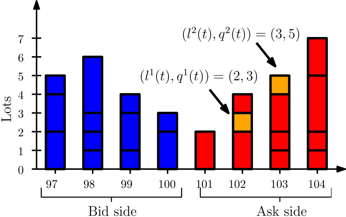
Figure 1 illustrates the state space. The best bid and ask are and The volumes on the bid and ask side are and The algorithm has lots placed in the order book. The first lot has level and queue position and the second lot has level and queue position
3.2 Action space
The algorithm observes states at the discrete time steps right before taking an action For the action space is the simplex
An action represents the allocation of orders to limit and market orders. More precisely, is the fraction of the remaining inventory to be sent as a market order, for is the fraction of the remaining inventory to be placed ticks above the best bid price, and is the fraction of the remaining inventory to be held outside of the order book. We always require that such that the algorithm always posts orders within the visible order book levels defined in (1). For illustration, let us assume that the current inventory is and that With this allocation, the algorithm sends one lot as a market order, five lots as a limit order one tick above the best bid price, three lots as a limit order two ticks above the best bid price, and keeps one lot on the side without placing it in the order book. In the event that the vector includes non-integer values, we round the entries to the closest integer sequentially, always assuring that total allocated orders to not exceed To preserve queue positions, the algorithm only cancels orders if necessary to reach the new allocation when reallocating orders, while prioritizing canceling orders with higher queue positions first.
3.3 Rewards
In each time step the algorithm places market and limit orders according to an action The market orders are filled immediately after leading to an instant cash flow, while the limit orders remain in the book waiting to be filled. The total cash flow from market and limit order fills in the interval is denoted by If any inventory is left at time the algorithm is forced to send a market order of size In that case, the cash flow also contains the proceeds generated by the market order sent at time Suppose that the algorithm sells lots in the interval Then, we define a normalized reward function, which compares the reward to the cash flow that would have been generated by trading at the initial bid price. More precisely, we define
Then objective (2) becomes
| (3) |
which describes the average revenue per lot relative to the initial bid price. The metric in (3) is a normalized version of the industry-standard measure used to evaluate execution algorithms, commonly known as implementation shortfall. We observed in our numerical experiments that normalizing the cash flows increases the training speed of the reinforcement learning algorithm.
Remark 3.1.
Rather than forcing the algorithm to sell any leftover inventory, one could also introduce a soft constraint by using a penalty for the leftover inventory. However, forcing liquidation at terminal time is common in academic papers (Almgren and Chriss, 2001; Nevmyvaka et al., 2006) and is also a reasonable assumption for real-world applications. It is fairly common for traders to set a terminal time at which a trade execution algorithm must complete. For example, depending on the size of the initial inventory, a trader might set the time limit for full liquidation to 10 minutes or the end of the trading day.
3.4 Benchmark algorithms
We compare our trained reinforcement learning algorithm with two heuristic benchmarks and an alternative reinforcement learning algorithm using Dirichlet distributions. The Dirichlet-RL algorithm is explained in Appendix C. The heuristic strategies trade according to the following rules:
-
•
Submit and leave algorithm (SL algorithm): Submits the entire position at as a limit order at the best ask price.
-
•
Time-weighed average price444This is abbreviated with TWAP and represents a standard execution algorithm banks and hedge funds use. algorithm (TWAP algorithm): Divides the position into blocks of size For it posts a limit sell order of size at the best ask price every time step
Both algorithms sell any leftover inventory with a market order.
4 Actor-critic policy gradient with logistic-normal distribution
4.1 Actor-critic policy gradient
The trade execution problem described in Section 3 is a stochastic control problem. The transition probabilities from state to and the reward function are not available in closed form, but we can simulate them. Therefore, the problem can be solved with reinforcement learning. Actor-critic policy gradient algorithms are a class of reinforcement learning algorithms that aim to find an optimal stochastic policy referred to as actor, by estimating the gradient of the objective function A separate parameterized value or advantage function, referred to as critic, is used to reduce the variance of the gradient estimate. We use a neural network with weights to map states to the parameters of the policy’s density. The gradient of the objective function can be computed as
| (4) |
by the policy gradient theorem; see e.g. Schulman et al. (2015). We note that the actions are sampled from a conditional distribution with density and the states are sampled from the market environment. Here, is the advantage function, which is defined as
| (5) |
where is a state and an action at time step
4.2 Policy gradient with logistic-normal distribution
In most applications of policy gradients with continuous action spaces, the multivariate normal distribution is used as an action distribution. However, in our application, the actions must be contained in the simplex. Therefore, we require a distribution with support on the simplex. The works Tian et al. (2022) and Winkel et al. (2023) have used the Dirichlet distribution to achieve this. But we found that the Dirichlet distribution performs sub-optimally in our experiments, even with extensive hyperparameter tuning. An alternative to the Dirichlet distribution is the logistic-normal distribution, which is also defined on the simplex.
The logistic transformation is a function that maps vectors in to actions in where
The inverse mapping is given by
Let be a random variable with multivariate normal distribution on with mean and covariance matrix Then, the transformed random variable has a logistic-normal distribution. The distribution has support and its density function is given by
| (6) |
see, e.g. Atchison and Shen (1980) for a detailed overview of the logistic-normal distribution.
We choose a policy that has logistic-normal distribution with density for each state The parameters are the weights of a neural network (or any other parametric family of functions) that maps states to the mean of the underlying normal distribution We could also make the algorithm learn the covariance matrix But here, we only learn and model as where is the -dimensional identity matrix and a constant that is reduced after each training epoch This allows for exploration at the beginning of training but forces the algorithm to gradually reduce the variance of the stochastic policy until it becomes almost deterministic. Let be the density of the underlying normal distribution on with mean and covariance matrix Since the normalizing constant in (6) does not depend on we obtain for a state and action that
| (7) |
Combining equations (4) and (7) yields
| (8) | ||||
| (9) |
Here means that each element in the sequence is sampled from a normal distribution with conditional density for each state in the sequence We emphasize that the gradient in (9) only affects the density of the underlying normal distribution. The elements are then transformed with to obtain actions without affecting the gradient.
Remark 4.1.
Instead of using the multivariate logistic-normal distribution, one could combine the multivariate normal distribution with a softmax activation function. More precisely, if is a multivariate normal distribution on we could parametrize the policy as , where maps from to with
However, is not bijective. Therefore, it is not possible to derive the policy gradient in closed form as in (9).
4.3 Initialization and scaling of policy parameters
The initialization of the mean and the scaling of the variances of the stochastic policy is an important aspect of training the policy. The mean and covariance of the logistic-normal distribution are not known in closed form. However, for the log ratios, we have
| (10) | ||||
| (11) |
for with the convention and We set the parameters of the last layer of the neural network corresponding to the policy to zero at initialization with a bias term Then, the bias controls the initial allocations of the policy. Furthermore, we choose a diagonal covariance matrix to ensure that unrelated log ratios are uncorrelated. Indeed, for different and equation (11) implies
For indices and with we obtain for the variances of the log ratios that
The initial parameters of the covariance matrix control the initial exploration rate of the policy. As training progresses, we gradually lower the entries in the covariance matrix to discourage exploration and encourage exploitation. For gradient steps and for an initial variance and final variance we set the variances on the diagonal at each gradient step to
| (12) |
The choice of the initial and final variances depends on the application.
4.4 Empirical policy gradient and advantage function estimation
In practice, the expectation (9) is not available, and we replace it with a sample-based estimate. This also requires an estimate of the advantage function (5). We estimate it using an estimate of the value function where are the weights of a neural network. We make gradient steps with respect to the policy parameters and the parameters corresponding to the value function. At the beginning of the training cycle, the parameters are initialized as and In each training epoch we collect trajectories
| (13) |
where the actions are generated by sampling from the underlying normal distribution with density and transformed with For each state action pair the advantage function is estimated as
| (14) |
The parameters of the policy neural network are updated, from to by making a gradient step with learning rate using the loss function
| (15) |
The parameters of the value function neural network are updated, from to by making a gradient step with learning rate using the loss function
| (16) |
Algorithm 1 summarizes the whole training process.
Remark 4.2.
Schulman et al. (2015) describe a general method for estimating advantage functions that interpolates between high-variance/low-bias estimates and low-variance/high-bias estimates. Estimate (14) has low bias but high variance. We reduce the variance of the estimate by using a large number of trajectories at each gradient step.
5 Market environment
We test our RL algorithm in a market environment populated by three different types of traders: noise traders who place and cancel orders randomly, tactical traders who react to order book imbalance, and a strategic trader who buys or liquidates a large position with a TWAP strategy, and therefore, trades in one direction at constant speed. We simulate the order book in the interval
5.1 Noise traders
Our first category of traders are noise traders who submit market, limit, and cancellation orders according to independent Poisson processes (Cont et al., 2010; Abergel and Jedidi, 2013). The intensities of market orders, limit orders, and cancellations arrivals are modeled in the following way.
-
•
Market buy and sell orders arrive with intensity
-
•
For limit buy and sell orders arrive with intensity at ticks below the best ask price and ticks above the best bid price, respectively.
-
•
If the spread is ticks, then for cancellations of limit buy orders arrive with intensity at ticks below the best ask price, and cancellations of limit sell orders arrive with intensity at ticks above the best bid price.
5.2 Tactical traders
In contrast to the noise traders, the intensities of the tactical traders depend on volume imbalance. We define weighted volumes on the bid and ask sides by
where is a damping factor. The weighted volume imbalance is then defined by
The damping factor effectively controls how sensitive the imbalance is to volumes posted at deeper levels in the book. Let and be the positive and negative parts of the imbalance. The intensities for different order types are defined as follows.
-
•
For market buy orders arrive with intensity and market sell orders arrive with intensity
-
•
For limit buy orders arrive with intensity at ticks below the best ask price, and limit sell orders with intensity at ticks above the best bid price.
-
•
If the spread is ticks, then for cancellation of limit buy orders arrive with intensity at ticks below the best ask price, and and cancellations of limit sell orders arrive with intensity at ticks above the best bid price.
For market orders, limit orders and cancellations arrive with sizes and respectively, where is a random variable with a standard normal distribution for both noise and tactical traders. Order sizes are always rounded to the closest integer. Furthermore, both types of traders always cancel orders with the highest queue positions first, and no more orders can be canceled than exist at a given level.
5.3 Strategic traders
The strategic trader buys or sells a position in the market using limit and market orders.
-
•
The direction, either buy or sell, is drawn randomly at the start time with probability each.
-
•
The trader sends a market order of size at time steps and stops trading at terminal time
-
•
The trader sends a limit order of size at time steps and stops trading at terminal time
6 Numerical results
In this section, we test our RL-algorithm based on the logistic-normal distribution (LN) in different simulated market environments and compare it with the two heuristic benchmarks from Section 3.4 and another RL-algorithm based on the Dirichlet distribution (DR), explained in Appendix C below. Our source code is available at https://github.com/moritzweiss/rlte.
6.1 Simulation setup
We simulate three increasingly complex market environments. The first market contains only noise traders and serves as a baseline. Price movements are entirely random, with no response from market participants. The second market includes both noise traders and tactical traders. In this setting, order flows react to order book imbalances, a behavior commonly observed in empirical studies of limit order book dynamics; see e.g. Stoikov (2018). The third market adds a strategic trader to the previous participants. It simulates a market that exhibits upward or downward price drift due to the presence of a strategic trader. This drift requires the execution algorithm to adapt its execution strategy by front-loading or back-loading orders. While such pronounced trends are rare in real markets, this environment tests whether the algorithm can detect directional signals from order book features and adjust its behavior accordingly. Although these simulations are stylized, they capture key characteristics of real-world market behavior. Importantly, our simulations differ significantly from historical market data replay because in our simulations, trades generate market impact. First, large market orders have direct impact since they consume the best levels on the opposite side of the order book. Second, limit orders have indirect impact as the tactical traders react to order book imbalance. Those effects cannot be incorporated in a simulation relying on historical data replay, as the data is fixed and does not react to the algorithm’s trading decisions. We compare both algorithms with the heuristic algorithms555We refer to the LN and DR algorithms and the benchmark algorithms as execution algorithms. defined in Section 3.4, in each of the three market environments, and for small and large positions to be liquidated.
As mentioned in Section 3, the execution algorithms trade at discrete time steps for For our simulations, we choose for a total of steps, such that the total execution duration is We use a short simulation horizon to reduce computational overhead during training. This choice does not compromise the validity of our results, as the underlying logic and outcomes would also hold for longer execution horizons. In each market, the execution algorithms trade a small (20) and a large (60) number of lots. What can be considered a small or large number of lots depends on the average traded volume in the interval In our examples, the average traded volume over the time interval is 100 lots in each market. When adding a new trader to the market, we adjust the trading intensities of the other traders so that the overall average trading volume remains the same at 100 lots. Hence, 20 lots correspond to 20% and 60 lots correspond to 60% of the total traded volume. In all three markets, we start the simulation at time where at initialization, we set the order book to its long-term average shape. Therefore, when the execution algorithms start trading at the order book has moved from its initial state to a random state. The average shape of the order book can be estimated with a Monte Carlo simulation, which is described in more detail in Appendix A.2. The specific parameter choices for each trading agent are discussed in Appendix A.1.
We use the two heuristic strategies of Section 3.4 as benchmarks and introduce an additional benchmark based on the Dirichlet distribution, which is explained in more Detail in Section C. It would also be feasible to compare against other trade execution benchmark algorithms, such as the volume-weighted-average price algorithm. However, our algorithm is not directly comparable with other reinforcement learning algorithms that have been mentioned in the introduction. This has two reasons. First, algorithms developed on simulations relying on historical data are not comparable because our market simulation is inherently different from historical market data replay. Second, none of the related research works use the same state and action spaces formulation. In particular, no other work views the order placement problem as a dynamic allocation problem.
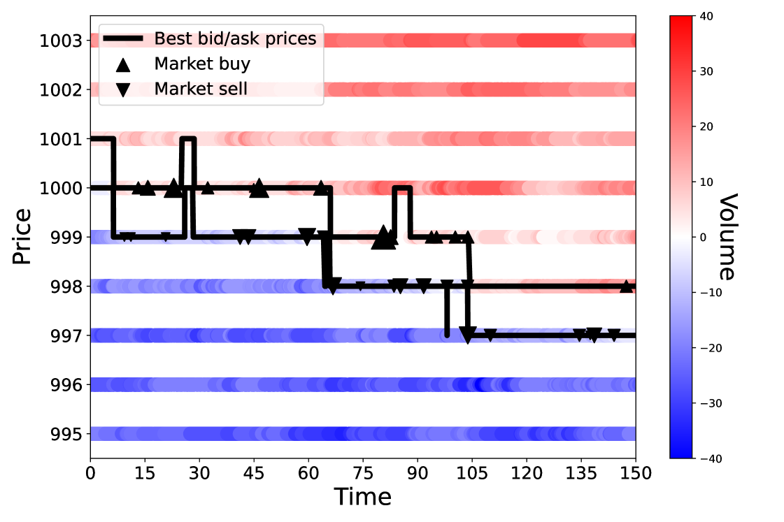
Figure 2 shows an evolution of the order book in the interval for the market with only noise traders. The bid and ask prices move from and three ticks down to and The composition of the order book changes due to the arrival of market orders, limit orders, and cancellations.
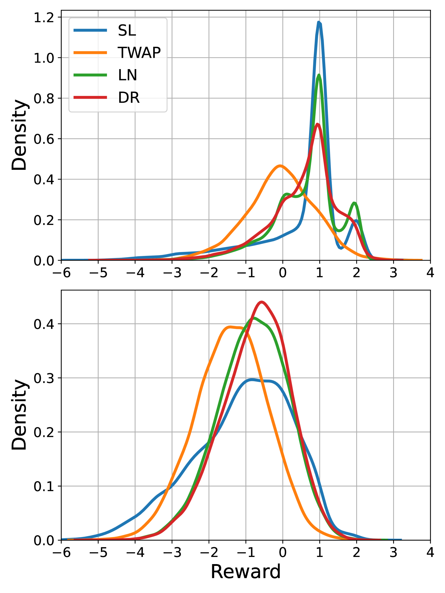
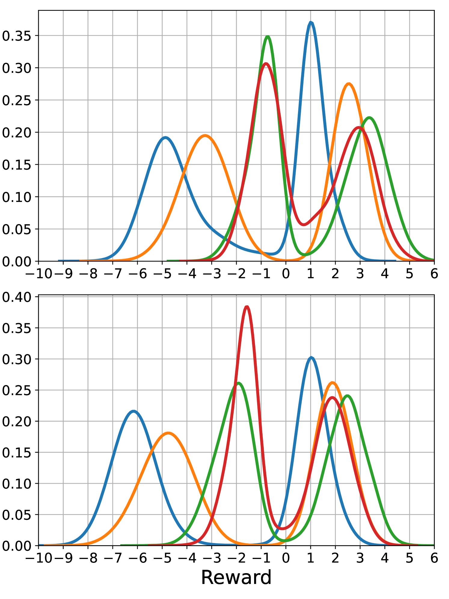
The test results are summarized in Table 1, which contains the expected value and the standard deviation of the sum of normalized rewards defined in (3) for all market environments, position sizes, and execution algorithms. For example, the reward of for the SL algorithm at 60 lots in the market with noise traders means that on average, the algorithm sold each of the 60 lots at ticks less than the initial bid price. The plots in Figure 3 show histograms of normalized rewards based on 10,000 simulated executions. The random seeds used for the processes of different trading agents are selected independently from those employed during training, thereby avoiding over-fitting to the training simulations.
6.2 Reinforcement learning setup
We train the LN algorithm with Algorithm 1. As explained in Sections 3.1–3.2, the parameter controls how many order book levels the algorithm observes and how deep it may post orders into the order book. In our simulations, the price rarely moves more than five ticks throughout the execution horizon. Therefore, we choose for the dimension of the simplex This means that the RL algorithm may place limit orders up to five ticks above the best bid price and observes the volumes on the first five levels on both sides of the book. To encode the policy and the value function we choose two separate feed-forward neural networks with two hidden layers, -activation functions in the hidden layers and no activation functions in the last layers. The output layer of the policy network has nodes, and the last layer of the value function network has one node. We start by setting the covariance matrix to the identity matrix and then progressively reduce its values according to the linear schedule (12). We choose an initial bias for the policy network. We obtain from (10) that
showing that action is more likely than actions This means the algorithm does not place any orders at the start of the training cycle, which ensures that the algorithm observes complete trajectories up to the terminal time early in the training process, preventing it from getting stuck in local minima. Further implementation details concerning the training of the LN algorithm are discussed in Appendix B.
6.3 Logistic-normal vs Dirichlet distribution
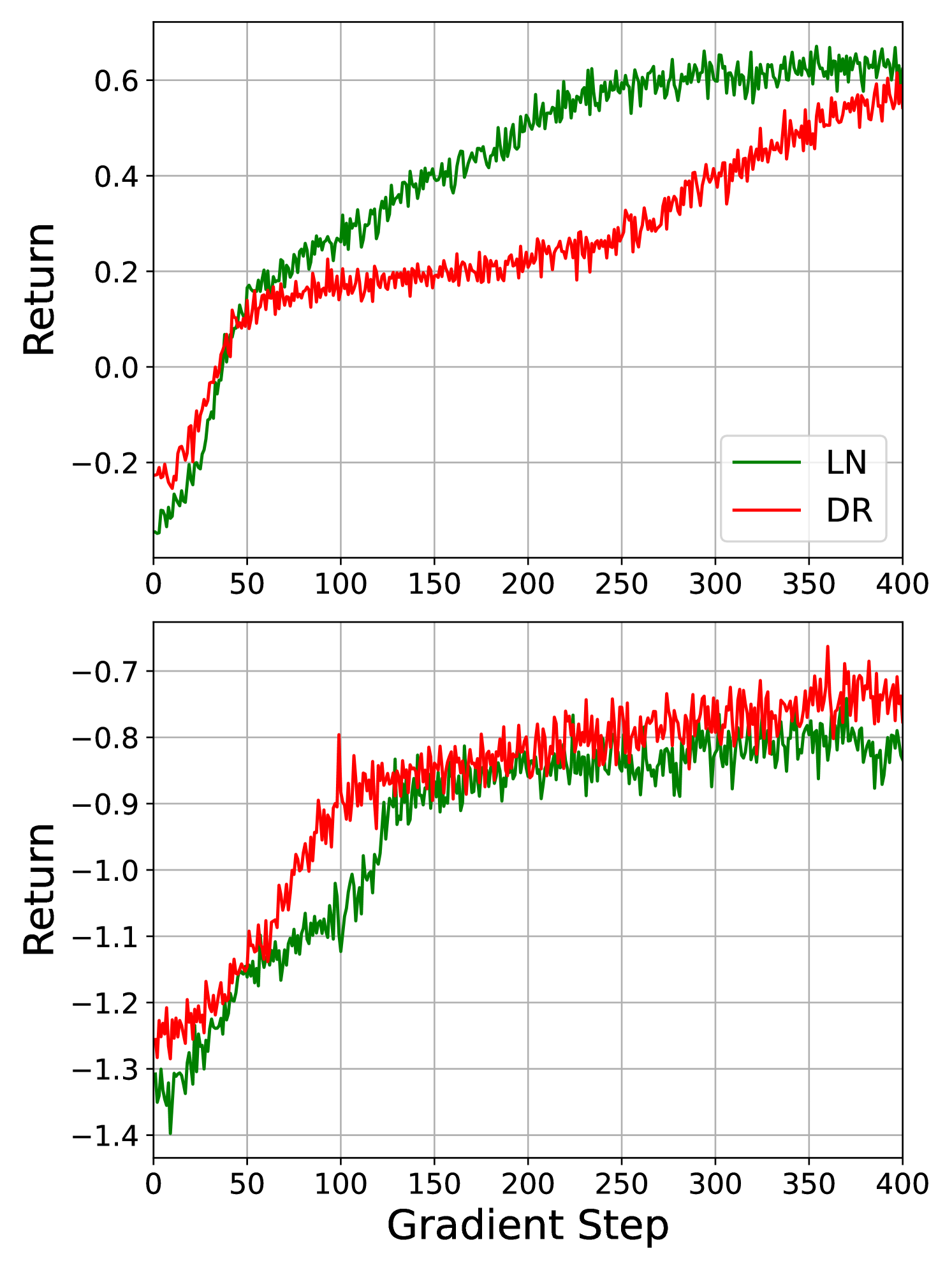
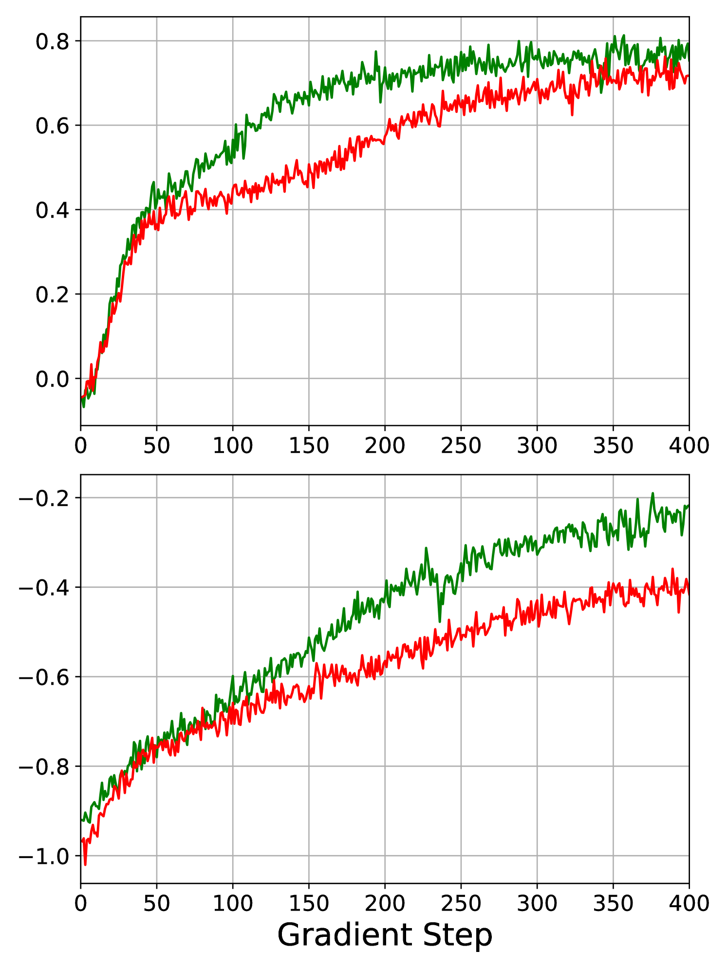
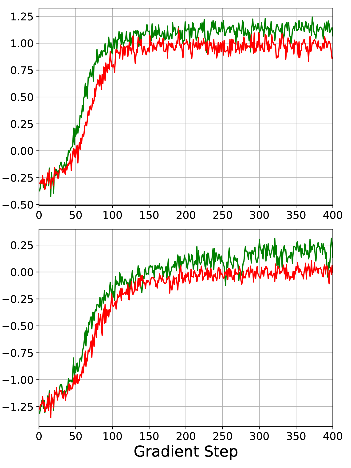
First of all, we observe that in all three market simulations, the LN algorithm outperforms the DR algorithm, which is visible in Table 1 and Figure 3. Figure 4 shows the development of the episode returns over the full training cycle. The upper panel shows the results for 20 lots, and the lower panel shows the results for 60 lots. We observe that in all experiments, except when the agent executes 20 lots in the market only containing noise traders, the rewards for the LN algorithm converge faster than for the DR algorithm. This suggests that the LN algorithm is a superior alternative to the DR algorithm in this allocation problem. As the performance of the LN and DR algorithms is qualitatively similar, we focus our attention on the performance of the LN algorithm relative the the heuristic benchmarks in the following sections.
| Market | #Lots | ||||||||
|---|---|---|---|---|---|---|---|---|---|
| Noise | 20 | 0.52 | 1.20 | -0.05 | 0.94 | 0.58 | 0.90 | 0.65 | 0.89 |
| 60 | -1.10 | 1.34 | -1.40 | 0.97 | -0.74 | 0.92 | -0.69 | 0.91 | |
| Noise & Tactical | 20 | 0.10 | 1.43 | 0.48 | 0.68 | 0.73 | 0.67 | 0.79 | 0.69 |
| 60 | -3.36 | 0.99 | -0.96 | 0.95 | -0.41 | 0.63 | -0.25 | 0.65 | |
| Noise & Tactical | 20 | -1.61 | 2.95 | -0.31 | 3.03 | 0.86 | 1.92 | 1.16 | 2.08 |
| & Strategic | 60 | -2.46 | 3.67 | -1.40 | 3.46 | -0.02 | 1.90 | 0.16 | 2.04 |
6.4 Market with noise traders
The first two rows of Table 1 demonstrate that the LN algorithm outperforms both heuristic benchmarks and the DR algorithm for 20 and 60 lots. This is also visible in the histograms in Figure 3(a). We remark that all algorithms in all markets have a high standard deviation. This is unavoidable as the algorithms operate in a highly stochastic environment. Sending a market order at the beginning of the execution period would result in a strategy with almost zero standard deviation; however, the execution price would be worse than the initial best bid and, therefore, worse than most of our execution strategies. For 20 lots, the LN algorithm’s histogram plot exhibits a bump at one and two ticks above the best bid price, indicating that it places limit orders deeper in the book and cuts losses when the price moves against it. For 60 lots, while the histograms of the LN and SL algorithms appear similar, the LN algorithm’s histogram exhibits less skew to the left, further suggesting that it effectively limits losses when the market moves away. The TWAP algorithm has the worst performance for both position sizes. Since the market does not react to volume imbalance, placing the entire position passively at the start has no downside.
6.5 Market with noise & tactical traders
The third and fourth rows of Table 1 and Figure 3(b) display the results for the market consisting of noise and tactical traders. Both demonstrate the LN algorithm’s superior performance relative to the benchmark algorithms for small and large position sizes. The performance of the LN algorithm is slightly better than the DR algorithm. As before, for 20 lots, we observe bumps in the histogram at one and two ticks above the best bid price for the LN algorithm. For lots, the LN algorithm’s histogram has less left skew than the benchmark densities, indicating that it cuts losses when prices move against it. The presence of tactical traders reacting to order book imbalances introduces indirect market impact. Consequently, posting the entire position passively at the beginning, as done by the SL algorithm, triggers the tactical traders to trade in the other direction, leading to the worst performance. Spreading the order out over the whole time horizon, as done by the TWAP algorithm, is better. Still, the LN algorithm performs best, suggesting intelligent placement strategies.
6.6 Market with noise & tactical & strategic traders
The fifth and sixth rows of Table 1 and Figure 3(c) show the results for the market consisting of noise, tactical, and strategic traders and demonstrate the strong performance of the LN algorithm. The presence of a strategic trader introduces an upward or downward drift in the market. The LN algorithm detects this drift using the historical market and limit order flow features and the mid-price drift feature defined in Section 3.1. The performance of the LN algorithm is slightly better than the DR algorithm. The relative shift of the LN algorithm’s histogram compared to those of the benchmark algorithms suggests that it trades more aggressively when the strategic trader is selling and more patiently when the strategic trader is buying.
7 Conclusion
We have developed an execution algorithm based on a novel actor-critic policy gradient approach that uses the logistic-normal distribution to model random allocations. Its state space captures all relevant market features, including current and past states of the order book and queue positions. The action space allows the algorithm to place market and limit orders across multiple price levels, adapting to changing market conditions. The algorithm outperforms competitive benchmarks in realistic simulations that account for direct and indirect market impact. This is the first time the logistic-normal distribution has been combined with the actor-critic algorithm. Our results suggest that this is a better approach than using the Dirichlet distribution since our algorithm shows better results and faster convergence speeds.
The strength of our results is inherently tied to the realism of the market simulation. While our simulations capture key stylized facts of limit order book markets, they do not fully replicate real-world conditions. Nevertheless, our method remains broadly applicable and can be used with any market simulation framework and institutional investors may combine our method with their own proprietary market simulations.
References
- Abergel and Jedidi (2013) Frédéric Abergel and Aymen Jedidi. A mathematical approach to order book modeling. International Journal of Theoretical and Applied Finance, 16(05):1350025, 2013.
- Almgren (2003) Robert Almgren. Optimal execution with nonlinear impact functions and trading-enhanced risk. Applied Mathematical Finance, 10(1):1–18, 2003.
- Almgren (2012) Robert Almgren. Optimal trading with stochastic liquidity and volatility. SIAM Journal on Financial Mathematics, 3(1):163–181, 2012.
- Almgren and Chriss (2001) Robert Almgren and Neil Chriss. Optimal execution of portfolio transactions. Journal of Risk, 3:5–40, 2001.
- Atchison and Shen (1980) Jhon Atchison and Sheng M Shen. Logistic-normal distributions: Some properties and uses. Biometrika, 67(2):261–272, 1980.
- Bertsimas and Lo (1998) Dimitris Bertsimas and Andrew W. Lo. Optimal control of execution costs. Journal of Financial Markets, 1(1):1–50, 1998.
- Bouchaud et al. (2018) Jean-Philippe Bouchaud, Julius Bonart, Jonathan Donier, and Martin Gould. Trades, Quotes and Prices: Financial Markets Under the Microscope. Cambridge University Press, 2018.
- Byrd et al. (2020) David Byrd, Maria Hybinette, and Tucker Hybinette Balch. Abides: Towards high-fidelity multi-agent market simulation. In Proceedings of the 2020 ACM SIGSIM Conference on Principles of Advanced Discrete Simulation, pages 11–22, 2020.
- Byun et al. (2023) Woo Jae Byun, Bumkyu Choi, Seongmin Kim, and Joohyun Jo. Practical application of deep reinforcement learning to optimal trade execution. FinTech, 2(3):414–429, 2023.
- Cartea and Jaimungal (2015) Alvaro Cartea and Sebastian Jaimungal. Optimal execution with limit and market orders. Quantitative Finance, 15(8):1279–1291, 2015.
- Cartea and Jaimungal (2016) Álvaro Cartea and Sebastian Jaimungal. Incorporating order-flow into optimal execution. Mathematics and Financial Economics, 10:339–364, 2016.
- Cheridito and Sepin (2014) Patrick Cheridito and Tardu Sepin. Optimal trade execution under stochastic volatility and liquidity. Applied Mathematical Finance, 21(4):342–362, 2014.
- Cont et al. (2010) Rama Cont, Sasha Stoikov, and Rishi Talreja. A stochastic model for order book dynamics. Operations Research, 58(3):549–563, 2010.
- Curato et al. (2017) Gianbiagio Curato, Jim Gatheral, and Fabrizio Lillo. Optimal execution with non-linear transient market impact. Quantitative Finance, 17(1):41–54, 2017.
- Di Giacinto et al. (2024) Marina Di Giacinto, Claudio Tebaldi, and Tai-Ho Wang. Optimal order execution under price impact: a hybrid model. Annals of Operations Research, 336(1):605–636, 2024.
- Gatheral and Schied (2011) Jim Gatheral and Alexander Schied. Optimal trade execution under Geometric Brownian Motion in the Almgren and Chriss framework. International Journal of Theoretical and Applied Finance, 14(03):353–368, 2011.
- Gatheral and Schied (2013) Jim Gatheral and Alexander Schied. Dynamical models of market impact and algorithms for order execution. Handbook on Systemic Risk, Jean-Pierre Fouque, Joseph A. Langsam, eds, pages 579–599, 2013.
- Gould et al. (2013) Martin D Gould, Mason A Porter, Stacy Williams, Mark McDonald, Daniel J Fenn, and Sam D Howison. Limit order books. Quantitative Finance, 13(11):1709–1742, 2013.
- Guéant and Lehalle (2015) Olivier Guéant and Charles-Albert Lehalle. General intensity shapes in optimal liquidation. Mathematical Finance, 25(3):457–495, 2015.
- Hafsi and Vittori (2024) Yadh Hafsi and Edoardo Vittori. Optimal execution with reinforcement learning. arXiv Preprint arXiv:2411.06389, 2024.
- Hendricks and Wilcox (2014) Dieter Hendricks and Diane Wilcox. A reinforcement learning extension to the Almgren–Chriss framework for optimal trade execution. In 2014 IEEE Conference on Computational Intelligence for Financial Engineering & Economics, pages 457–464, 2014.
- Huang et al. (2022) Shengyi Huang, Rousslan Fernand Julien Dossa, Chang Ye, Jeff Braga, Dipam Chakraborty, Kinal Mehta, and João G. M. Araújo. Cleanrl: High-quality single-file implementations of deep reinforcement learning algorithms. Journal of Machine Learning Research, 23(274):1–18, 2022.
- Kingma and Ba (2017) Diederik P Kingma and Jimmy Lei Ba. Adam: A method for stochastic optimization. arXiv Preprint arXiv:1412.6980, 2017.
- Leal et al. (2022) Laura Leal, Mathieu Laurière, and Charles-Albert Lehalle. Learning a functional control for high-frequency finance. Quantitative Finance, 22(11):1973–1987, 2022.
- Moallemi and Wang (2022) Ciamac C Moallemi and Muye Wang. A reinforcement learning approach to optimal execution. Quantitative Finance, 22(6):1051–1069, 2022.
- Nevmyvaka et al. (2006) Yuriy Nevmyvaka, Yi Feng, and Michael Kearns. Reinforcement learning for optimized trade execution. In Proceedings of the 23rd international conference on Machine learning, pages 673–680, 2006.
- Ning et al. (2021) Brian Ning, Franco Ho Ting Lin, and Sebastian Jaimungal. Double deep Q-learning for optimal execution. Applied Mathematical Finance, 28(4):361–380, 2021.
- Obizhaeva and Wang (2013) Anna A Obizhaeva and Jiang Wang. Optimal trading strategy and supply/demand dynamics. Journal of Financial markets, 16(1):1–32, 2013.
- Saxe et al. (2013) Andrew M Saxe, James L McClelland, and Surya Ganguli. Exact solutions to the nonlinear dynamics of learning in deep linear neural networks. arXiv Preprint arXiv:1312.6120, 2013.
- Schulman et al. (2015) John Schulman, Philipp Moritz, Sergey Levine, Michael Jordan, and Pieter Abbeel. High-dimensional continuous control using generalized advantage estimation. arXiv Preprint arXiv:1506.02438, 2015.
- Stoikov (2018) Sasha Stoikov. The micro-price: a high-frequency estimator of future prices. Quantitative Finance, 18(12):1959–1966, 2018.
- Tian et al. (2022) Yuan Tian, Minghao Han, Chetan Kulkarni, and Olga Fink. A prescriptive Dirichlet power allocation policy with deep reinforcement learning. Reliability Engineering & System Safety, 224:108529, 2022.
- Winkel et al. (2023) David Winkel, Niklas Strauß, Matthias Schubert, and Thomas Seidl. Simplex decomposition for portfolio allocation constraints in reinforcement learning. In ECAI, pages 2655–2662. IOS Press, 2023.
Appendix A Parameters and stationary order book shapes in the market simulation
A.1 Parameters for market simulations
We assume that the noise and tactical traders submit orders (market orders, limit orders and cancellations) up to level and that all of their orders have the same shifted half-normal distribution with parameters for We cap large order sizes at five standard deviations because very large order sizes are unrealistic. We always start the simulations at from an equilibrium state and run them until time The equilibrium states are explained in more detail in Appendix A.2 below. The LN-RL, DR-RL, and all benchmark algorithms trade during the time interval [0, T], updating their decisions at the times for and The parameters are summarized in Table 2.
| start time for noise, tactical & strategic traders | |
| initial bid price | 1000 |
| initial ask price | 1001 |
| end time | |
| 10 | |
| 2 | |
| see table below | |
| 2 | |
| 1 | |
| 2 | |
| probability Buy or sell strategic trader | |
| start time for RL and benchmark algorithms | |
| small initial position | 20 |
| large initial position | 60 |
Market with noise traders
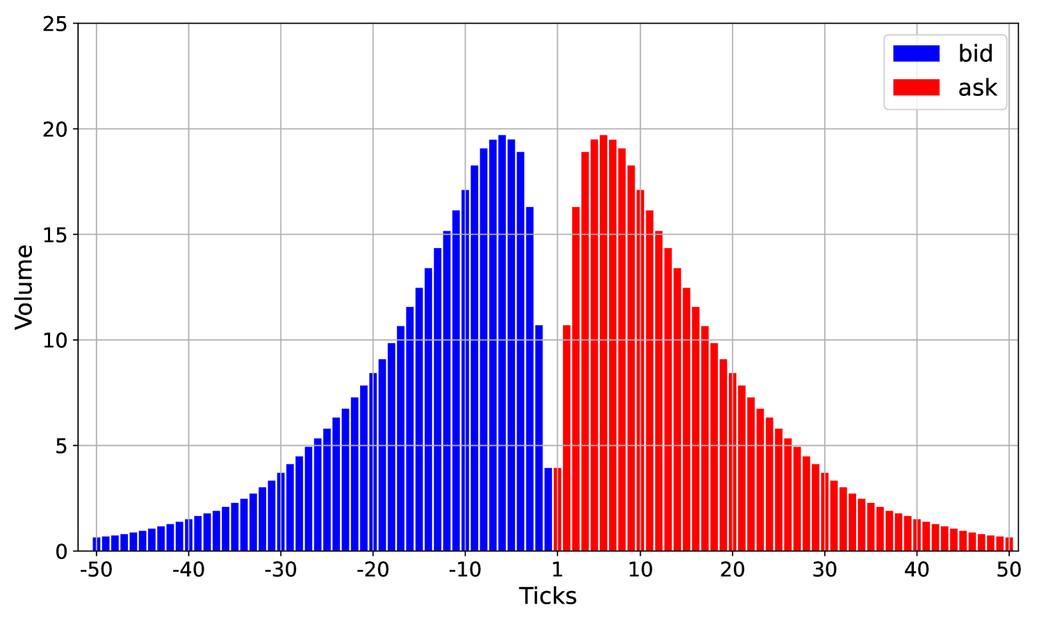
The intensities of limit order arrivals and cancellations for the noise traders are given in Table 3. The market order intensity is Those intensities are taken from the paper Abergel and Jedidi (2013) with one modification. Instead of the cancellation intensities in that paper, we increase the cancellation intensities by a factor of This leads to smaller queue sizes, which makes the simulation more efficient. At , we set the limit order book equal to its equilibrium shape. It is displayed in Figure 5(a). The average total traded volume in this market is 100 lots.
| (ticks) | ||
|---|---|---|
| 1 | 0.2842 | 0.8636 |
| 2 | 0.5255 | 0.4635 |
| 3 | 0.2971 | 0.1487 |
| 4 | 0.2307 | 0.1096 |
| 5 | 0.0826 | 0.0402 |
| 6 | 0.0682 | 0.0341 |
| 7 | 0.0631 | 0.0311 |
| 8 | 0.0481 | 0.0237 |
| 9 | 0.0462 | 0.0233 |
| 10 | 0.0321 | 0.0178 |
| 11 | 0.0178 | 0.0127 |
| 12 | 0.0015 | 0.0012 |
| 13 | 0.0001 | 0.0001 |
| 14 | 0.0000 | 0.0000 |
| ⋮ | ⋮ | ⋮ |
| 30 | 0.0000 | 0.0000 |
Market with noise & tactical traders
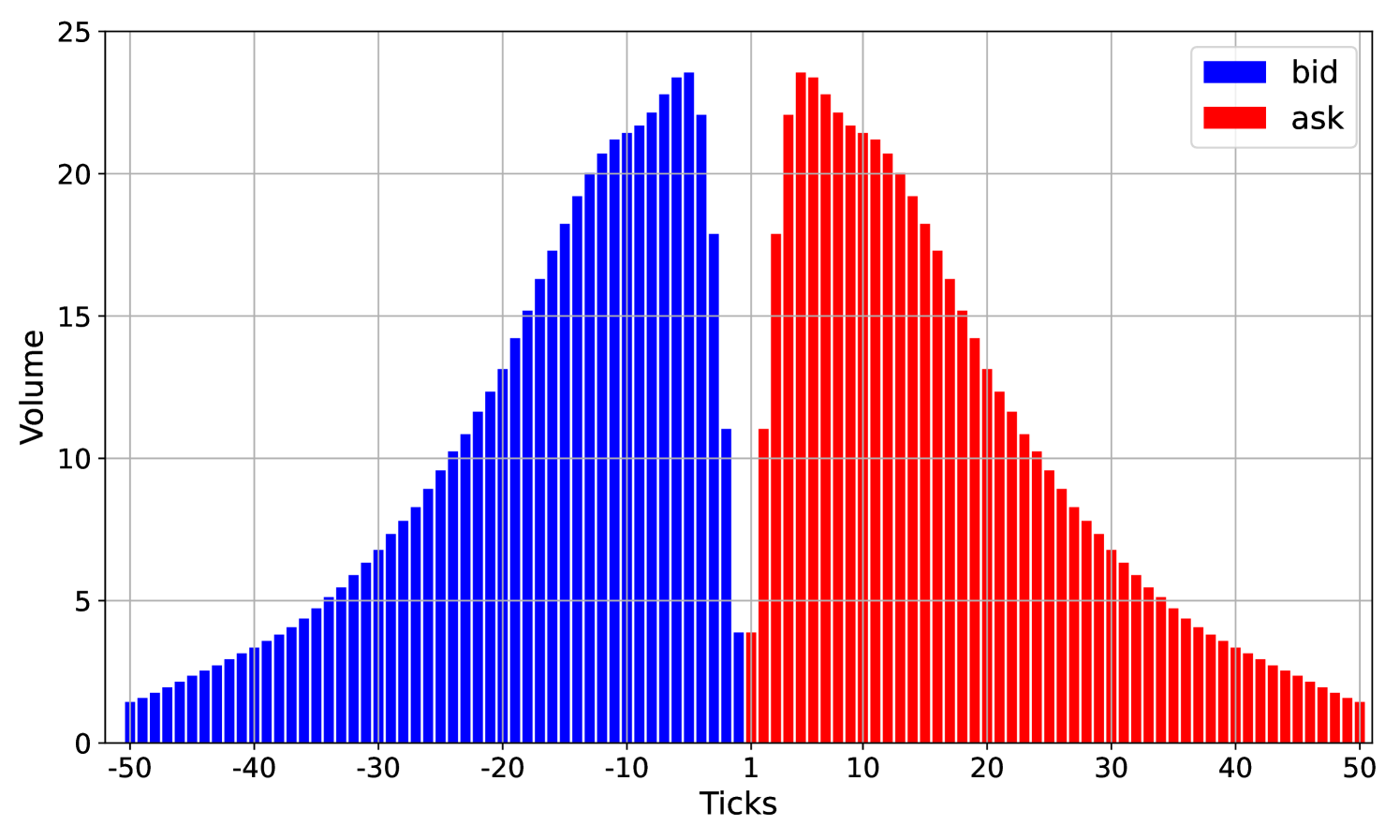
For the tactical traders, we choose a damping factor and constant imbalance reaction factors for To compensate for the presence of tactical traders, we reduce the intensities of the noise traders by 15%. With this intensity reduction, the average total traded volume over the trading horizon is roughly the same for the market with noise traders only and the market with noise and tactical traders. We start the simulation at from its equilibrium state, displayed in Figure 5(b).
Market with noise & tactical & strategic traders
We combine noise, tactical, and strategic traders for the third market. The parameters for noise and tactical traders remain the same as in the previous market simulations, except that we reduce the intensities of the noise and tactical traders by 10% to account for the presence of the strategic trader. This way, the total average traded volume is roughly the same for all market environments. The strategic trader sends a limit order of size every seconds and a market order of size every seconds. Due to the presence of the strategic trader, this market does not have an equilibrium state. At time we start the order book from the same shape as in the market with noise and tactical traders. The trade direction of the strategic trader (buying or selling) is drawn randomly with probability at the time
Small and large initial positions
The total average traded volume in all three simulated markets is roughly the same. Therefore, the results for the initial positions of 20 and 60 lots in Table 1 are comparable across all markets, as in all markets this accounts for roughly 20% and 60% of the total volume.
A.2 Stationary order book shapes
We always start the market simulation from an equilibrium state of the limit order book. The equilibrium states are described by the average queue sizes and the average spread:
| (17) |
Here, for the quantity is the average volume ticks below the best bid price and is the average volume ticks above the best ask price. Since the average spread in our simulations is always close to one tick, we start all simulations with an initial bid price and an initial ask price . An asset with an average spread close to one tick is called large tick asset.
We find such an equilibrium state by running the market simulation for a long time and then averaging. This equilibrium state is shown in Figure 5(a) for the first market consisting only of noise traders. For the second market, consisting of noise and a strategic trader, this equilibrium state is shown in Figure 5(b). We observe that the shapes look similar but are not quite the same. In particular, the market with noise and tactical traders has more volume at the best bid and ask prices. The third market, consisting of noise traders, tactical traders, and a strategic trader, does not have an equilibrium state due to the presence of the strategic trader.
Appendix B Hyperparameters and implementation details for the actor-critic algorithm
We implemented an actor-critic reinforcement learning algorithm that solves a dynamic allocation problem using the logistic-normal distribution. Our implementation is based on the implementation of the proximal policy optimization algorithm (PPO) by Huang et al. (2022); see https://github.com/vwxyzjn/cleanrl. We implemented the following changes. First, we are not using clipping. Second, we implemented a custom logistic-normal action policy. Third, we implemented the custom initialization of the mean and covariance matrix and the scaling of the covariance matrix during the training loop described in Section 4.3.
In this section, we provide a detailed description of the algorithm’s hyperparameters. They are summarized in Table 4 and Table 5.
| Number of parallel environments | |
| Steps per environment | |
| Number of Trajectories | 1,280 |
| Length of Trajectories | |
| Training Iterations H | 400 |
| Learning Rate | |
| Linear Variance scaling | True |
| Initial variance | 1 |
| Final variance | 0.1 |
| Simplex Dimension | 6 |
| Number of hidden layers | |
| Nodes of in hidden layers | |
| Nodes of output layer for value function network | |
| Nodes of output layer for policy function network | |
| Activation functions for hidden layers | |
| Activation functions for last layers | None |
Neural network architecture
For the value function and the policy we use two separate neural networks with two hidden layers with nodes. The hidden layers have a activation function and the last layers have no activation function. The last layer of the policy network has nodes corresponding to the mean vector of the normal distribution with density The last layer of the value function network has one node. We initialize the weights of both neural networks with an orthogonal initialization scheme; see e.g. Saxe et al. (2013). For the last layer of the policy network, we set the bias to and initialize the weights using orthogonal initialization with a gain factor Therefore, the weights of the last layer of the policy network are close to zero and the output is effectively determined by the bias term. For all other layers in the policy and value function neural networks, we use an orthogonal initialization with a gain factor to initialize the weights and set the bias terms to zero.
Vectorized sample collection
We use a vectorized architecture to collect samples from the market simulation. We use parallel markets, using 128 CPUs, where each market collects 10 trajectories. This results in a total number of trajectories. In each training iteration, we sample a batch of trajectories
| (18) |
Learning phase
We use the Adam optimizer (Kingma and Ba, 2017) with a learning rate (also referred to as step-size) of In all experiments, we make gradient steps. We set the initial covariance matrix of the normal distribution equal to the unit matrix in We choose the initial and final variance and and, in each training iteration reduce the diagonal entries according to the schedule (12).
Appendix C Implementation details for Dirichlet reinforcement learning algorithm
Dirichlet distribution
Let with . The Dirichlet distribution is defined on the probability simplex:
The probability density function is defined by
RL algorithm
As for the logistic-normal distribution, we use the policy gradient theorem (4) to train the algorithm. The parameters of the density are the output of a neural network. To ensure that the parameters are positive, we use the soft-plus function, defined as in the output layer as an activation function. We choose the soft-plus function over the exponential function to prevent the parameters from becoming excessively large, which could lead to a concentrated policy. Furthermore, when initializing the policy neural network, we choose the weights of the output layer close to This ensures that the action has more weight than the other actions. Therefore, at the beginning of the training cycle, the algorithm will not place many orders, observing full trajectories. The neural network architecture for the value function network is the same as above.
Appendix D Feature normalization
The features described in Section 3.1 are normalized in our implementation. We generally aimed to normalize all features to the same scale by transforming them to the interval or We present each feature’s normalized counterpart in the following bullet points.
Market states
-
•
We normalize bid and ask prices around the initial prices. More specifically, we use and In our simulations, the prices rarely move more than five ticks, which justifies our normalization.
-
•
We recall from Section 3.1 that the algorithm observes the first entries of the order book volumes defined in equation (1). Instead of the absolute, we consider the normalized volumes on the bid and ask sides and We normalize the volumes by using the long-term average queue sizes defined in Appendix A.2, as follows:
The average queue sizes are estimated by running the simulation for a long time and computing averages as described in Appendix A.2. For the market consisting of noise traders only, we normalize with the long-term average shape of that market, which is displayed in Figure 5(a). For the market consisting of noise and tactical traders, we normalize with the long-term average shape of that market, which is displayed in Figure 5(b). There is no stable long-term average shape for the market consisting of noise, tactical, and strategic traders as the market drifts up or down. In this case, we normalize the volumes using the average shapes corresponding to the market with noise and tactical traders (Figure 5(b)).
-
•
We normalize the market order flow in by dividing it by the total volume of all market buy and sell orders in . The normalized market order flow is then contained in
-
•
We normalize the limit order flow in by dividing it by the total volume of all limit buy and sell orders in . The normalized limit order flow is then contained in
-
•
We normalize the mid-price drift relative to the previous mid-price by considering
Private states
-
•
We normalize the current time relative to the final time by considering
-
•
We normalize the inventory relative to the initial inventory by considering
-
•
We normalize the number of active limit orders in the book relative to the inventory by considering
-
•
If there are active limit orders in the book, and is the number of lots that are withheld from the order book, and the remaining orders have already been filled, then we encode the levels of all limit orders by
Here, for the quantity is the level of the active limit orders, ordered from the smallest to the highest price levels. For we set where is the dimension of For we set
-
•
If there are active limit orders in the book, and is the number of lots that are outside the book, and the remaining orders have already been filled, then we encode the queue positions of all limit orders by
Here, for the quantity is the queue position of the active limit orders, ordered from the smallest to the highest price levels and queue positions. For we set For we set In our simulations, the queue sizes are rarely larger than (see Figures 5(a) and 5(b)), which justifies the normalization of the queue positions by
-
•
We use one additional feature, representing the number of active orders per price level, given by where is the dimension of the simplex containing the actions. For the quantity is the fraction of the inventory that is placed at ticks above the best ask and is the fraction of the inventory that is either placed higher than ticks away from the best ask price or not placed in the book. We note that the feature is redundant since the algorithm already has information on the levels of its limit orders through the vector However, we noticed that the inclusion of improves the convergence speed of the algorithm.