SMReferences
Reinforcement Learning with Continuous Actions Under Unmeasured Confounding
Abstract
This paper addresses the challenge of offline policy learning in reinforcement learning with continuous action spaces when unmeasured confounders are present. While most existing research focuses on policy evaluation within partially observable Markov decision processes (POMDPs) and assumes discrete action spaces, we advance this field by establishing a novel identification result to enable the nonparametric estimation of policy value for a given target policy under an infinite-horizon framework. Leveraging this identification, we develop a minimax estimator and introduce a policy-gradient-based algorithm to identify the in-class optimal policy that maximizes the estimated policy value. Furthermore, we provide theoretical results regarding the consistency, finite-sample error bound, and regret bound of the resulting optimal policy. Extensive simulations and a real-world application using the German Family Panel data demonstrate the effectiveness of our proposed methodology.
Keywords: Reinforcement Learning, Policy Optimization, Policy Evaluation, Causal Inference, Confounded POMDP
1 Introduction
In practical applications of reinforcement learning (RL) (Sutton and Barto, 2018), the evaluation and optimization of policies using only pre-collected datasets has become essential. This need arises from the potential costs and safety risks associated with frequent interactions with the environment, such as real-world testing in autonomous driving (Zhu et al., 2020) and treatment selection in precision medicine (Luckett et al., 2019; Zhou et al., 2024a). As a result, there has been a growing interest in offline RL (Precup, 2000; Levine et al., 2020), which focuses on policy evaluation and optimization without requiring additional environment interactions.
Recent years have seen significant advancements in both off-policy evaluation (OPE) and off-policy learning (OPL). In OPE, popular methodologies include value-based approaches (Le et al., 2019; Liao et al., 2021), importance sampling techniques (Liu et al., 2018; Xie et al., 2019), and doubly robust methods that integrate value-based and importance sampling estimators (Uehara et al., 2020; Kallus et al., 2022). Additionally, confidence intervals for a target policy have been developed using bootstrapping (Hao et al., 2021), asymptotic properties (Shi et al., 2022b), and finite-sample error bounds (Zhou et al., 2023). In OPL, various algorithms have been proposed, demonstrating notable success across both discrete (Mnih et al., 2015; Luckett et al., 2019; Zhou et al., 2024b) and continuous action spaces (Kumar et al., 2020; Fujimoto and Gu, 2021; Li et al., 2023; Zhou, 2024).
A common assumption in the works mentioned above is the absence of unmeasured confounders. Specifically, these studies assume that all state variables are fully observed, with no unmeasured variables that might confound the observed actions. However, this assumption is unverifiable with offline data and is often violated in practical settings. Real-world instances include the influence of genetic factors in personalized medicine (Fröhlich et al., 2018) and the complexities of path planning in robotics (Zhang et al., 2020). To address these challenges, a recent line of research has focused on OPE within the framework of a confounded partially observable Markov Decision Process (POMDP), where the behavior policy generating the batch data may depend on unobserved state variables (Zhang and Bareinboim, 2016).
Various methods have been developed to identify the true policy value with the presence of unmeasured confounders. Within the contextual bandit setting (i.e., one decision point), causal inference frameworks have been established to identify the treatment effect by sensitivity analysis (Bonvini and Kennedy, 2022), and through the use of instrumental variables (Cui and Tchetgen Tchetgen, 2021) and negative controls (Miao et al., 2018; Cui et al., 2023). Existing methods for extensions to multiple decision points or the infinite horizon setting fall into two main categories. The first type considers i.i.d. confounders in the dynamic system and thus preserves the Markovian property (Zhang and Bareinboim, 2016). Under this framework, OPE methods have been formulated under various identification conditions, such as partial identification via sensitivity analysis (Kallus and Zhou, 2020; Bruns-Smith, 2021) and approaches that utilize instrumental variables or mediators (Li et al., 2021; Shi et al., 2022c). The second category explores the estimation of policy values in more general confounded POMDP models, where the Markovian assumption does not hold. These methods span a wide array of strategies, including the use of proxy variables (Shi et al., 2022a; Miao et al., 2022; Uehara et al., 2024) or instrumental variables (Fu et al., 2022; Xu et al., 2023), spectral methods for undercomplete POMDPs (Jin et al., 2020), and techniques focusing on predictive state representation (Cai et al., 2022; Guo et al., 2022).
However, there are two less investigated issues in confounded POMDP settings. Firstly, existing methods mainly focus on discrete action spaces (Miao et al., 2022; Shi et al., 2022a; Bennett and Kallus, 2023) despite many real-world scenarios requiring decision making on a continuous action space (Lillicrap et al., 2015). A straightforward workaround in adapting existing methods to continuous domains is to discretize the continuous action space. However, this approach either introduces significant bias when using coarse discretization (Lee et al., 2018; Cai et al., 2021) or encounters the the curse of dimensionality when applied to fine grids (Chou et al., 2017). Secondly, the challenge of learning an optimal policy from a batch dataset, particularly in the presence of unmeasured confounders, is paramount in various fields, including personalized medicine (Lu et al., 2022) and robotics (Brunke et al., 2022). A majority of existing methods, however, focus on policy evaluation rather than optimization. There are some recent efforts to address this gap. For instance, Qi et al. (2023) explore policy learning under the contextual bandit setting, and Hong et al. (2023) investigate policy gradient methods under finite-horizon confounded POMDPs. In terms of the infinite-horizon, Kallus and Zhou (2021); Fu et al. (2022) consider a restrictive memoryless confounders setting where the Markovian property is preserved, while Guo et al. (2022); Lu et al. (2022) focus on theoretical properties of the induced estimator under more general confounded POMDP settings, yet practical computational algorithms remain elusive. Thus, the development of computationally viable policy learning algorithms under infinite-horizon confounded MDPs, where the Markovian property is violated, remains a significant challenge.
Motivated by these, in this paper, we study the policy learning with continuous actions for confounded POMDPs over an infinite horizon. Our main contribution to the literature is threefold. First, relying on some time-dependent proxy variables, we extend the proximal causal inference framework (Miao et al., 2018; Tchetgen Tchetgen et al., 2020) to infinite horizon setting, and establish a nonparametric identification result for OPE using -bridge functions with continuous actions for confounded POMDPs. Leveraging the identification result, we propose an unbiased minimax estimator for the -bridge function and introduce a computationally efficient Fitted-Q Evaluation (FQE)-type algorithm for estimating the policy value. Second, we develop a novel policy gradient algorithm that searches the optimal policy within a specified policy class by maximizing the estimated policy value. The proposed algorithm is tailored for continuous action spaces and provides enhanced interpretability of the optimal policy. Third, we thoroughly investigate the theoretical properties of the proposed methods on both policy evaluation and policy learning, including the estimator consistency, finite-sample bound for performance error, and sub-optimality of the induced optimal policy. We validate our proposed method through extensive numerical experiments and apply it to the German Family Panel (Pairfam) dataset (Brüderl et al., 2023), where we aim at identifying optimal strategies to enhance long-term relationship satisfaction.
2 Preliminaries
We consider an infinite-horizon confounded Partially Observable Markov Decision Process (POMDP) defined as , where and denote the unobserved and observed continuous state space respectively, is the action space, is the unknown transitional kernel, is a bounded reward function, and is the discounted factor that balances the immediate and future rewards. can also be treated as the observation space in the classical POMDP, then the process can be summarized as , with and as unobserved and observed state variables, as the action, and as the reward.
The objective of policy learning is to search an optimal policy, , which maximizes the expected discounted sum of rewards, using batch data obtained from a behavior policy . We assume the batch data consists of i.i.d. trajectories, i.e.,
where the length of trajectory is assumed to be fixed for simplicity, and the information on unobserved state is not available. In this paper, we focus on scenarios where the behavior policy, , maps both unobserved and observed state spaces to the action space, that is, . Meanwhile, the target optimal policy only depends on the observed state: . For a given target policy , its state-value function is denoted as
| (2.1) |
where denotes the expectation with respect to the distribution whose actions at each decision point follow policy . Our goal is to utilize the batch data to find the optimal policy which maximizes the target policy value defined as
| (2.2) |
with representing the expectation in accordance with the behavior policy. Due to the unobserved state , standard policy learning approach based on the Bellman optimality equation yields biased estimates. Thus, we first introduce an identification result to estimate the policy value for any target policy with the help of some proxy variables. Subsequently, we employ policy gradient techniques to find the optimal policy .
3 Methodology
Inspired by the proximal causal inference framework introduced by Tchetgen Tchetgen et al. (2020), we initially present the identification result for policy evaluation in Section 3.1. Following this, its associated minimax estimator for any given target policy is discussed in Section 3.2. Building on these policy evaluation findings, we detail a policy-gradient based approach in Section 3.3 to identify the optimal policy within a policy class by maximizing the estimated policy value.
3.1 Identification Results
In this section, we present the identification result for confounded POMDP setting. The derived identification equation serves as a foundation for off-policy evaluation (OPE) in the presence of unmeasured confounding, while also ensures the existence of bridge functions.
Building on the proximal causal inference framework proposed by Tchetgen Tchetgen et al. (2020), we further assume the observation of reward-inducing proxy variables, , that relate to the action solely through . In practical scenarios, could represent environmental factors correlated with the outcome , but remain unaffected by . For example, in healthcare applications, might include the choice of doctors or hospitals administering the treatment, or it could consist of variables that are either not accessible for decision-making due to privacy concerns or that become available only after the treatment. As for family panel studies (Brüderl et al., 2023), can be selected as the variables related to housing conditions, working environments and educational backgrounds of family members, while the action can be defined as the time spent with family. A representative Directed Acyclic Graph (DAG) of this can be seen in the left panel Figure 1. The observed data for the confounded POMDP then have the form of
The left panel of Figure 1 can be viewed as a specific example of the proximal causal inference framework proposed by Tchetgen Tchetgen et al. (2020); Cui et al. (2023). In our representation, we consider the previously observed state-action pair as the action-inducing proxy . Therefore, all arrows related to from the original framework can be removed.
In contrast to the classical POMDP setting discussed in (Shi et al., 2022a; Bennett and Kallus, 2023) and illustrated in the right panel of Figure 1, where the behavior policy depends solely on unobserved states, our proposed causal framework allows the behavior policy to be influenced by both observed and unobserved states with the help of additional reward-proxy variables . Such modification more accurately captures real-world scenarios in which observable state variables can significantly affect decision-making during batch data collection process. A notable example is in precision medicine, where observable variables, such as laboratory results and the patient’s current health status, often influence treatment choices.
Before presenting the identification results, we first formally introduce the basic assumptions of the confounded POMDP. Assumption 1 indicates that the future states are independent of the past given current full state and action . Assumption 2 requires that the reward proxy relates to the unobserved state when conditioned on the observed state , but not with the action when conditioned on the current full state . Notably, Assumption 2 does not assume the causal relationship between and , thus the dashed line between and in Figure 1. Assumption 3 requires that the previous observed state, does not influence the reward proxy and the reward given current full state and action. It can be easily verified that Assumptions 1-3 are automatically satisfied by the DAG in Figure 1.
Assumption 1 (Markovian).
, for .
Assumption 2 (Reward Proxy).
, and , for .
Assumption 3 (Action Proxy).
for .
However, we still cannot directly identify the value of target policy only with Assumptions 1-3 by adjusting , as is not observable. Thus, we also need the completeness assumption as stated in Assumption 4 to get around the unobserved state .
Assumption 4 (Completeness).
(a) For any square-integrable function , a.s. if and only if a.s.
(b) For any square-integrable function , a.s. if and only if a.s.
Completeness is a commonly made assumption in identification problems, such as instrumental variable identification (Newey and Powell, 2003; D’Haultfoeuille, 2011), and proximal causal inference (Tchetgen Tchetgen et al., 2020; Cui et al., 2023). Assumption 4 (a) rules out conditional independence between and given and , and indicates that the previous state-action pair should contain sufficient information from the unobserved state . Assumption 4 (b) ensures the injectivity of the conditional expectation operator. Leveraging Picard’s Theorem (Kress et al., 1989), the existence of bridge functions within a contextual bandit setting can be established (Miao et al., 2018).
Based on Assumptions 1-4, we generalize the original result to an infinite horizon setting. Define the -bridge function and -bridge function of the target policy as follows:
| (3.1) | ||||
| (3.2) |
Therefore, it it obvious that . If there exists that satisfy (3.2), then the value of target policy can be identified by
Notice that bridge functions defined in (3.1) and (3.2) are not necessarily unique, but we can uniquely identify the policy value based on any of them. We formally present the identification result in Theorem 3.3.
Theorem 3.1.
(Identification) For a confounded POMDP model whose variables satisfy Assumptions 1-4 and some regularity conditions, there always exist -bridges and -bridges satisfying (3.1) and (3.2) respectively. Additionally, one particular -bridge and -bridge can be obtained by solving the following equation
| (3.3) |
Theorem 3.3 guarantees the existence of both -bridges and -bridges. Additionally, the identification equation (3.3) addresses the issue of the unobserved state by conditioning on previous state-action pair , which forms the basis for estimating bridge functions and eventually estimate the policy value of the target policy .
3.2 Minimax Estimation
In this section, we discuss how to estimate the bridge functions using the pre-collected dataset which consists of i.i.d copies of the observable trajectory . Based on the identification equation (3.3), we have for the target policy and any function ,
We denote
thus for any . Such observation directly leads us to the minimax estimator
| (3.4) |
where we use the function class to model the -bridge function, the function class to model the critic function . The corresponding finite-sample estimator is then
| (3.5) |
where denotes the sample average over all observed tuples , are two regularizers and are tuning parameters.
We observe that acts as a penalized estimator for . The term serves as an regularizer for the function class , which has been previously explored in the context of reinforcement learning literature (Antos et al., 2008; Hoffman et al., 2011), as well as in the broader domain of minimax estimation problems (Dikkala et al., 2020). The component aims to strike a balance between the model’s fit regarding the estimated Bellman error and the complexity of the estimated -function. Similarly, is deployed to mitigate overfitting, especially when the function class exhibits complexity. The estimated policy value can subsequently be calculated using the following equation,
| (3.6) |
The minimax optimization of (3.5) provides a clear direction to estimate the -bridge. In practice, we can use linear basis functions, neural networks, random forests and reproducing kernel Hilbert spaces (RKHSs), etc., to parameterize and , and get the estimated . However, directly solving the minimax optimization problem can be unstable due to its inherent complexities. Furthermore, representing within an arbitrary function class poses additional intractability. Fortunately, we identify the continuity invariance between the reward function and the optimal critic function in Theorem 3.2.
Theorem 3.2.
Suppose , and we define the optimal critic function as
. Let be all continuous functions on . For any and , the optimal critic function is unique if the reward function and the transition kernel are continuous over , and the density of the target policy is continuous over .
Theorem 3.2 demonstrates that, provided the reward function and the density of the target policy are continuous, which is widely held in real-world scenarios, the optimal remains continuous. Meanwhile, for a positive definite kernel , a bounded RKHS denoted as enjoys a diminishing approximation error to any continuous function class as (Bach, 2017). Given this observation and the previously mentioned continuity invariance, we propose to represent the critic function within a bounded RKHS. We further show that by kernel representation, the original minimax optimization problem in (3.4) can be decoupled into a single stage minimization problem in Theorem 3.3.
Theorem 3.3.
Suppose belongs to a bounded reproducing kernel Hilbert space (RKHS), i.e., , then the original minimax problem defined in (3.4) can be decoupled into the following minimization problem
| (3.7) | ||||
where is an independent copy of the transition pair
.
Theorem 3.3 essentially transforms the minimax problem presented in (3.4) into a single-stage minimization problem through its kernel representation, offering a direct approach to optimization. We note that methods have been developed to directly solve the sample version of (3.7) in both MDP (Uehara et al., 2020) and POMDP setting (Shi et al., 2022a). However, in the context of batch reinforcement learning especially with continuous action space, optimization procedure may be unstable due to limited data without appropriate regularization. To address this, we additionally demonstrate that the finite-sample estimator, as formulated in (3.5), also enjoys a closed-form solution for its inner-maximization part.
Theorem 3.4.
Suppose , and denotes the kernel norm of , then the finite-sample minimax problem as shown in (3.5) can be decoupled into the following minimization problem
| (3.8) |
where is the sample kernel matrix, , and .
Notice that by including the kernel norm as the penalty term, we drop the boundedness constraint on the function class for the finite-sample estimator. Additionally, when selecting such that , estimating equation (3.8) converges to the form (3.7). Thus, equation (3.8) can be considered as a regularized variant of (3.7), and provides a clear path in estimating the -bridge function. By parameterizing the -bridge function with parameter using tools such as linear basis functions, RKHS, neural networks among others, we introduce an SGD-based algorithm as outlined in Algorithm 1 to determine the estimated .
3.3 Policy Learning
Section 3.2 outlines the methodology for estimating the -bridge. Following this, the value of a specific target policy can be determined by . It is important to note that the induced estimator is unbiased and exhibits a convergence rate of , as demonstrated in Section 4. Consequently, a natural approach for identifying the optimal policy is to search for the policy that maximizes the estimated policy value, i.e.
| (3.9) |
However, this is a challenging problem due to the intractability of policy , thus we propose to parameterize the policy distribution with to capture the learning process leading to the induced optimal policy, and the parameters corresponding to the optimal policy can then be obtained by solving the following optimization problem,
| (3.10) |
Similar as -bridge, practical parameterization of distribution parameters, such as the mean and variance of the normal distribution or the parameters for the beta distribution, can be achieved using linear basis functions, neural networks, and RKHSs.
To effectively tackle the optimization problem defined in (3.10), we propose an algorithm that facilitates iterative updates to the parameters . Notice that for a predetermined , the corresponding -bridge can be fully determined by , thus can be considered as a function of . Consequently, to solve the optimization problem in (3.10), we start with an initial policy parameter , thereby defining the policy . Following the specification of initial value, we apply Algorithm 1 to estimate and the associated -bridge function . Subsequently, the policy gradient with respect to from (3.10) is calculated as:
| (3.11) | ||||
Gradient ascent is employed to update , with the objective of obtaining a policy with a larger estimated value. This procedure is repeated to update the parameters iteratively until convergence is attained, at which point are considered to approximate the optimal policy and its corresponding -bridge function. This iterative update mechanism is outlined in Algorithm 2. We note that this policy learning mechanism is broadly applicable to identification results based on different causal graphs. This can be achieved by parameterizing the policy class and replacing the policy evaluation step in Algorithm 2 with methods designed for alternative settings. This approach offers significant computational advantages when dealing with continuous action spaces, as traditional policy iteration algorithms typically require solving an additional optimization problem at each iteration.
4 Theoretical Results
In this section, we first derive the global rate of convergence for in (3.5), and the finite-sample error bound for the estimated policy value in (3.6). We then extend the results to the estimated optimal policy, where we derive the regret bound for defined in (3.10). We note that while we use kernel representation to obtain the closed-form solution for the inner-maximization problem as demnstrated in (3.7) and (3.8), our theoretical results are based on the general form of (3.5). To simplify notation, we denote the norm with respect to the average state-action distribution in the trajectory as , and the Bellman operator with respect to the target policy as . Before presenting our main results, we first state several standard assumptions on policy class , reward function , and function class and .
Assumption 5.
The target policy class , satisfies:
(i) is compact and let .
(ii) There exists , such that for and for all , the following holds
Assumption 6.
(i) The reward is uniformly bounded: for all .
(ii) The function class satisfies for all , and for all .
Assumption 7.
The function class satisfies (i) ; (ii) for all ; (iii) , where .
Assumption 5 is used to control the complexity of policy class, which are commonly assumed in policy learning problems (Liao et al., 2022; Wang and Zou, 2022). Assumption 6 is a regular assumptions to impose boundedness condition on reward and function class (Antos et al., 2008; Bennett et al., 2021). Assumption 7 similarly ensures the boundedness of function class . Additionally, the value of measures how well the function class approximates the Bellman error for all . This concept has been explored as the well-posedness condition within the field of off-policy evaluation (Chen and Qi, 2022; Miao et al., 2022). A strictly positive value of indicates a substantial overlap between the behavior and target policies in terms of the state-action distribution, ensuring the identification of the true policy value .
Assumption 8.
(i) The regularization functionals, and , are pseudo norms and induced by the inner products, and , respectively. There exist constants, and , such that holds for all .
(ii) Let , and . There exists constant and such that for any ,
Assumption 8 characterizes the complexity of the function class and . The condition that the regularizers be pseudo-norms is satisfied for common function classes such as RKHS and Sobolev spaces (Geer, 2000; Thomas and Brunskill, 2016). The upper bound on is realistic when the transition kernel is sufficiently smooth (Farahm et al., 2016). We use a common for both and to simplify the proof.
Theorem 4.1.
In supplementary material, we have proved that . Consequently, Theorem 4.1 demonstrates that serves as a consistent estimator for , provided that . When the tuning parameter is selected such that and , we achieve the optimal convergence rate of the Bellman error at , which is . Before delving into the finite-sample error bound for , we first introduce some additional notations.
We define the discounted state-action visitation of target policy as , where is the density of the state-action pair at time point under the target policy , and denote the average density over decision times under the behavior policy as . We further define the direction function by
| (4.1) |
The direction function is used to control the bias caused by the penalization of -bridge in (3.5). As demonstrated in Uehara et al. (2020); Shi et al. (2022a), the direction function enjoys the following property in our setting
| (4.2) |
Next, we define . Note that has a similar structure to the -bridge function, where the “reward” at time is defined as . Similar to the -bridge, satisfies the following Bellman-like equation as demonstrated in Theorem 3.1:
We make the following smoothness assumption about and .
Assumption 9.
The direction function , and for all .
The condition on direction function is to ensure that is sufficiently smooth, which will be used to show that the bias of the estimator in (3.5) decreases sufficiently fast to 0. The assumption on is analog to the assumptions used in partially linear regression literature (Geer, 2000). The counterpart of in partially linear regression problem, is the standard assumption that , where is the function class to model . The last assumption concerns the coverage of the collected dataset.
Assumption 10.
(a) There exist positive constants and , such that the visitation density satisfy for all , and the behavior policy for every .
(b) The target policy is absolute continuous with respect to behaviour policy for all , and for some positive constant , where denotes the 1-step visitation density induced by target policy .
We define . Assumption 10 (a) is frequently referred as the coverage assumption in RL literature (Precup, 2000; Kallus and Uehara, 2020), which guarantees the collected offline data sufficiently covers the entire state-action space. Assumption 10 (b) imposes one mild condition on the target policy, which essentially states that the collected batch data is able to identify the true value of target policy. We now analyze the performance error between the finite-sample estimator and the true policy value.
Theorem 4.2.
From Theorem 4.2, it is evident that the proposed estimator, as defined in (3.5), achieves a convergence rate of . This finite-sample error bound effectively extends the result from Shi et al. (2022a) to encompass a wider range of function classes, while still preserving the optimal convergence rate of . Moreover, Theorem 4.2 not only details the convergence rate for a specified target policy , but also sets the groundwork for extending this outcome to the finite-sample regret bound applicable to policy learning.
Proposition 4.1.
Proposition 4.1 extends the error bound in Theorem 4.1 to all with additional efforts in controlling the complexity of policy class . This demonstrates that is a consistent estimator for any in . Building on this, we analyze the suboptimality of the estimated optimal policy .
Theorem 4.3.
Theorem 4.3 is based on the critical observation that , where the error bounds for the first and last terms can be established from the uniform error bound on for all . Recall that is the number of parameters in the policy, is the number of i.i.d. trajectories in the collected dataset, and the regret of the estimated optimal policy is . The first term represents the regret of an estimated policy as if the -bridge were known beforehand, and the second term arises from the estimation error of the -bridge function. Theorem 4.3 essentially characterizes the regret of the estimated optimal in-class policy without double robustness, achieving the optimal minimax convergence rate of .
5 Simulation Studies
In this section, we evaluate our proposed method through extensive simulation studies. Since our framework introduces the reward-inducing proxy variable and is designed for both continuous state and action spaces, existing methods for POMDPs are not directly applicable (Shi et al., 2022a; Miao et al., 2022). Therefore, we compare our proposed method to other methods designed for MDP scenarios. For policy evaluation, we compare our method to the MDP version of our proposed approach, as well as an augmented MDP, hereafter referred to as MDPW, with as the new observed state variables. Specifically, we adopted the method by Uehara et al. (2020), treating (MDP) and (MDPW) as the state variables as two baselines.. For policy learning, we benchmark our method against state-of-the-art baselines, including implicit Q-learning (IQL) (Kostrikov et al., 2021), soft actor-critic (SAC) (Haarnoja et al., 2018) and conservative Q-learning (CQL) (Kumar et al., 2020).
For practical implementation, both and need to be parameterized. We propose to parameterize as a RKHS using second-degree polynomial kernels. The critic function class is specified as a Gaussian RKHS with bandwidths selected by the median heuristic (Fukumizu et al., 2009). The penalty terms are selected as the kernel norm of respectively. Thus, it can be verified that Assumptions 5-8 are automatically satisfied by the above choice.
To determine the values of the tuning parameters , we employ a k-fold cross-validation approach. For each candidate pair of tuning parameters, we implement Algorithm 2 to search for the optimal policy on the training set and then evaluate the learned optimal policy on the validation set. We select the optimal that maximizes the estimated optimal policy value on the validation set, given by: , where represents the estimated optimal policy value on the -th validation set. We conduct numerical experiments on a synthetic environment to evaluate the finite sample performance of our proposed method. Both state and action space are continuous for the synthetic environment, and the discount factor is specified as for all experiments.
We consider a one-dimensional continuous state space and a continuous action space for the synthetic environment, where the unobserved initial state follows . The observed state is generated according to the additive noise model, i.e., . The reward proxy, reward function, and state transition are given by
To ensure sufficient coverage of the observed dataset, we set the behavior policy as to generate the batch dataset.
We first conduct policy evaluation by selecting two different target policies. The first is designed to be similar to the behavior policy, while the second is near-optimal and therefore substantially different from the behavior policy. We then apply Algorithm 1 to estimate the target policy value, and consider different sample sizes for the observed dataset in which . To evaluate the model performance, we generate 1,000 independent trajectories under the target policy and define the true policy value as the simulated mean cumulative reward. We compare the MSE of our proposed estimator with its MDP and MDPW counterparts. The simulation results are shown in Figure 2.
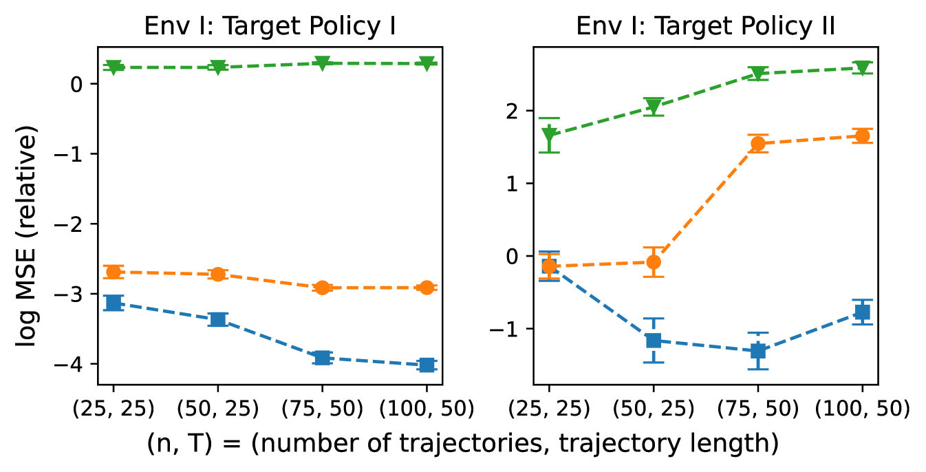
Figure 2 illustrates that our proposed method consistently achieves lower bias in policy evaluation across all settings. This improvement stems from leveraging the identification result in Theorem 3.1, which enables the recovery of lost information from unobserved variables by using reward-inducing proxies. In contrast, MDP-based methods typically exhibit higher bias and variance because they treat the observed state as the true state, even when the observed state is at best a noisy representation of the true state. Thus, these methods could easily lead to a biased estimate by ignoring the impact of unmeasured confounders.
For policy learning, we consider both Gaussian and Beta distribution policy class, and parameterize distribution parameters using either a linear basis or neural network. For Beta distribution policy class with a linear basis, we define , where is the state vector including an intercept, and with the same dimension as . For the neural network parameterization, we consider a one‐hidden‐layer MLP to approximate the in the Beta distributions. For Gaussian distribution policy class, the policy parameters are similarly parameterized by , where both the mean and standard deviation are approximated by either the same linear basis or neural network. While the neural network policy parameterization is capable of learning more complex optimal policies, the linear basis provides better interpretability and are often preferable in real-world applications.
To evaluate the performance of our proposed method, we apply Algorithm 2 and compare its results against the MDP and MDPW variants of the same approach, as well as against state-of-the-art policy learning algorithms including IQL, SAC, and CQL. To ensure a fair comparison, we employ the identical policy class for all policy parameterizations of the MDP and MDPW counterparts of our proposed method. Since IQL, SAC, and CQL are designed for deep reinforcement learning, we restrict their policy class to a Gaussian neural network. All data are generated using the synthetic environments and behavior policies described in the policy evaluation section, and Table 1 summarizes the averaged results over 50 simulation runs.
Table 1 indicates that our proposed method consistently outperforms competing approaches across varying sample sizes while maintaining comparable variance. This advantage is primarily due to the unbiased estimation of policy value at each iteration, which results in accurate policy gradients and ensures that policies are updated in the correct direction. In contrast, the MDP and MDPW variants of our method may suffer from biased estimation of the target policies, causing suboptimal policy updates and therefore poorer performance. Furthermore, methods originally designed for MDP settings (i.e., IQL, SAC, and CQL) directly solve the Bellman optimality equation, which does not hold in the presence of unmeasured confounders. As a result, these methods perform worse when unmeasured confounders are significant. Lastly, our proposed method achieves stable performance even with relatively small sample sizes, which is particularly desired in real-world applications where data can be limited.
| Method/(n, T) | (25, 25) | (50, 25) | (75, 50) | (100, 50) |
|---|---|---|---|---|
| Proposed-NN-Gaussian | 1.71 (0.43) | 1.80 (0.19) | 1.80 (0.16) | 1.77 (0.13) |
| Proposed-NN-Beta | 1.62 (0.36) | 1.68 (0.24) | 1.71 (0.13) | 1.72 (0.12) |
| Proposed-Linear-Gaussian | 1.66 (0.13) | 1.65 (0.09) | 1.68 (0.07) | 1.71 (0.07) |
| Proposed-Linear-Beta | 1.53 (0.11) | 1.55 (0.10) | 1.55 (0.09) | 1.58 (0.10) |
| MDPW-NN-Gaussian | 1.44 (0.29) | 1.41 (0.23) | 1.41 (0.20) | 1.33 (0.36) |
| MDPW-NN-Beta | 1.27 (0.38) | 1.34 (0.31) | 0.93 (0.43) | 0.95 (0.33) |
| MDPW-Linear-Gaussian | 1.41 (0.19) | 1.42 (0.12) | 1.41 (0.10) | 1.37 (0.10) |
| MDPW-Linear-Beta | 1.27 (0.14) | 1.28 (0.13) | 1.02 (0.58) | 0.98 (0.51) |
| MDPW-SAC | 0.72 (1.13) | 1.04 (0.34) | 1.23 (0.17) | 1.26 (0.15) |
| MDPW-CQL | 1.41 (0.39) | 1.44 (0.39) | 1.30 (0.32) | 1.29 (0.30) |
| MDPW-IQL | 0.61 (0.33) | 0.90 (0.21) | 0.94 (0.16) | 0.98 (0.13) |
| MDP-NN-Gaussian | 0.55 (0.39) | 0.10 (0.28) | -0.28 (0.10) | -0.18 (0.24) |
| MDP-NN-Beta | -0.21 (0.19) | -0.32 (0.10) | -0.24 (0.11) | -0.22 (0.17) |
| MDP-Linear-Gaussian | 0.86 (0.53) | 0.91 (0.48) | 1.08 (0.14) | 1.04 (0.12) |
| MDP-Linear-Beta | 0.46 (0.19) | 0.38 (0.09) | 0.11 (0.15) | 0.10 (0.21) |
| MDP-SAC | 0.22 (0.64) | 0.31 (0.34) | 0.28 (0.12) | 0.32 (0.10) |
| MDP-CQL | 0.44 (0.35) | 0.50 (0.27) | 0.41 (0.17) | 0.36 (0.18) |
| MDP-IQL | 0.29 (0.35) | 0.57 (0.25) | 0.66 (0.19) | 0.73 (0.14) |
In terms of the comparison between the neural network and linear policy classes, neural networks show better performance due to the richness of the function class, but the linear basis is capable of achieving comparable performance with fewer and more interpretable parameters, and thus may be of more interest in real-world applications, as demonstrated in Section 6.
6 Application to Pairfam Dataset
We applied our proposed method to the Panel Analysis of Intimate Relationships and Family Dynamics (Pairfam) dataset (Brüderl et al., 2023). Initiated in 2008, Pairfam is a comprehensive longitudinal dataset designed to explore the evolution of romantic relationships and family structures within Germany. For this study, we utilized the most recent release of the Pairfam dataset, which encompasses survey results from 14 waves (Brüderl et al., 2023). Given that the true feelings and thoughts of participants regarding their relationships are unobserved and survey responses are proxies for these sentiments, we treated the evolution of relationships as a confounded Partially Observable Markov Decision Process (POMDP). Our objective was to use the Pairfam dataset to estimate the optimal policy for maximizing long-term satisfaction in romantic relationships.
We define the immediate reward, , as the mean relationship satisfaction reported by the couple during each survey wave. The continuous action variable, , is selected as the frequency of sharing private feelings and communicating with partners, referred to as intimacy frequency. The observed state variables at each time point, , are represented by a 6-dimensional vector, which includes frequency of conflicts, frequency of appreciation, health status, future orientation of the couple, sexual satisfaction, and satisfaction with friendship of the couple. We defined the reward-proxy, , as a 4-dimensional vector that includes housing condition, household income, division of labor between the couple, and presence of relatives during the interview. Based on romantic relationship literature, all variables in could be considered as independent of when conditioned on observed states. To ensure data quality, we exclude samples with more than three missing values for any variable and applied matrix completion methods (Van Buuren and Groothuis-Oudshoorn, 2011) to impute the remaining missing data. Consequently, our refined dataset includes 809 trajectories () each with 14 time points ().
To conduct policy learning on the dataset, we consider both neural network and linear policy class as discussed in Section 5. We choose the same network structure as in Section 5, and the linear policy class is defined as , where and is a 7-dimensional vector that includes the intercept along with the 6 observed state variables discussed previously. For numerical stability, we constrain . The forms for are specifically selected for normalization purposes, enabling us to constrain the parameters associated with the beta distribution to be in the range , thus avoiding extremely large or small values that may result in abnormal policies.
We set the discount factor at = 0.9 and employ our proposed method to identify the optimal policy that maximizes long-term relationship satisfaction. To ensure robustness, each simulation randomly selects 400 trajectories as the training data and uses the remaining trajectories for testing data. Following Luckett et al. (2019), we use a Monte Carlo approximation of the policy value to evaluate performance of each method. Specifically, we train the policy on the training data and then apply our proposed policy evaluation method from Algorithm 1 to the testing set to evaluate the learned optimal policy, obtaining an estimate of the learned policy’s value. As shown in Figure 2, our proposed OPE method exhibits the smallest bias in the presence of unmeasured confounders compared to alternative methods.
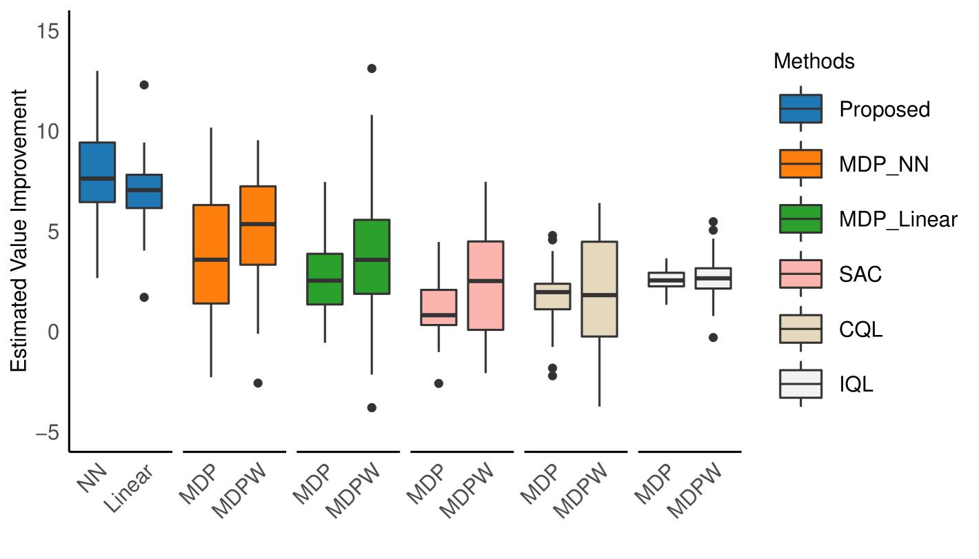
Figure 4 presents boxplots of the estimated policy values on both the training and testing sets for each method based on 100 simulation runs, with the baseline representing the observed discounted return. As shown in Figure 4, the proposed method achieves the best performance in terms of the improvement on policy value by taking unobserved confounders into account, which is consistent with the results presented in Section 5. In contrast, the MDP-based method tends to overestimate the policy value, which may be undesirable in safe-critical scenarios. Additionally, we observe that the linear policy class shows similar performance compared to the neural network policy class. Since the linear basis is more interpretable in such a setting, we further examine the learned optimal policy obtained using the linear policy class.
| Intercept | Conflicts | Appreciation | Health | Commitment | Sex | Friendship | |
|---|---|---|---|---|---|---|---|
| -0.0626 | -1.1602 | 1.4199 | 1.3774 | 1.1408 | 0.9960 | -0.2873 | |
| -0.8386 | 1.4781 | 0.1855 | -0.0315 | -0.7316 | 0.3191 | -0.6859 |
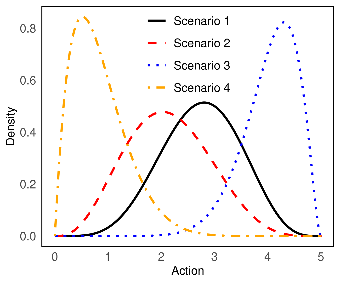
For linear policy class, the estimated values of are shown in Table 2, with and . To better illustrate the learned policy, we demonstrate the learned optimal policy under four different observed states. In romantic relationship studies, researchers have classified couples into different categories based on their commitment levels and couple dynamics (e.g., negative interactions) (Beckmeyer and Jamison, 2021). Thus, we chose commitment and conflict frequency as a proxy for couple dynamics. Consequently, we divided all the samples in the dataset into four categories based on whether their commitment and conflict levels are higher than the sample means, as shown in Table 3. It is important to note that all variables have been normalized to have mean 0 and variance 1. The values of observed state variables, other than conflicts and commitment, are selected as the sample means of those variables within each category. Figure 4 shows the induced optimal policy of each observed states.
| Scenarios | Conflicts | Appreciation | Health | Commitment | Sex | Friendship |
|---|---|---|---|---|---|---|
| Scenario 1 | 0.67 | -0.02 | 0.03 | 0.51 | 0.01 | 0.02 |
| Scenario 2 | -0.65 | -0.21 | -0.12 | -0.85 | -0.19 | -0.14 |
| Scenario 3 | -0.78 | 0.43 | 0.09 | 0.52 | 0.38 | 0.19 |
| Scenario 4 | 0.93 | -0.66 | -0.14 | -1.16 | -0.61 | -0.30 |
Figure 4 suggests that for couples experiencing a high frequency of conflicts and low levels of commitment (Scenario 4), fewer instances of sharing feelings and thoughts should be undertaken to improve satisfaction. In contrast, more frequent sharing is preferred for couples experiencing low conflicts and high commitment (Scenario 3). Additionally, moderate to high levels of sharing feelings and thoughts are preferred for couples with moderately high commitment and conflict levels (Scenario 1) and couples with moderately low commitment and conflict levels (Scenario 2). These results are consistent with the literature on the effects of sharing feelings and thoughts in romantic relationships. Although relationship researchers generally acknowledge the positive effects of sharing feelings (e.g., openness) (Ogolsky and Bowers, 2013), some studies have found that withholding feelings can be beneficial to relationship quality for individuals with high levels of social anxiety (Kashdan et al., 2007) and for couples with a more communal orientation (Le and Impett, 2013). Additionally, partner appreciation has been found to foster positive interactive dynamics through validation, thereby improving relationship satisfaction (Algoe, 2012).
7 Discussion
In this paper, we proposed a novel framework to conduct offline policy evaluation and policy learning on continuous action space with the existence of unmeasured confounder. We extended the proximal causal inference framework (Cui and Tchetgen Tchetgen, 2021) to an infinite horizon setting for the identification of policy value for a fixed target policy, and developed the corresponding minimax estimator. Based on the proposed estimator, we further developed a policy-gradient based method to search for the in-class optimal policy. The PAC bound of the proposed algorithm is provided to analyze its sample complexity.
Several improvements and extensions are worth exploring in the future. First, we assumed there is no coverage issue for the batch dataset. However, this assumption may not hold in real-world scenarios, such as medical applications where sample sizes are generally small and data is expensive to obtain. Thus, properly addressing the data coverage issue under the POMDP setting for both policy evaluation (Zhang and Jiang, 2024) and policy learning would be an interesting topic. Second, as demonstrated in real-data application, different observed state variables play various roles in formulating the policy. Meanwhile, conducting variable selection in an offline RL setting remains a challenging task, as there is no ground truth available for performance comparison. Systematically studying this problem would greatly improve the generalization of RL techniques. Finally, the proposed algorithm requires relatively large computation and memory resources due to the necessity of evaluating a new policy at each iteration. Therefore, developing a more efficient algorithm is desirable. A possible approach is to directly identify the policy gradient under the POMDP (Hong et al., 2023), however, such identification in continuous action space remains a challenge.
References
- Algoe (2012) Algoe, S. B. (2012), “Find, remind, and bind: The functions of gratitude in everyday relationships,” Social and personality psychology compass, 6, 455–469.
- Antos et al. (2008) Antos, A., Szepesvári, C., and Munos, R. (2008), “Learning near-optimal policies with Bellman-residual minimization based fitted policy iteration and a single sample path,” Machine Learning, 71, 89–129.
- Bach (2017) Bach, F. (2017), “Breaking the curse of dimensionality with convex neural networks,” The Journal of Machine Learning Research, 18, 629–681.
- Beckmeyer and Jamison (2021) Beckmeyer, J. J. and Jamison, T. B. (2021), “Identifying a typology of emerging adult romantic relationships: Implications for relationship education,” Family Relations, 70, 305–318.
- Bennett and Kallus (2023) Bennett, A. and Kallus, N. (2023), “Proximal reinforcement learning: Efficient off-policy evaluation in partially observed markov decision processes,” Operations Research.
- Bennett et al. (2021) Bennett, A., Kallus, N., Li, L., and Mousavi, A. (2021), “Off-policy evaluation in infinite-horizon reinforcement learning with latent confounders,” in International Conference on Artificial Intelligence and Statistics, PMLR, pp. 1999–2007.
- Bonvini and Kennedy (2022) Bonvini, M. and Kennedy, E. H. (2022), “Sensitivity analysis via the proportion of unmeasured confounding,” Journal of the American Statistical Association, 117, 1540–1550.
- Brüderl et al. (2023) Brüderl, J., Schmiedeberg, C., Castiglioni, L., Arránz Becker, O., Buhr, P., Fuß, D., Ludwig, V., Schröder, J., and Schumann, N. (2023), “The German Family Panel: Study Design and Cumulated Field Report (Waves 1 to 14),” .
- Brunke et al. (2022) Brunke, L., Greeff, M., Hall, A. W., Yuan, Z., Zhou, S., Panerati, J., and Schoellig, A. P. (2022), “Safe learning in robotics: From learning-based control to safe reinforcement learning,” Annual Review of Control, Robotics, and Autonomous Systems, 5, 411–444.
- Bruns-Smith (2021) Bruns-Smith, D. A. (2021), “Model-free and model-based policy evaluation when causality is uncertain,” in International Conference on Machine Learning, PMLR, pp. 1116–1126.
- Cai et al. (2021) Cai, H., Shi, C., Song, R., and Lu, W. (2021), “Jump interval-learning for individualized decision making,” arXiv preprint arXiv:2111.08885.
- Cai et al. (2022) Cai, Q., Yang, Z., and Wang, Z. (2022), “Reinforcement learning from partial observation: Linear function approximation with provable sample efficiency,” in International Conference on Machine Learning, PMLR, pp. 2485–2522.
- Chen and Qi (2022) Chen, X. and Qi, Z. (2022), “On well-posedness and minimax optimal rates of nonparametric q-function estimation in off-policy evaluation,” in International Conference on Machine Learning, PMLR, pp. 3558–3582.
- Chou et al. (2017) Chou, P.-W., Maturana, D., and Scherer, S. (2017), “Improving stochastic policy gradients in continuous control with deep reinforcement learning using the beta distribution,” in International conference on machine learning, PMLR, pp. 834–843.
- Cui et al. (2023) Cui, Y., Pu, H., Shi, X., Miao, W., and Tchetgen Tchetgen, E. (2023), “Semiparametric proximal causal inference,” Journal of the American Statistical Association, 1–12.
- Cui and Tchetgen Tchetgen (2021) Cui, Y. and Tchetgen Tchetgen, E. (2021), “A semiparametric instrumental variable approach to optimal treatment regimes under endogeneity,” Journal of the American Statistical Association, 116, 162–173.
- Dikkala et al. (2020) Dikkala, N., Lewis, G., Mackey, L., and Syrgkanis, V. (2020), “Minimax estimation of conditional moment models,” Advances in Neural Information Processing Systems, 33, 12248–12262.
- D’Haultfoeuille (2011) D’Haultfoeuille, X. (2011), “On the completeness condition in nonparametric instrumental problems,” Econometric Theory, 27, 460–471.
- Farahm et al. (2016) Farahm, A.-m., Ghavamzadeh, M., Szepesvári, C., and Mannor, S. (2016), “Regularized policy iteration with nonparametric function spaces,” Journal of Machine Learning Research, 17, 1–66.
- Fröhlich et al. (2018) Fröhlich, H., Balling, R., Beerenwinkel, N., Kohlbacher, O., Kumar, S., Lengauer, T., Maathuis, M. H., Moreau, Y., Murphy, S. A., Przytycka, T. M., et al. (2018), “From hype to reality: data science enabling personalized medicine,” BMC medicine, 16, 1–15.
- Fu et al. (2022) Fu, Z., Qi, Z., Wang, Z., Yang, Z., Xu, Y., and Kosorok, M. R. (2022), “Offline reinforcement learning with instrumental variables in confounded markov decision processes,” arXiv preprint arXiv:2209.08666.
- Fujimoto and Gu (2021) Fujimoto, S. and Gu, S. S. (2021), “A minimalist approach to offline reinforcement learning,” Advances in neural information processing systems, 34, 20132–20145.
- Fukumizu et al. (2009) Fukumizu, K., Gretton, A., Lanckriet, G., Schölkopf, B., and Sriperumbudur, B. K. (2009), “Kernel choice and classifiability for RKHS embeddings of probability distributions,” Advances in neural information processing systems, 22.
- Geer (2000) Geer, S. A. (2000), Empirical Processes in M-estimation, vol. 6, Cambridge university press.
- Guo et al. (2022) Guo, H., Cai, Q., Zhang, Y., Yang, Z., and Wang, Z. (2022), “Provably efficient offline reinforcement learning for partially observable markov decision processes,” in International Conference on Machine Learning, PMLR, pp. 8016–8038.
- Haarnoja et al. (2018) Haarnoja, T., Zhou, A., Hartikainen, K., Tucker, G., Ha, S., Tan, J., Kumar, V., Zhu, H., Gupta, A., Abbeel, P., et al. (2018), “Soft actor-critic algorithms and applications,” arXiv preprint arXiv:1812.05905.
- Hao et al. (2021) Hao, B., Ji, X., Duan, Y., Lu, H., Szepesvari, C., and Wang, M. (2021), “Bootstrapping fitted q-evaluation for off-policy inference,” in International Conference on Machine Learning, PMLR, pp. 4074–4084.
- Hoffman et al. (2011) Hoffman, M. W., Lazaric, A., Ghavamzadeh, M., and Munos, R. (2011), “Regularized least squares temporal difference learning with nested L2 and L1 penalization,” in European Workshop on Reinforcement Learning, Springer, pp. 102–114.
- Hong et al. (2023) Hong, M., Qi, Z., and Xu, Y. (2023), “A Policy Gradient Method for Confounded POMDPs,” arXiv preprint arXiv:2305.17083.
- Jin et al. (2020) Jin, C., Kakade, S., Krishnamurthy, A., and Liu, Q. (2020), “Sample-efficient reinforcement learning of undercomplete pomdps,” Advances in Neural Information Processing Systems, 33, 18530–18539.
- Kallus et al. (2022) Kallus, N., Mao, X., Wang, K., and Zhou, Z. (2022), “Doubly robust distributionally robust off-policy evaluation and learning,” in International Conference on Machine Learning, PMLR, pp. 10598–10632.
- Kallus and Uehara (2020) Kallus, N. and Uehara, M. (2020), “Statistically efficient off-policy policy gradients,” in International Conference on Machine Learning, PMLR, pp. 5089–5100.
- Kallus and Zhou (2020) Kallus, N. and Zhou, A. (2020), “Confounding-robust policy evaluation in infinite-horizon reinforcement learning,” Advances in neural information processing systems, 33, 22293–22304.
- Kallus and Zhou (2021) — (2021), “Minimax-Optimal Policy Learning Under Unobserved Confounding,” Management Science, 67, 2870–2890.
- Kashdan et al. (2007) Kashdan, T. B., Volkmann, J. R., Breen, W. E., and Han, S. (2007), “Social anxiety and romantic relationships: The costs and benefits of negative emotion expression are context-dependent,” Journal of Anxiety Disorders, 21, 475–492.
- Kostrikov et al. (2021) Kostrikov, I., Nair, A., and Levine, S. (2021), “Offline reinforcement learning with implicit q-learning,” arXiv preprint arXiv:2110.06169.
- Kress et al. (1989) Kress, R., Maz’ya, V., and Kozlov, V. (1989), Linear integral equations, vol. 82, Springer.
- Kumar et al. (2020) Kumar, A., Zhou, A., Tucker, G., and Levine, S. (2020), “Conservative q-learning for offline reinforcement learning,” Advances in Neural Information Processing Systems, 33, 1179–1191.
- Le and Impett (2013) Le, B. M. and Impett, E. A. (2013), “When Holding Back Helps: Suppressing Negative Emotions During Sacrifice Feels Authentic and Is Beneficial for Highly Interdependent People,” Psychological Science, 24, 1809–1815.
- Le et al. (2019) Le, H., Voloshin, C., and Yue, Y. (2019), “Batch policy learning under constraints,” in International Conference on Machine Learning, PMLR, pp. 3703–3712.
- Lee et al. (2018) Lee, K., Kim, S.-A., Choi, J., and Lee, S.-W. (2018), “Deep reinforcement learning in continuous action spaces: a case study in the game of simulated curling,” in International conference on machine learning, PMLR, pp. 2937–2946.
- Levine et al. (2020) Levine, S., Kumar, A., Tucker, G., and Fu, J. (2020), “Offline reinforcement learning: Tutorial, review, and perspectives on open problems,” arXiv preprint arXiv:2005.01643.
- Li et al. (2021) Li, J., Luo, Y., and Zhang, X. (2021), “Causal reinforcement learning: An instrumental variable approach,” arXiv preprint arXiv:2103.04021.
- Li et al. (2023) Li, Y., Zhou, W., and Zhu, R. (2023), “Quasi-optimal Reinforcement Learning with Continuous Actions,” in The Eleventh International Conference on Learning Representations.
- Liao et al. (2021) Liao, P., Klasnja, P., and Murphy, S. (2021), “Off-policy estimation of long-term average outcomes with applications to mobile health,” Journal of the American Statistical Association, 116, 382–391.
- Liao et al. (2022) Liao, P., Qi, Z., Wan, R., Klasnja, P., and Murphy, S. A. (2022), “Batch policy learning in average reward markov decision processes,” Annals of statistics, 50, 3364.
- Lillicrap et al. (2015) Lillicrap, T. P., Hunt, J. J., Pritzel, A., Heess, N., Erez, T., Tassa, Y., Silver, D., and Wierstra, D. (2015), “Continuous control with deep reinforcement learning,” arXiv preprint arXiv:1509.02971.
- Liu et al. (2018) Liu, Q., Li, L., Tang, Z., and Zhou, D. (2018), “Breaking the curse of horizon: Infinite-horizon off-policy estimation,” Advances in neural information processing systems, 31.
- Lu et al. (2022) Lu, M., Min, Y., Wang, Z., and Yang, Z. (2022), “Pessimism in the face of confounders: Provably efficient offline reinforcement learning in partially observable markov decision processes,” arXiv preprint arXiv:2205.13589.
- Luckett et al. (2019) Luckett, D. J., Laber, E. B., Kahkoska, A. R., Maahs, D. M., Mayer-Davis, E., and Kosorok, M. R. (2019), “Estimating dynamic treatment regimes in mobile health using v-learning,” Journal of the American Statistical Association.
- Miao et al. (2022) Miao, R., Qi, Z., and Zhang, X. (2022), “Off-policy evaluation for episodic partially observable markov decision processes under non-parametric models,” Advances in Neural Information Processing Systems, 35, 593–606.
- Miao et al. (2018) Miao, W., Geng, Z., and Tchetgen Tchetgen, E. J. (2018), “Identifying causal effects with proxy variables of an unmeasured confounder,” Biometrika, 105, 987–993.
- Mnih et al. (2015) Mnih, V., Kavukcuoglu, K., Silver, D., Rusu, A. A., Veness, J., Bellemare, M. G., Graves, A., Riedmiller, M., Fidjeland, A. K., Ostrovski, G., et al. (2015), “Human-level control through deep reinforcement learning,” nature, 518, 529–533.
- Newey and Powell (2003) Newey, W. K. and Powell, J. L. (2003), “Instrumental variable estimation of nonparametric models,” Econometrica, 71, 1565–1578.
- Ogolsky and Bowers (2013) Ogolsky, B. G. and Bowers, J. R. (2013), “A meta-analytic review of relationship maintenance and its correlates,” Journal of Social and Personal Relationships, 30, 343–367.
- Precup (2000) Precup, D. (2000), “Eligibility traces for off-policy policy evaluation,” Computer Science Department Faculty Publication Series, 80.
- Qi et al. (2023) Qi, Z., Miao, R., and Zhang, X. (2023), “Proximal learning for individualized treatment regimes under unmeasured confounding,” Journal of the American Statistical Association, 1–14.
- Shi et al. (2022a) Shi, C., Uehara, M., Huang, J., and Jiang, N. (2022a), “A minimax learning approach to off-policy evaluation in confounded partially observable markov decision processes,” in International Conference on Machine Learning, PMLR, pp. 20057–20094.
- Shi et al. (2022b) Shi, C., Zhang, S., Lu, W., and Song, R. (2022b), “Statistical inference of the value function for reinforcement learning in infinite-horizon settings,” Journal of the Royal Statistical Society Series B: Statistical Methodology, 84, 765–793.
- Shi et al. (2022c) Shi, C., Zhu, J., Ye, S., Luo, S., Zhu, H., and Song, R. (2022c), “Off-policy confidence interval estimation with confounded markov decision process,” Journal of the American Statistical Association, 1–12.
- Sutton and Barto (2018) Sutton, R. S. and Barto, A. G. (2018), Reinforcement learning: An introduction, MIT press.
- Tchetgen Tchetgen et al. (2020) Tchetgen Tchetgen, E., Ying, A., Cui, Y., Shi, X., and Miao, W. (2020), “An introduction to proximal causal learning,” arXiv preprint arXiv:2009.10982.
- Thomas and Brunskill (2016) Thomas, P. and Brunskill, E. (2016), “Data-efficient off-policy policy evaluation for reinforcement learning,” in International Conference on Machine Learning, PMLR, pp. 2139–2148.
- Uehara et al. (2020) Uehara, M., Huang, J., and Jiang, N. (2020), “Minimax weight and q-function learning for off-policy evaluation,” in International Conference on Machine Learning, PMLR, pp. 9659–9668.
- Uehara et al. (2024) Uehara, M., Kiyohara, H., Bennett, A., Chernozhukov, V., Jiang, N., Kallus, N., Shi, C., and Sun, W. (2024), “Future-dependent value-based off-policy evaluation in pomdps,” Advances in Neural Information Processing Systems, 36.
- Van Buuren and Groothuis-Oudshoorn (2011) Van Buuren, S. and Groothuis-Oudshoorn, K. (2011), “mice: Multivariate imputation by chained equations in R,” Journal of statistical software, 45, 1–67.
- Wang and Zou (2022) Wang, Y. and Zou, S. (2022), “Policy gradient method for robust reinforcement learning,” in International conference on machine learning, PMLR, pp. 23484–23526.
- Xie et al. (2019) Xie, T., Ma, Y., and Wang, Y.-X. (2019), “Towards optimal off-policy evaluation for reinforcement learning with marginalized importance sampling,” Advances in neural information processing systems, 32.
- Xu et al. (2023) Xu, Y., Zhu, J., Shi, C., Luo, S., and Song, R. (2023), “An instrumental variable approach to confounded off-policy evaluation,” in International Conference on Machine Learning, PMLR, pp. 38848–38880.
- Zhang and Bareinboim (2016) Zhang, J. and Bareinboim, E. (2016), “Markov decision processes with unobserved confounders: A causal approach,” Purdue AI Lab, West Lafayette, IN, USA, Tech. Rep.
- Zhang et al. (2020) Zhang, J., Kumor, D., and Bareinboim, E. (2020), “Causal imitation learning with unobserved confounders,” Advances in neural information processing systems, 33, 12263–12274.
- Zhang and Jiang (2024) Zhang, Y. and Jiang, N. (2024), “On the Curses of Future and History in Future-dependent Value Functions for Off-policy Evaluation,” arXiv preprint arXiv:2402.14703.
- Zhou (2024) Zhou, W. (2024), “Bi-Level Offline Policy Optimization with Limited Exploration,” Advances in Neural Information Processing Systems, 36.
- Zhou et al. (2024a) Zhou, W., Li, Y., and Zhu, R. (2024a), “Policy learning for individualized treatment regimes on infinite time horizon,” in Statistics in Precision Health: Theory, Methods and Applications, Springer, pp. 65–100.
- Zhou et al. (2023) Zhou, W., Li, Y., Zhu, R., and Qu, A. (2023), “Distributional shift-aware off-policy interval estimation: A unified error quantification framework,” arXiv preprint arXiv:2309.13278.
- Zhou et al. (2024b) Zhou, W., Zhu, R., and Qu, A. (2024b), “Estimating optimal infinite horizon dynamic treatment regimes via pt-learning,” Journal of the American Statistical Association, 119, 625–638.
- Zhu et al. (2020) Zhu, M., Wang, Y., Pu, Z., Hu, J., Wang, X., and Ke, R. (2020), “Safe, efficient, and comfortable velocity control based on reinforcement learning for autonomous driving,” Transportation Research Part C: Emerging Technologies, 117, 102662.