Relating by Contrasting: A Data-efficient
Framework for Multimodal DGMs
Abstract
Multimodal learning for generative models often refers to the learning of abstract concepts from the commonality of information in multiple modalities, such as vision and language. While it has proven effective for learning generalisable representations, the training of such models often requires a large amount of “related” multimodal data that shares commonality, which can be expensive to come by. To mitigate this, we develop a novel contrastive framework for generative model learning, allowing us to train the model not just by the commonality between modalities, but by the distinction between “related” and “unrelated” multimodal data. We show in experiments that our method enables data-efficient multimodal learning on challenging datasets for various multimodal variational autoencoder (VAE) models. We also show that under our proposed framework, the generative model can accurately identify related samples from unrelated ones, making it possible to make use of the plentiful unlabeled, unpaired multimodal data.
1 Introduction
To comprehensively describe concepts in the real world, humans collect multiple perceptual signals of the same object such as image, sound, text and video. We refer to each of these media as a modality, and a collection of different media featuring the same underlying concept is characterised as multimodal data. Learning from multiple modalities has been shown to yield more generalisable representations (Zhang et al., 2020; Guo et al., 2019; Yildirim, 2014), as different modalities are often complimentary in content while overlapping for common abstract concept.
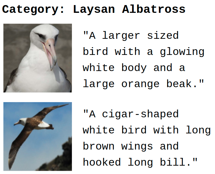
Despite the motivation, it is worth noting that the multimodal framework is not exactly data-efficient—constructing a suitable dataset requires a lot of “annotated” unimodal data, as we need to ensure that each multimodal pair is related in a meaningful way. The situation is worse when we consider more complicated multimodal settings such as language–vision, where one-to-one or one-to-many correspondence between instances of the two datasets are required, due to the difficulty in categorising data such that commonality amongst samples is preserved within categories. See Figure˜1 for an example from the CUB dataset (Welinder et al., a); although the same species of bird is featured in both image-caption pairs, their content differs considerably. It would be unreasonable to apply the caption from one to describe the bird depicted in the other, necessitating one-to-one correspondence between images and captions.
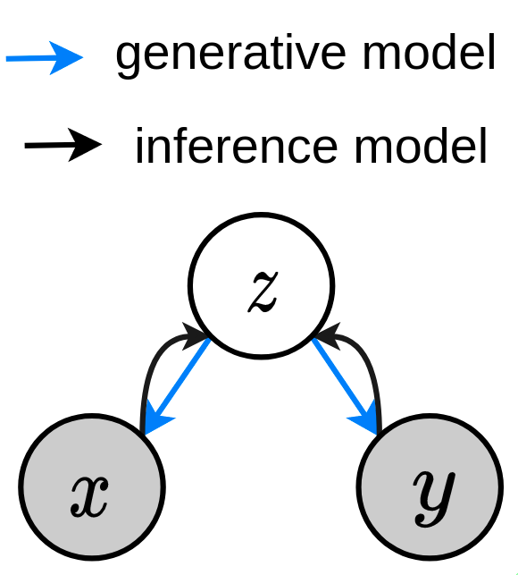
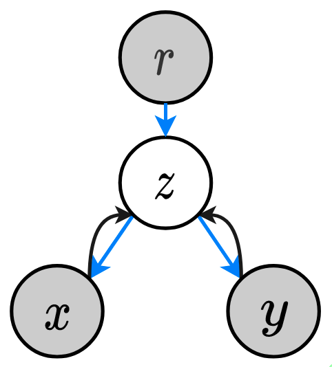
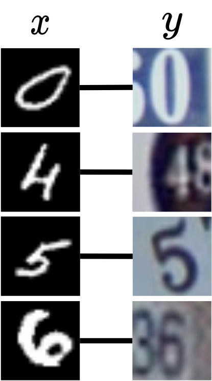
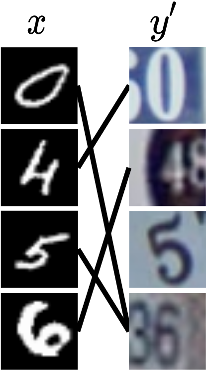
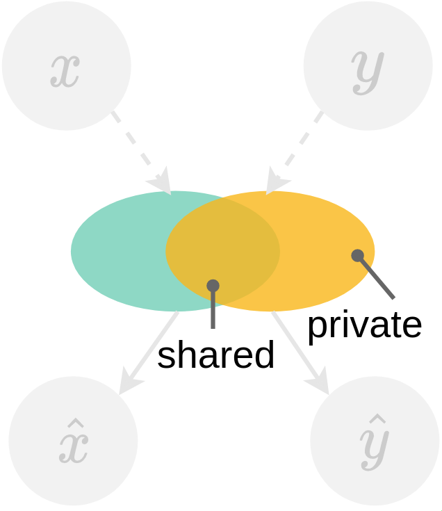
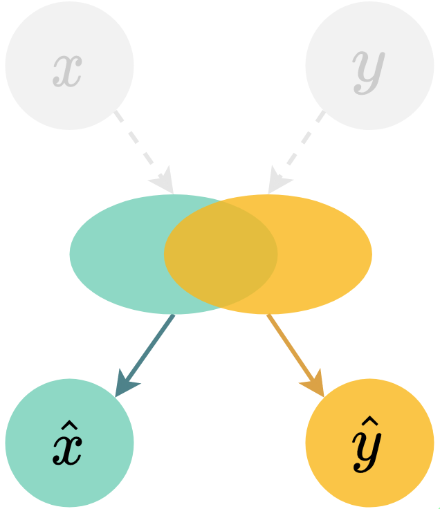
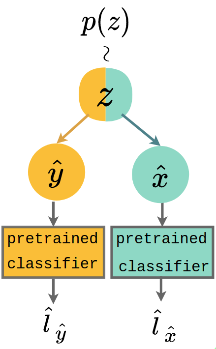
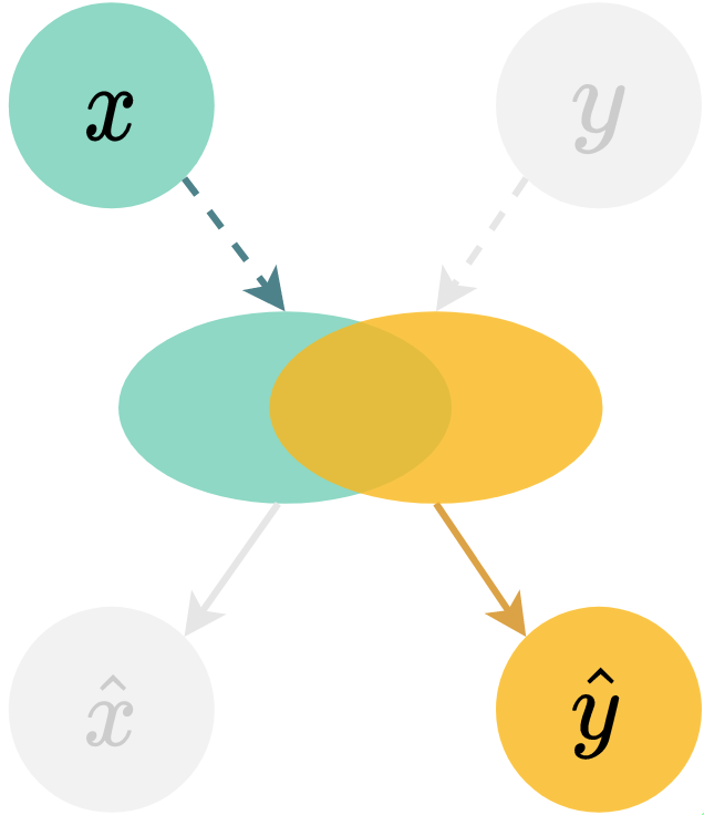
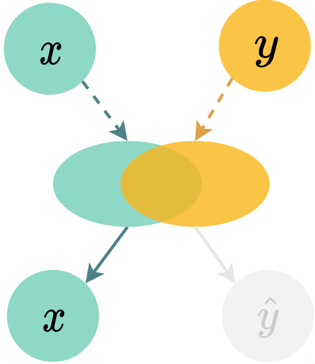
However, the scope of multimodal learning has been limited to leveraging the commonality between “related” pairs, while largely ignoring “unrelated” samples potentially available in any multimodal dataset—constructed through random pairing between modalities (Figure˜3). We posit that if a distinction can be established between the “related” and “unrelated” observations within a multimodal dataset, we could greatly reduce the amount of related data required for effective learning. Figure˜2 formalises this proposal. Multimodal generative models in previous work (Figure˜2(a)) typically assumes one latent variable that always generates related multimodal pair . In this work (Figure˜2(b)), we introduce an additional Bernoulli random variable that dictates the “relatedness” between and through , where and are related when , and unrelated when .
While can encode different dependencies, here we make the simplifying assumption that the Pointwise Mutual Information (PMI) between and should be high when , and low when . Intuitively, this can be achieved by adopting a max-margin metric. We therefore propose to train the generative moels with a novel contrastive-style loss (Hadsell et al., 2006; Weinberger et al., 2005), and demonstrate the effectiveness of our proposed method from a few different perspectives: Improved multimodal learning: showing improved multimodal learning for various state-of-the-art multimodal generative models on two challenging multimodal datasets. This is evaluated on four different metrics (Shi et al., 2019) summarised in §˜4.2; Data efficiency: learning generative models under the contrastive framework requires only of the data needed in baseline methods to achieve similar performance—holding true across different models, datasets and metrics; Label propagation: the contrastive loss encourages a larger discrepency between related and unrelated data, making it possible to directly identify related samples using the PMI between observations. We show that these data pairs can be used to further improve the learning of the generative model.
2 Related Work
Contrastive loss
Our work aims to encourage data-efficient multimodal generative-model learning using a popular representation learning metric—contrastive loss (Hadsell et al., 2006; Weinberger et al., 2005). There has been many successful applications of contrastive loss to a range of different tasks, such as contrastive predictive coding for time series data (van den Oord et al., 2018), image classification (Hénaff, 2020), noise contrastive estimation for vector embeddings of words (Mnih and Kavukcuoglu, 2013), as well as a range of frameworks such as DIM (Hjelm et al., 2019), MoCo (He et al., 2020), SimCLR (Chen et al., 2020) for more general visual-representation learning. The features learned by contrastive loss also perform well when applied to different downstream tasks — their ability to generalise is further analysed in (Wang and Isola, 2020) using quantifiable metrics for alignment and uniformity.
Contrastive methods have also been employed under a generative-model setting, but typically on generative adversarial networks (GANs) to either preserve or identify factors-of-variations in their inputs. For instance, SiGAN (Hsu et al., 2019) uses a contrastive loss to preserve identity for face-image hallucination from low-resolution photos, while (Yildirim et al., 2018) uses a contrastive loss to disentangle the factors of variations in the latent code of GANs. We here employ a contrastive loss in a distinct setting of multimodal generative model learning, that, as we will show with our experiments and analyses promotes better, more robust representation learning.
Multimodal VAEs
We also demonstrate that our approach is applicable across different approaches to learning multimodal generative models. To do so, we first summarise past work on multimodal VAE into two categories based on the modelling choice of approximated posterior :
-
a)
Explicit joint models: as single joint encoder .
Example work in this area include JMVAE (Suzuki et al., ), triple ELBO (Vedantam et al., 2018) and MFM (Tsai et al., 2019). Since the joint encoder require multimodal pair as input, these approaches typically require additional modelling components and/or inference steps to deal with missing modality at test time; in fact, all three approaches propose to train unimodal VAEs on top of the joint model that handles data from each modality independently.
-
b)
Factorised joint models: as factored encoders
This was first seen in Wu and Goodman (2018), as the MVAE model with defined as a product of experts (PoE), i.e. allowing for cross-modality generation without extra modelling components. Particularly, the MVAE caters to settings where data was not guaranteed to be always related, and where additional modalities were, in terms of information content, subsets of a primary data source—such as images and their class labels.
Alternately, Shi et al. (2019) explored an approach that explicitly leveraged the availability of related/paired data, motivated by arguments from embodied cognition of the world. They propose the MMVAE model, which additionally differs from the MVAE model in its choice of posterior approximation—where is modelled as the mixture of experts (MoE) of unimodal posteriors—to ameliorate shortcomings to do with precision miscalibration of the PoE. Furthermore, Shi et al. (2019) also posit four criteria that a multimodal VAE should satisfy, which we adopt in this work to evaluate the performance of our models.
Weakly-supervised learning
Using generative models for label propagation (see §˜4.5) is a form of weak supervision. Commonly seen approaches for weakly-supervised training with incomplete data include (1) graph-based methods (such as minimum cut) (Zhou et al., 2003; Zhu et al., 2003; Blum and Chawla, 2001), (2) low-density separation methods (Joachims, 1999; Burkhart and Shan, 2020) and (3) disagreement-based models (Blum and Mitchell, 1998; Zhou and Li, 2005; 2010). However, (1) and (2) suffers from scalability issues due to computational inefficiency and optimisation complexity, while (3) works well for many different tasks but requires training an ensemble of learners.
The use of generative models for weakly supervised learning has also been explored in Nigam et al. (2000); Miller and Uyar (1996), where labels are estimated using expectation-maximisation (EM) (Dempster et al., 1977) for instances that are unlabelled. Notably, models trained with our contrastive objective does not need EM to leverage unlabelled data (see §˜4.5) to determine the relatedness of two examples we only need to compute a threshold (estimation of PMI) using the trained model.
3 Methodology
Given data over observations from two modalties , one can learn a multimodal VAE targetting , where are deep neural networks (decoders) parametrised by . To maximise the joint marginal likelihood , one approximates the intractable model posterior with a variational posterior , allowing us to optimise a variational evidence lower bound (ELBO), defined as This leaves open the question of how to model the approximatd posterior . As mentioned in §˜2, there are two schools of thinking, namely explicit joint model such as JMVAE (Suzuki et al., ) and factorised joint model including MVAE (Wu and Goodman, 2018) and MMVAE (Shi et al., 2019). In this work we demonstrate the effectiveness of our approach across all these models.
3.1 Contrastive loss for “relatedness” learning
Where prior work always assumes to be related, we introduce a relatedness variable explicitly capturing this aspect. Our approach is motivated by the characteristics of pointwise mutual information (PMI) between related and unrelated observations across modalities:
Hypothesis 3.1.
Let be a related data pair from two modalities, and let denote a data point unrelated to . Then, the pointwise mutual information .
Note that the PMI measures the statistical dependence between values , which for a joint distribution is defined as . Hypothesis 3.1 should be a fairly uncontroversial assumption for true generative models: we say simply that under the joint distribution for related data , the PMI between related points is stronger than that between unrelated points . In fact, we demonstrate in §˜4.5 that for a well-trained generative model, PMI is a good indicator of relatedness, enabling pairing of random multimodal data by thresholding the PMI estimated by the trained model. It is therefore possible to leverage relatedness while training parametrised generative model by maximising the difference in PMI between related and unrelated pairs, i.e. . We show in Appendix˜A that this is equivalent to maximising the difference between the joint marginal likelihoods of related and unrelated pairs (Figure˜3(a) and 3(b)). This casts multimodal learning as max-margin optimisation, with the contrastive (triplet) loss as a natural choice of objective: Intuitively, attempts to make distance between a positive pair smaller than the distance between a negative pair by margin . We adopt this loss to our objective by omitting margin and replacing with the (negative) joint marginal likelihood . Following Song et al. (2016), with negative samples , we have
| (1) |
We choose to put the sum over within the following conventions in previous work on contrastive loss (van den Oord et al., 2018; Hjelm et al., 2019; Chen et al., 2020). As the loss is asymmetric, one can average over and to ensure negative samples in both modalities are accounted for—giving our contrastive objective:
| (2) |
Note that since only the joint marginal likelihood terms are needed in Equation˜2, the contrastive learning framework can be directly applied to any multimodal generative model without needing extra components. We also show our contrastive framework applies when the number of modalities is more than two (cf. Appendix˜C).
Dissecting
Although similar to the VAE LABEL:eq:elbo, our objective eq.˜2 directly maximises in . by itself is not a effective objective as in minimises , which can overpower the effect of during training.
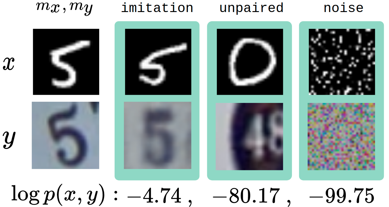
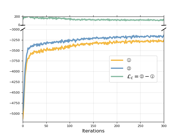
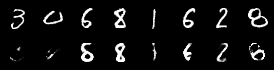
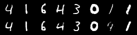
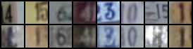
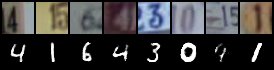
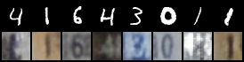
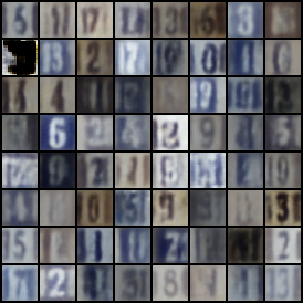
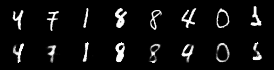
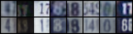
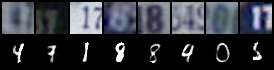
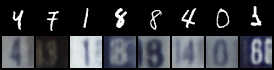
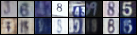
We intuit this phenomenon using a simple example in Figure˜4 with natural images, showing the log likelihood of in column 2, 3, 4 (green) on a Gaussian distribution , with the images in the first column of Figure˜4 as means and with constant variance . While achieving high requires matching (col 2), we see both unrelated digits (col 3) and noise (col 4) can lead to (comparatively) poor joint log likelihoods. This indicates that the generative model need not generate valid, unrelated images to minimise —generating noise would have roughly the same effect on log likelihood. As a result, the model can trivially minimise by generating noise that minimises instead of accurate reconstruction that maximises .
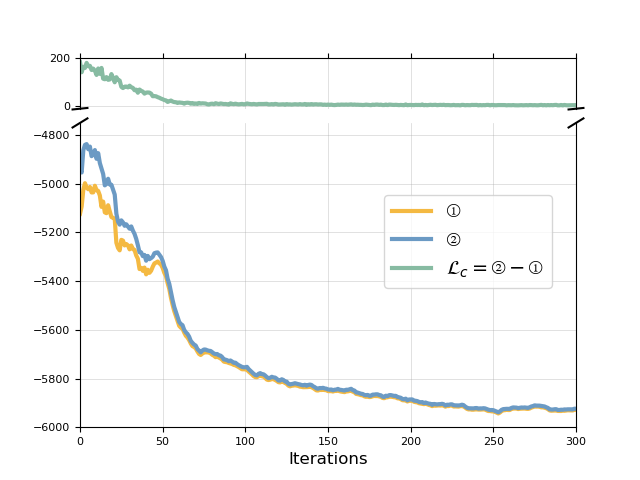
This learning dynamic is verified empirically, as we show in Figure˜9 in Appendix˜D: optimising by itself results in the loss approaching 0 within the first 100 iterations, and both and takes on extremely low values, resulting in a model that generates random noise.
Final objective
To mitigate this issue, we need to ensure that minimising does not overpower maximising . We hence introduce a hyperparameter on to upweight the maximisation of the marginal likelihood, with the final objective to minimise
| (3) |
We conduct ablation studies on the effect of in Appendix˜E, noting that larger encourages better quality of generation and more stable training in some cases, while models trained with smaller are better at predicting “relatedness” between multimodal samples. We also note that optimising Equation˜3 maximises the pointwise mutual information ; see Appendix˜B for a proof.
3.2 Optimising the objective
Since in VAEs we do not have access to the exact marginal likelihood, we have to optimise an approximated version of the true contrastive objective in Equation˜3. In Equation˜4 we list a few possible candidates of estimators and their relationships to the (log) joint marginal likelihood:
| (4) |
with the ELBO from Eq. LABEL:eq:elbo, the importance weighted autoencoder (IWAE), a -sample lower bound estimator that can compute an arbitrarily tight bound with increasing (Burda et al., 2016), and the upper bound (CUBO), an upper-bound estimator (Dieng et al., 2017).
We now discuss our choice of approximation of for each term in equation Equation˜3:
-
Minimising this term maximises the joint marginal likelihood, which can hence be approximated with a valid lower-bound estimator Equation˜4; the IWAE estimator being the preferred choice.
-
For this term, we consider two choices of estimators:
-
1)
CUBO: Since of Equation˜3 minimises the joint marginal likelihoods, to ensure an upper-bound estimator to in eq.˜3, we need to employ an upper-bound estimator. Here we propose to use CUBO in Equation˜4. While such a bounded approximation is indeed desirable, existing upper-bound estimators tend to have rather large bias/variance and can therefore yield poor quality approximations.
-
2)
IWAE: We therefore also propose to estimate with the IWAE estimator, as it provides an arbitrarily tight, low variance lower-bound (Burda et al., 2016) to . Although this no longer ensure a valid bound on the objective, we hope that having a more accurate approximation to the marginal likelihood (and by extension, the contrastive loss) can affect the performance of the model positively.
We report results using both IWAE and CUBO estimators in §˜4, denoted cI and cC respectively.
-
1)
4 Experiments
As stated in §˜1, we analyse the suitability of contrastive learning for multimodal generative models from three persepctives—improved multimodal learning (§˜4.3), data efficiency (§˜4.4) and label propagation (§˜4.5). Throughout the experiments, we take negative samples for the contrastive objective, set based on analyses of ablations in appendix˜E, and take samples for our IWAE estimators. We now introduce the datasets and metrics used for our experiments.
4.1 Datasets
MNIST-SVHN
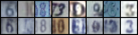
The dataset is designed to separate conceptual complexity, i.e. digit, from perceptual complexity, i.e. color, style, size. Each data pair contains 2 samples of the same digit, one from each dataset (see examples in Figure˜3(a)). We construct the dataset such that each instance from one dataset is paired with instances of the same digit from the other dataset. Although both datasets are simple and well-studied, the many-to-many pairing between samples creates matching of different writing styles vs. backgrounds and colors, making it a challenging multimodal dataset.
CUB Image-Captions
We also consider a more challenging language-vision multimodal dataset, Caltech-UCSD Birds (CUB) (Welinder et al., b; Reed et al., 2016). The dataset contains 11,788 photos of birds, paired with captions describing the bird’s physical characteristics, collected through Amazon Mechanical Turk (AMT). See CUB image-caption pair in Figure˜1.
4.2 Metrics
Shi et al. (2019) proposed four criteria for multimodal generative models (§˜4.2, left), that we summarise and unify as metrics to evaluate these criteria for different generative models (§˜4.2, right). We now introduce each criterion and its corresponding metric in detail.
Criterion Metric
Criterion Metric
Criterion Metric
Criterion Metric
(a) Latent accuracy (§˜4.2)
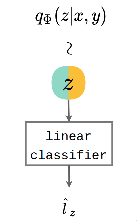
Criterion: latent space factors into “shared” and “private” subspaces across modalities. We fit a linear classifier on the samples from to classify the information shared between the two modalities. For MNIST-SVHN, this can be the digit label as shown in §˜4.2 (right). We check if is the same as the digit label of the original inputs and , with the intuition that extracting the commonality between and from latent representation using a linear transform, supports the claim that the latent space has factored as desired.
(b) Joint coherence (§˜4.2)
Criterion: model generates paired samples that preserves the commonality observed in data. Again taking MNIST-SVHN as an example, this can be verified by taking pre-trained MNIST and SVHN digit classifiers and applying them on the multimodal observations generated from the same prior sample . Coherence is computed by how often generations and classify to the same digit, i.e. whether .
(c) Cross coherence (§˜4.2)
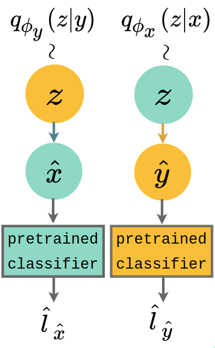
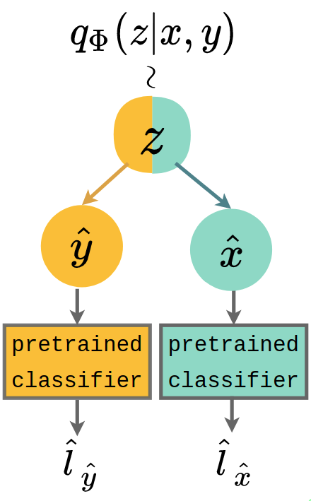
Criterion: model generates data in one modality conditioned on the other while preserving shared commonality. To compute cross coherence, we generate observations using latent from unimodal marginal posterior and from . Similar to joint coherence, the criterion here is evaluated by predicting the label of the cross-generated samples , using off-the-shelf MNIST and SVHN classifiers. In §˜4.2 (right), the cross coherence is the frequency of which and .
(d) Synergy coherence (§˜4.2)
Criterion: models learnt across multiple modalities should be no worse than those learnt from just one. For consistency, we evaluate this criterion from a coherence perspective. Given generations and from , we again examine if generated and original labels match; i.e. if .
See Appendix˜F for details on architecture. All quantitative results are reported over 5 runs. In addition to these quantitative metrics, we also showcase the qualitative results on both datasets in Appendix˜G and Appendix˜H.
4.3 Improved multimodal learning
Finding: Contrastive learning improves multimodal learning across all models and datasets.
MNIST-SVHN
See Table˜1 (top, 100% data used) for results on the full MNIST-SVHN dataset. Note that for MMVAE, since the joint posterior is factorised as the mixture of unimodal posteriors and , the model never directly takes sample from the explicit form of the joint posterior. Instead, it takes equal number of samples from each unimodal posteriors, reflective of the equal weighting of the mixture. As a result, it is not meaningful to compute synergy coherence for MMVAE as it is exactly the same as the coherence of any single-way generation.
From Table˜1 (top, 100% data used), we see that models trained on our contrastive objective (cI-<MODEL> and cC-<MODEL>) improves multimodal learning performance significantly for all three generative models evaluated on the metrics. The results showcase the robustness of our approach from the perspectives of modelling choice and metric of interests. In particular, note that for the best performing model MMVAE, using IWAE estimator for of Eq Equation˜3 (cI-MMVAE) yields slightly better results than CUBO (cC-MMVAE), while for the two other models the performance for different estimators are similar.
We also include qualitative results for MNIST-SVHN, including generative results, marginal likelihood table and diversity analysis in Appendix˜G.
| Data | Methods | Latent accuracy () | Joint [-2pt] Coherence () | Cross coherence () | Synergy coherence () | ||||
| M | S | SM | MS | jointM | jointS | ||||
| 100% of data used | MMVAE | 92.48 (0.37) | 79.03 (1.17) | 42.32 (2.97) | 70.77 (0.35) | 85.50 (1.05) | — | — | |
| cI-MMVAE | 93.97 (0.36) | 81.87 (0.52) | 43.94 (0.96) | 79.66 (0.59) | 92.67 (0.29) | — | — | ||
| cC-MMVAE | 93.10 (0.17) | 80.88 (0.80) | 45.46 (0.78) | 79.34 (0.54) | 92.35 (0.46) | — | — | ||
| MVAE | 91.65 (0.17) | 64.12 (4.58) | 9.42 (7.82) | 10.98 (0.56) | 21.88 (2.21) | 64.60 (9.25) | 52.91 (8.11) | ||
| cI-MVAE | 96.97 (0.84) | 75.94 (6.20) | 15.23 (10.46) | 10.85 (1.17) | 27.70 (2.09) | 85.07 (7.73) | 75.67 (4.13) | ||
| cC-MVAE | 97.42 (0.40) | 81.07 (2.03) | 8.85 (3.86) | 12.83 (2.25) | 30.03 (2.46) | 75.25 (5.31) | 69.42 (3.94) | ||
| JMVAE | 84.45 (0.87) | 57.98 (1.27) | 42.18 (1.50) | 49.63 (1.78) | 54.98 (3.02) | 85.77 (0.66) | 68.15 (1.38) | ||
| cI-JMVAE | 84.58 (1.49) | 64.42 (1.42) | 48.95 (2.31) | 58.16 (1.83) | 70.61 (3.13) | 93.45 (0.52) | 84.00 (0.97) | ||
| cC-JMVAE | 83.67 (3.48) | 66.64 (2.92) | 47.27 (4.52) | 59.73 (3.85) | 69.49 (2.19) | 91.21 (6.59) | 84.07 (3.19) | ||
| 20% of data used | MMVAE | 88.54 (0.37) | 68.90 (1.79) | 37.71 (0.60) | 59.52 (0.28) | 76.33 (2.23) | — | — | |
| cI-MMVAE | 91.64 (0.06) | 73.02 (0.80) | 42.74 (0.36) | 69.51 (1.18) | 86.75 (0.28) | — | — | ||
| cC-MMVAE | 92.10 (0.19) | 71.29 (1.05) | 40.77 (0.93) | 68.43 (0.90) | 86.24 (0.89) | — | — | ||
| MVAE | 90.29 (0.57) | 33.44 (0.26) | 10.88 (9.15) | 8.72 (0.92) | 12.12 (3.38) | 42.10 (5.22) | 44.95 (5.92) | ||
| cI-MVAE | 93.72 (1.09) | 56.74 (7.97) | 12.79 (6.82) | 14.18 (2.19) | 20.23 (4.55) | 75.36 (5.05) | 64.81 (4.81) | ||
| cC-MVAE | 92.74 (2.97) | 52.99 (8.35) | 17.95 (12.52) | 14.70 (1.65) | 24.90 (5.77) | 56.86 (18.84) | 54.28 (9.86) | ||
| JMVAE | 77.53 (0.13) | 52.55 (2.18) | 26.37 (0.54) | 42.58 (5.32) | 41.44 (2.26) | 85.07 (9.74) | 51.95 (2.28) | ||
| cI-JMVAE | 77.57 (4.02) | 57.91 (1.28) | 32.58 (5.89) | 51.85 (1.27) | 47.92 (10.32) | 92.54 (1.13) | 67.01 (8.72) | ||
| cC-JMVAE | 81.11 (2.76) | 57.85 (2.23) | 34.00 (7.18) | 50.73 (0.45) | 56.89 (6.18) | 88.36 (4.38) | 68.49 (8.82) | ||
CUB
Following Shi et al. (2019), for the images in CUB, we observe and generate in feature space instead of pixel space by preprocessing the images using a pre-trained ResNet-101 (He et al., 2016). A nearest-neighbour lookup among all the features in the test set is used to project the feature generations of the model back to image space. This helps circumvent CUB image complexities to some extent—as the primary goal here is to learn good models and representations of multimodal data, rather than a focus on pixel-level image quality of generations.
The metrics listed in §˜4.2 can also be applied to CUB with some modifications. Since bird-species classes are disjoint for the train and test sets, and as we show in Figure˜1 contains substantial in-class variance, it is not constructive to evaluate these metrics using bird categories as labels. In Shi et al. (2019), the authors propose to use Canonical Correlation Analysis (CCA)—used by Massiceti et al. as a reliable vision-language correlation baseline—to compute coherence scores between generated image-caption pairs; which we employ (i.e. (b), (c), (d) in §˜4.2) for CUB.
We show the results in Table˜2 (top, 100% data used). We see that our contrastive approach (both cI-<MODEL> and cC-<MODEL>) is even more effective on this challenging vision-language dataset, with significant improvements to the correlation of generated image-caption pairs. It is also on this more complicated dataset where the advantages of using the stable, low-variance IWAE estimator are highlighted — for both MVAE and JMVAE, the contrastive objective with CUBO estimator suffers from numerical stability issues, yielding close-to-zero correlations for all metrics in Table˜2. Results for these models are therefore omitted.
We also show the qualitative results for CUB in Appendix˜H.
| Data | Methods | Joint [-2pt] Coherence (CCA) | Cross coherence (CCA) | Synergy coherence (CCA) | |||
| imgcap | cap img | jointimg | jointcap | ||||
| 100% of data used | MMVAE | 0.212 (2.94e-2) | 0.154 (7.05e-3) | 0.244 (5.83e-3) | - | - | |
| cI-MMVAE | 0.314 (3.12e-2) | 0.188 (4.02e-3) | 0.334 (1.20e-2) | - | - | ||
| cC-MMVAE | 0.263 (1.47e-2) | 0.244 (2.24e-2) | 0.369 (3.18e-3) | - | - | ||
| MVAE | 0.075 (8.71e-2) | -0.008 (1.41e-4) | 0.000 (1.84e-3) | -0.002 (4.95e-3) | 0.001 (1.13e-3) | ||
| cI-MVAE | 0.209 (3.12e-2) | 0.247 (1.12e-4) | -0.008 (3.99e-4) | 0.218 (5.27e-3) | 0.148 (9.23e-3) | ||
| JMVAE | 0.220 (1.19e-2) | 0.157 (4.98e-2) | 0.191 (3.11e-2) | 0.212 (1.23e-2) | 0.143 (1.14e-1) | ||
| cI-JMVAE | 0.255 (3.24e-3) | 0.149 (1.25e-3) | 0.226 (7.48e-2) | 0.202 (1.12e-4) | 0.176 (6.23e-2) | ||
| 20% of data used | MMVAE | 0.117 (1.51e-2) | 0.094 (7.21e-3) | 0.153 (1.47e-2) | - | - | |
| cI-MMVAE | 0.206 (1.65e-2) | 0.136 (1.51e-2) | 0.251 (2.39e-2) | - | - | ||
| cC-MMVAE | 0.226 (4.69e-2) | 0.188 (2.80e-2) | 0.273 (8.67e-3) | - | - | ||
| MVAE | 0.091 (2.63e-2) | 0.008 (4.81e-3) | 0.005 (7.50e-3) | 0.020 (8.77e-3) | 0.009 (1.17e-2) | ||
| cI-MVAE | 0.132 (3.33e-2) | 0.192 (3.91e-2) | -0.002 (3.61e-3) | 0.162 (7.89e-2) | 0.081 (3.82e-2) | ||
| JMVAE | 0.127 (3.76e-2) | 0.118 (3.82e-3) | 0.154 (8.34e-3) | 0.181 (1.26e-2) | 0.139 (1.33e-2) | ||
| cI-JMVAE | 0.269 (1.20e-2) | 0.134 (4.24e-4) | 0.210 (2.35e-2) | 0.192 (1.41e-4) | 0.168 (3.82e-3) | ||
4.4 Data Efficiency
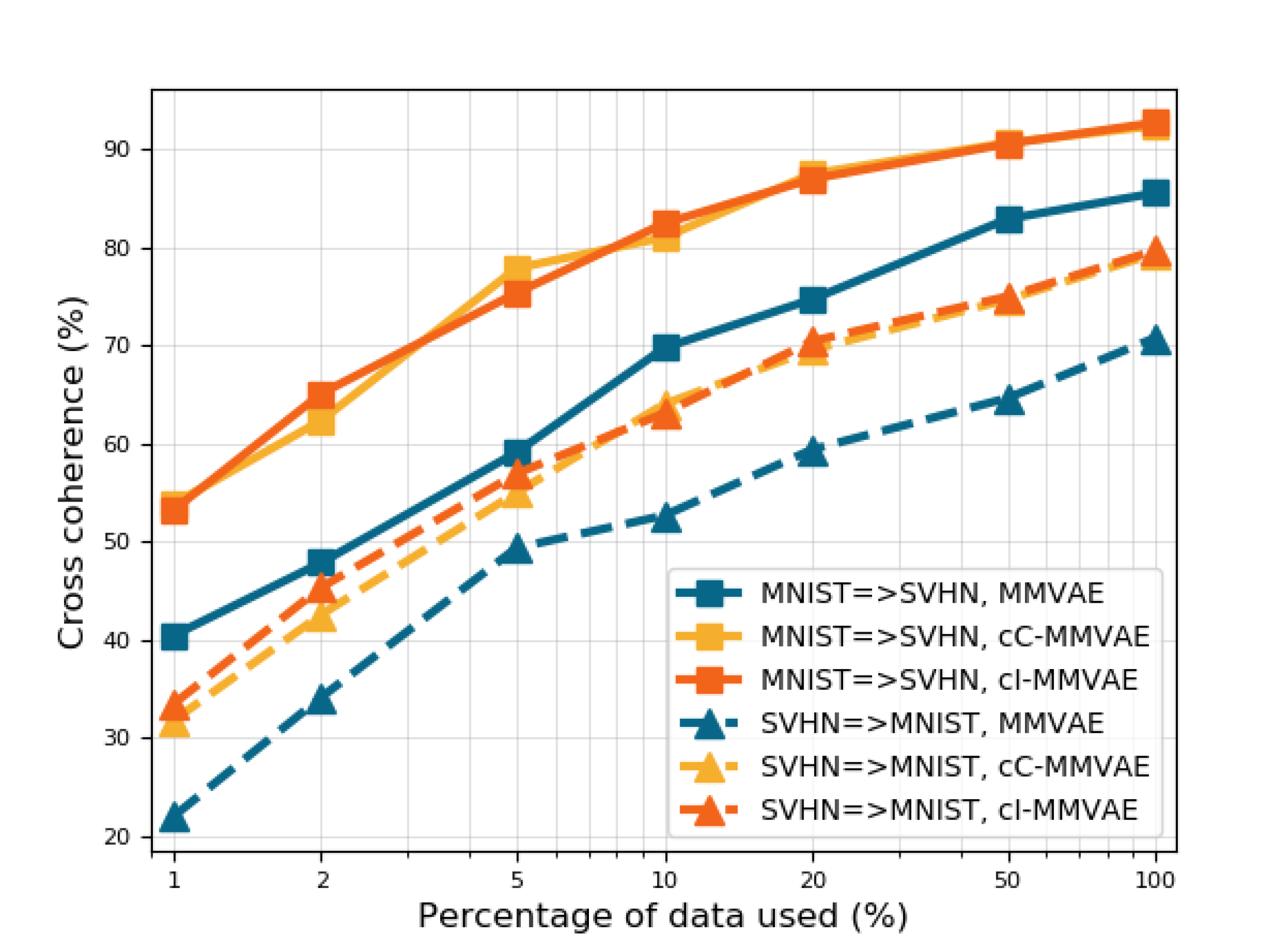
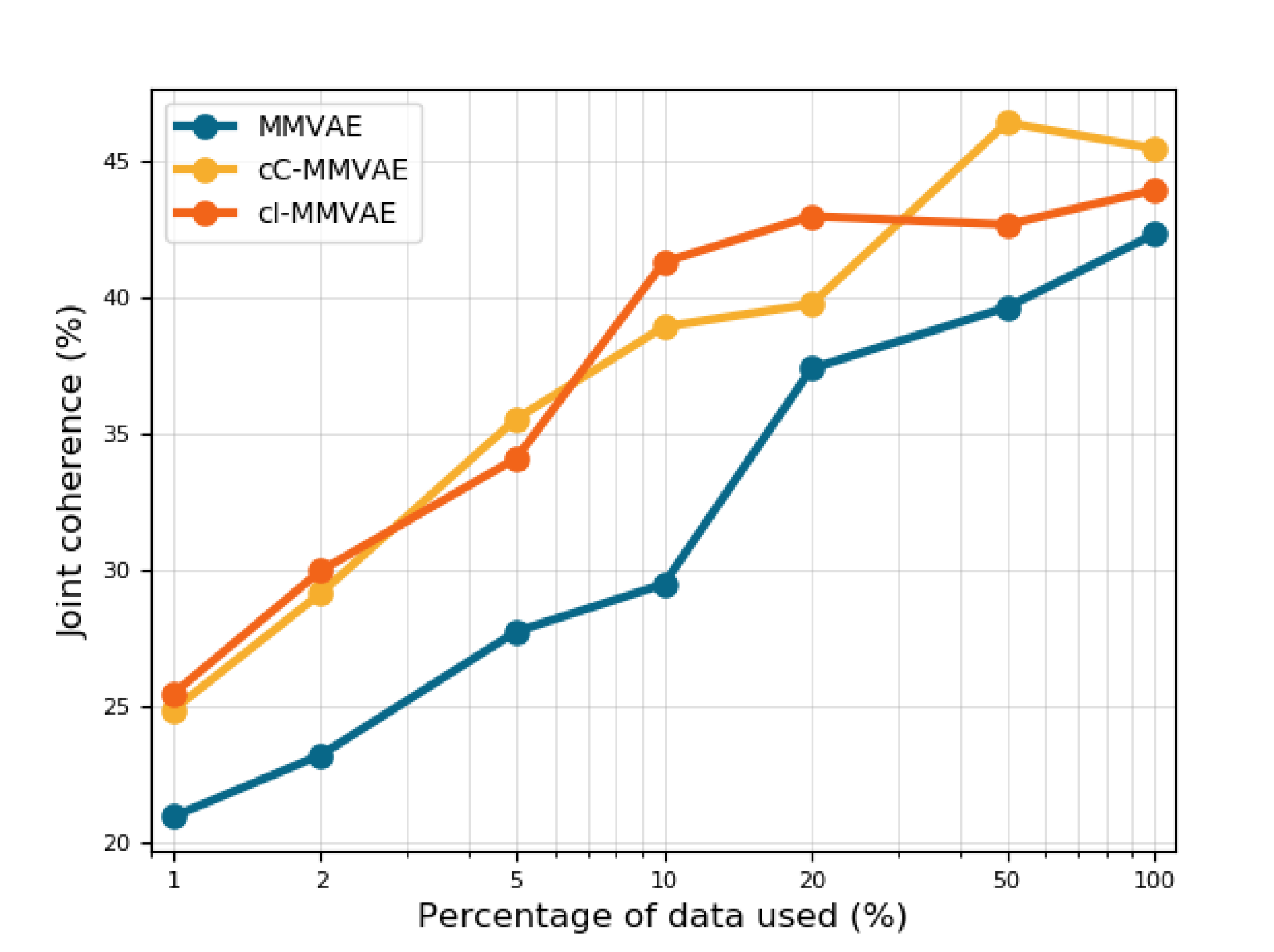
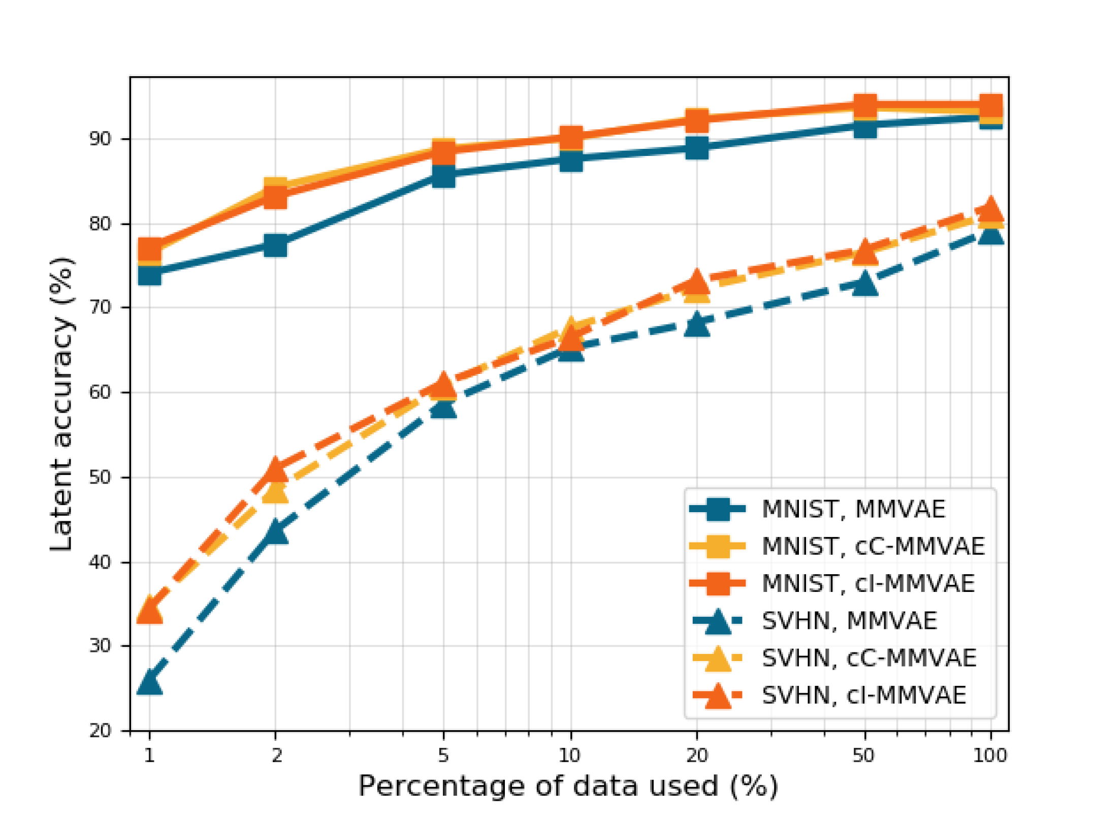
Finding: Contrastive learning on 20% of data matches baseline models on full data.
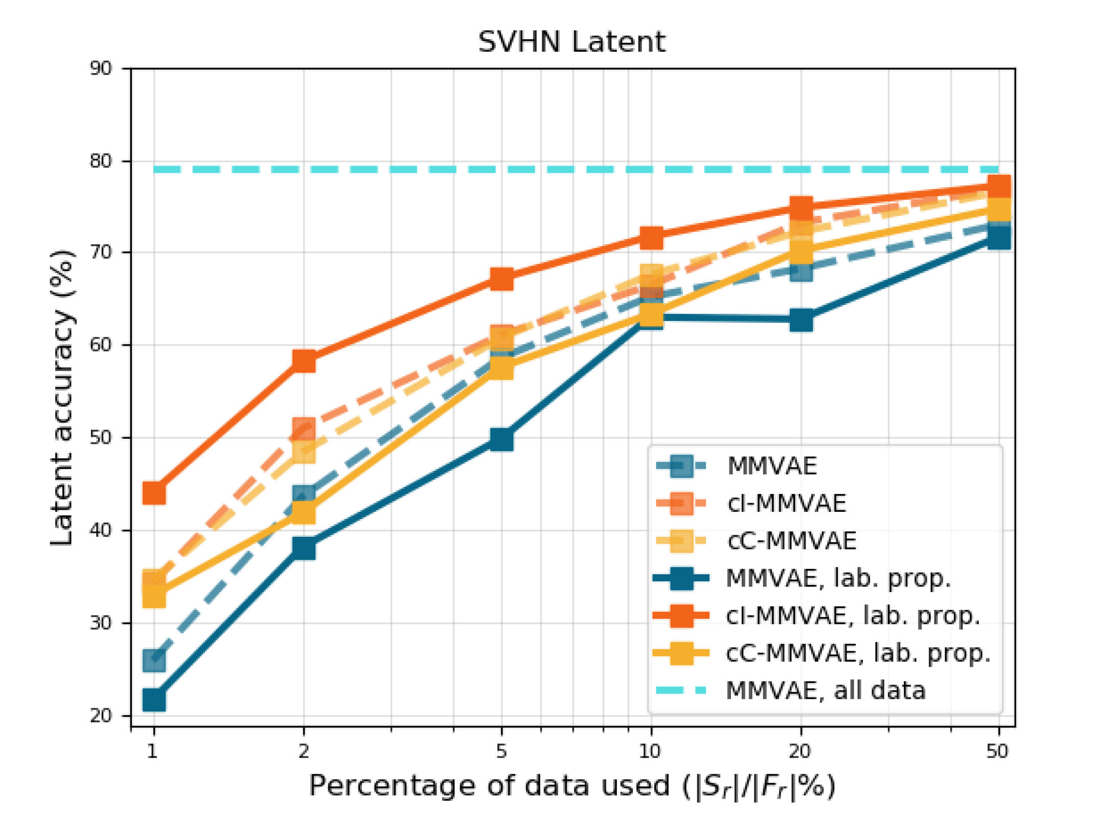
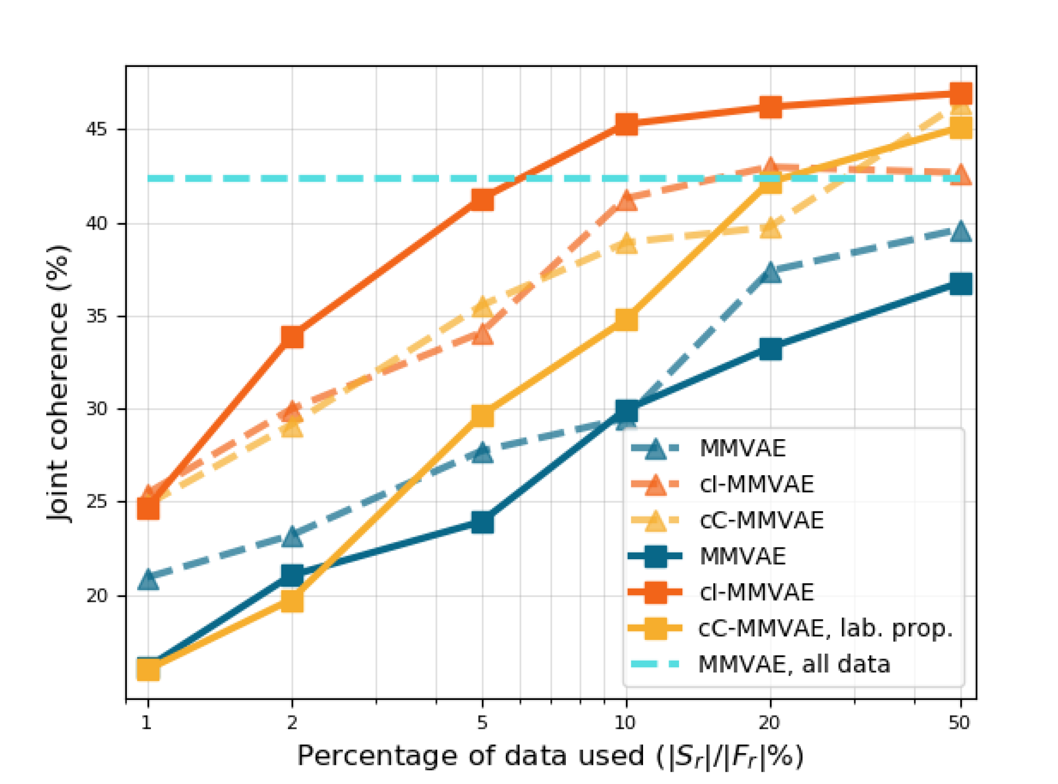
We plot the quantitative performance of MMVAE with and without contrastive learning against the percentage of the original dataset used, as seen in Figure˜6. We observe that the performance of contrastive MMVAE with the IWAE (cI-MMVAE, red) and CUBO estimators (cC-MMVAE, yellow) are consistently better than the baselines (MMVAE, blue), and that baseline performance using all related data is matched by the contrastive MMVAE using just 10—20% of data. The partial datasets used here are constructed by first taking % of each unimodal dataset, then pairing to create multimodal datasets (§˜4.1)—ensuring it contains the requisite amount of “related” samples.
In addition, we reproduce results generated from using 100% of the data in MNIST-SVHN and CUB (Tables˜1 and 2) using only 20% of the original multimodal datasets (Tables˜1 and 2 (bottom)). Comparing results between top vs. bottom in Tables˜1 and 2 shows that this finding holds across the models, on both MNIST-SVHN and CUB datasets. This shows that the efficiency gains from a contrastive approach is invariant to VAE type, data, and metrics used, underscoring its effectiveness.
4.5 Label propagation
Finding: Generative models learned contrastively are good predictors of “relatedness”, enabling label propagation and matching baseline performance on full datasets, using only 10% of data.
Here, we show that our contrastive framework encourages a larger discrepancy between the PMI of related vs. unrelated data, as set out in ˜3.1, allowing one to first train the model on a small subset of related data, and subsequently construct a classifier using PMI that identifies related samples in the remaining data. We now introduce our pipeline for label propagation in details.
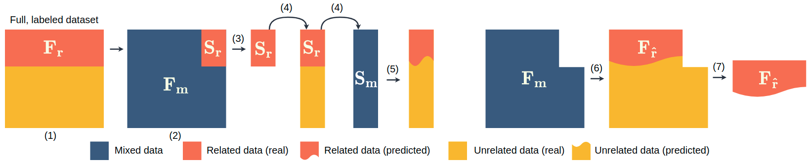
Pipeline
As showing in Figure˜7, we first construct a full dataset by randomly matching instances in MNIST and SVHN, and denote the related pairs by (full, related). We further assume access to only % of , denoted as (small, related), and denote the rest as , containing a mix of related and unrelated pairs. Next, we train a generative model on . To find a relatedness threshold, we construct a small, mixed dataset by randomly matching samples across modalities in . Given relatedness ground-truth for , we can compute the PMI for all pairs in and estimate an optimal threshold. This threshold can now be applied to the full, mixed dataset to identify related pairs giving us a new related dataset , which can be used to further improve the performance of the generative model .
Results
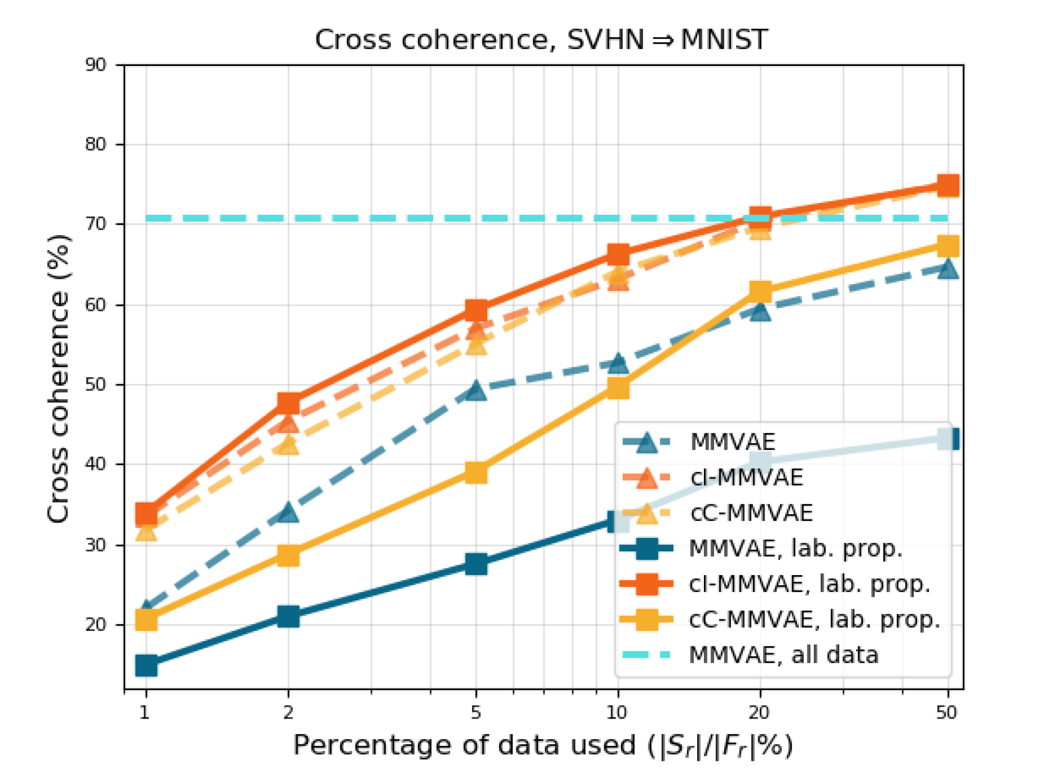
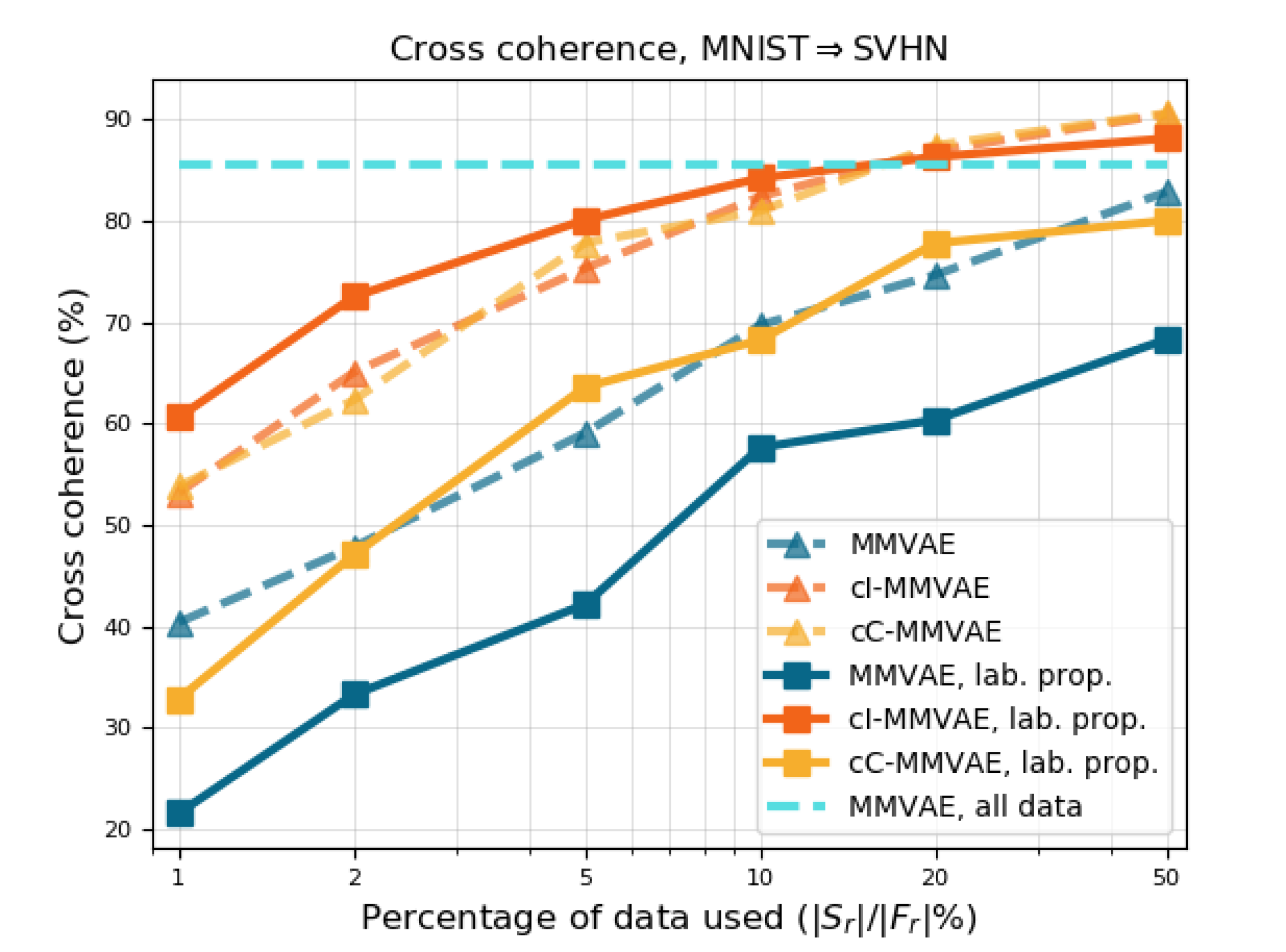
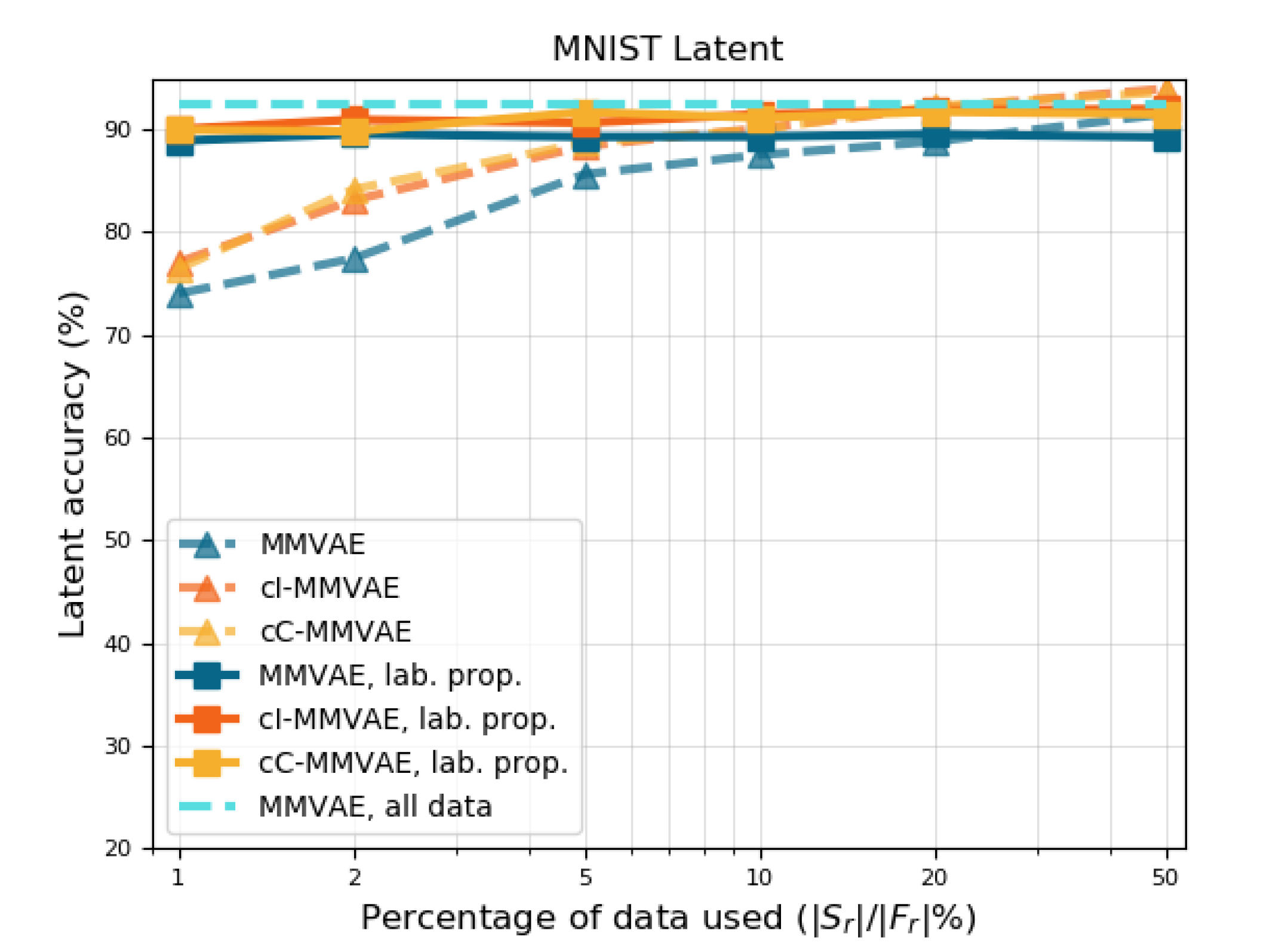
In Figure˜8 (a-e), we plot the performance of baseline MMVAE (blue) and contrastive MMVAE with IWAE (cI-MMVAE, red) and CUBO (cC-MMVAE, yellow) estimators for term of Eq Equation˜3, trained with (solid curves) and without (dotted curves) label propagation. Here, the x-axis is the proportion in size of to , i.e. the percentage of related data used to pretrain the generative model before label propagation. We compare these results to MMVAE trained on all related data (cyan horizontal line) as a “best case scenario” of these training regimes.
Clearly, label propagation using a contrastive model with IWAE estimator is helpful, and in general the improvement is greater when less data is available; Figure˜8 also shows that when is 10% of , cI-MMVAE is competitive with the performance of baseline MMVAE trained on .
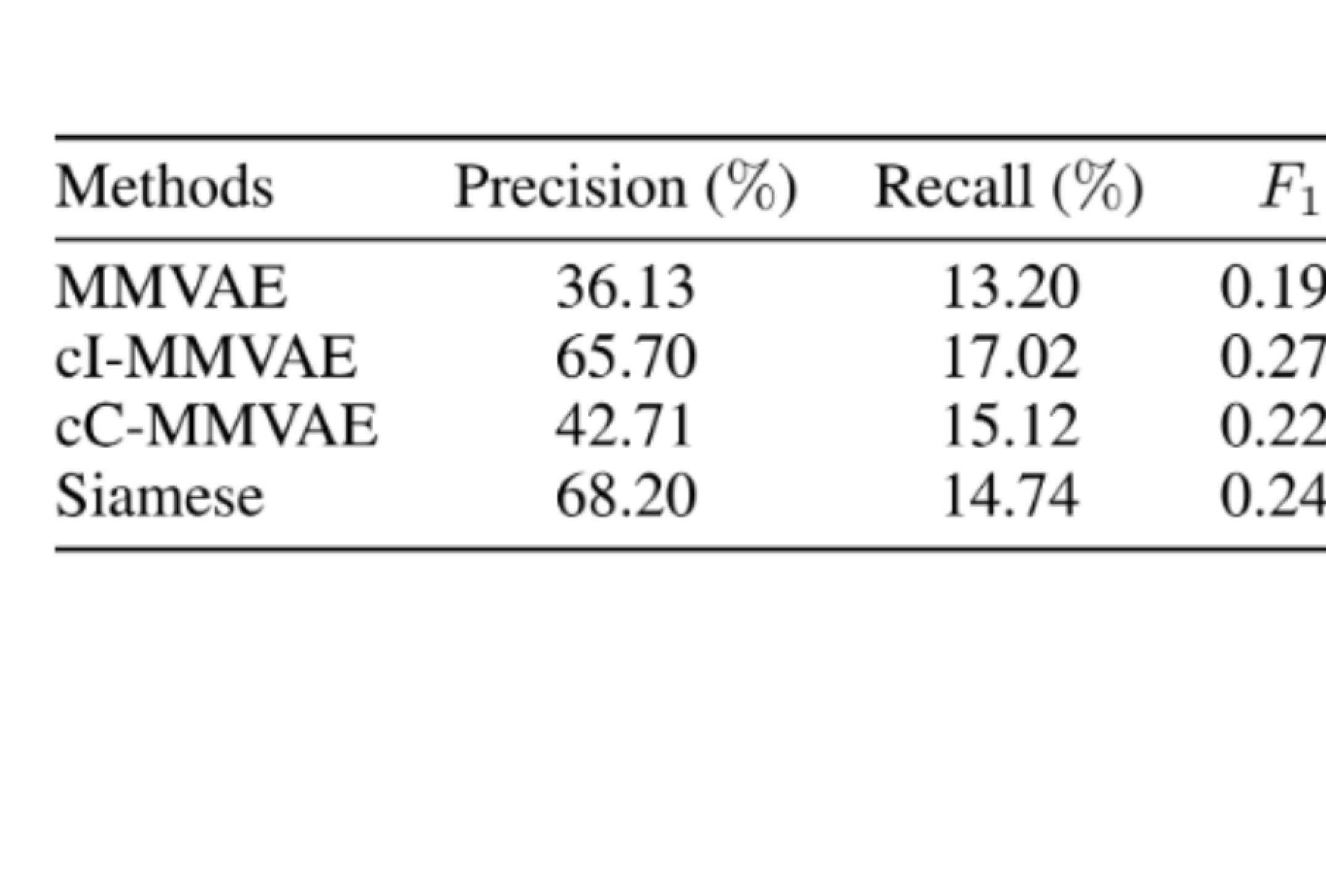
For baselines MMVAE and cC-MMVAE however, label propagation hurts performance no matter the size of , as shown by the blue and yellow curves in Figure˜8 (a-e). The advantages of cI-MMVAE is further demonstrated in Figure˜8(f), where we compute the precision, recall, and score of relatedness prediction on , for models trained on 10% of all related data. We also compare to a simple label-propagation baseline, where the relatedness of is predicted using a siamese network (Hadsell et al., 2006) trained on the same 10% dataset. Notably, while the Siamese baseline in Figure˜8(f) is a competitive predictor of relatedness, cI-MMVAE has the highest score amongst all four, making it the most reliable indicator of relatedness. Beyond that, note that with the contrastive MMVAE, relatedness can be predicted without additional training and only requires a simple threshold computation directly computed using the generative model. The fact that the cI-MMVAE’s relatedness-prediction performance is the only one that matches the Siamese baseline strongly supports the view that the contrastive loss encourages generative models to utilise and better learn the relatedness between multimodal pairs; in addition, the poor performance of cC-MMVAE shows that the advantages of having a bounded estimation to the contrastive objective by using an upper-bound for is overshadowed by the high bias of CUBO, and that one may benefit more from choosing a low variance lower-bound like IWAE.
5 Conclusion
We introduced a contrastive-style objective for multimodal VAE, aiming at reducing the amount of multimodal data needed by exploiting the distinction between "related" and "unrelated" multimodal pairs. We showed that this objective improves multimodal training, drastically reduce the amount of multimodal data needed, and establishes a strong sense of "relatedness" for the generative model. These findings hold true across a multitude of datasets, models and metrics. The positive results of our method indicates that it is beneficial to utilise the relatedness information when training on multimodal data, which has been largely ignored in previous work. While we propose to utilise it implicitly through contrastive loss, one may consider relatedness as a random variable in the graphical model and see if explicit dependency on relatedness can be useful. It is also possible to extend this idea to Generative adversarial networks (GANs), by employing an additional discriminator that evaluates relatedness between generations across modalities. We will leave these interesting directions to be explored by future work.
Acknowledgements
YS and PHST were supported by the Royal Academy of Engineering under the Research Chair and Senior Research Fellowships scheme, EPSRC/MURI grant EP/N019474/1 and FiveAI. YS was additionally supported by Remarkdip through their PhD Scholarship Programme. BP is supported by the Alan Turing Institute under the EPSRC grant EP/N510129/1. Special thanks to Elise van der Pol for helpful discussions on contrastive learning.
References
- Blum and Chawla [2001] A. Blum and S. Chawla. Learning from labeled and unlabeled data using graph mincuts. In C. E. Brodley and A. P. Danyluk, editors, Proceedings of the Eighteenth International Conference on Machine Learning (ICML 2001), Williams College, Williamstown, MA, USA, June 28 - July 1, 2001, pages 19–26. Morgan Kaufmann, 2001.
- Blum and Mitchell [1998] A. Blum and T. Mitchell. Combining labeled and unlabeled data with co-training. In Proceedings of the eleventh annual conference on Computational learning theory, pages 92–100, 1998.
- Burda et al. [2016] Y. Burda, R. B. Grosse, and R. Salakhutdinov. Importance weighted autoencoders. In Y. Bengio and Y. LeCun, editors, 4th International Conference on Learning Representations, ICLR 2016, San Juan, Puerto Rico, May 2-4, 2016, Conference Track Proceedings, 2016. URL http://arxiv.org/abs/1509.00519.
- Burkhart and Shan [2020] M. C. Burkhart and K. Shan. Deep low-density separation for semi-supervised classification. In International Conference on Computational Science, pages 297–311, 2020.
- Chen et al. [2020] T. Chen, S. Kornblith, M. Norouzi, and G. E. Hinton. A simple framework for contrastive learning of visual representations. In Proceedings of the 37th International Conference on Machine Learning, ICML 2020, 13-18 July 2020, Virtual Event, volume 119 of Proceedings of Machine Learning Research, pages 1597–1607. PMLR, 2020. URL http://proceedings.mlr.press/v119/chen20j.html.
- Dempster et al. [1977] A. P. Dempster, N. M. Laird, and D. B. Rubin. Maximum likelihood from incomplete data via the em algorithm. Journal of the royal statistical society series b-methodological, 39(1):1–22, 1977.
- Dieng et al. [2017] A. B. Dieng, D. Tran, R. Ranganath, J. W. Paisley, and D. M. Blei. Variational inference via upper bound minimization. In 31st Annual Conference on Neural Information Processing Systems, NIPS 2017, pages 2732–2741, 2017.
- Guo et al. [2019] W. Guo, J. Wang, and S. Wang. Deep multimodal representation learning: A survey. IEEE Access, 7:63373–63394, 2019.
- Hadsell et al. [2006] R. Hadsell, S. Chopra, and Y. LeCun. Dimensionality reduction by learning an invariant mapping. In 2006 IEEE Computer Society Conference on Computer Vision and Pattern Recognition (CVPR’06), volume 2, pages 1735–1742, 2006.
- He et al. [2016] K. He, X. Zhang, S. Ren, and J. Sun. Deep residual learning for image recognition. In 2016 IEEE Conference on Computer Vision and Pattern Recognition, CVPR 2016, Las Vegas, NV, USA, June 27-30, 2016, pages 770–778. IEEE Computer Society, 2016. doi: 10.1109/CVPR.2016.90. URL https://doi.org/10.1109/CVPR.2016.90.
- He et al. [2020] K. He, H. Fan, Y. Wu, S. Xie, and R. B. Girshick. Momentum contrast for unsupervised visual representation learning. In 2020 IEEE/CVF Conference on Computer Vision and Pattern Recognition, CVPR 2020, Seattle, WA, USA, June 13-19, 2020, pages 9726–9735. IEEE, 2020. doi: 10.1109/CVPR42600.2020.00975. URL https://doi.org/10.1109/CVPR42600.2020.00975.
- Hénaff [2020] O. J. Hénaff. Data-efficient image recognition with contrastive predictive coding. In Proceedings of the 37th International Conference on Machine Learning, ICML 2020, 13-18 July 2020, Virtual Event, volume 119 of Proceedings of Machine Learning Research, pages 4182–4192. PMLR, 2020. URL http://proceedings.mlr.press/v119/henaff20a.html.
- Hjelm et al. [2019] R. D. Hjelm, A. Fedorov, S. Lavoie-Marchildon, K. Grewal, P. Bachman, A. Trischler, and Y. Bengio. Learning deep representations by mutual information estimation and maximization. In 7th International Conference on Learning Representations, ICLR 2019, New Orleans, LA, USA, May 6-9, 2019. OpenReview.net, 2019. URL https://openreview.net/forum?id=Bklr3j0cKX.
- Hsu et al. [2019] C.-C. Hsu, C.-W. Lin, W.-T. Su, and G. Cheung. Sigan: Siamese generative adversarial network for identity-preserving face hallucination. IEEE Transactions on Image Processing, 28(12):6225–6236, 2019.
- Joachims [1999] T. Joachims. Transductive inference for text classification using support vector machines. In ICML ’99 Proceedings of the Sixteenth International Conference on Machine Learning, pages 200–209, 1999.
- [16] D. Massiceti, P. K. Dokania, N. Siddharth, and P. H. Torr. Visual dialogue without vision or dialogue. In NeurIPS Workshop on Critiquing and Correcting Trends in Machine Learning.
- Miller and Uyar [1996] D. J. Miller and H. S. Uyar. A mixture of experts classifier with learning based on both labelled and unlabelled data. In Advances in Neural Information Processing Systems 9, pages 571–577, 1996.
- Mnih and Kavukcuoglu [2013] A. Mnih and K. Kavukcuoglu. Learning word embeddings efficiently with noise-contrastive estimation. In C. J. C. Burges, L. Bottou, Z. Ghahramani, and K. Q. Weinberger, editors, Advances in Neural Information Processing Systems 26: 27th Annual Conference on Neural Information Processing Systems 2013. Proceedings of a meeting held December 5-8, 2013, Lake Tahoe, Nevada, United States, pages 2265–2273, 2013. URL https://proceedings.neurips.cc/paper/2013/hash/db2b4182156b2f1f817860ac9f409ad7-Abstract.html.
- Nigam et al. [2000] K. Nigam, A. K. McCallum, S. Thrun, and T. Mitchell. Text classification from labeled and unlabeled documents using em. Machine Learning, 39(2):103–134, 2000.
- Reed et al. [2016] S. E. Reed, Z. Akata, H. Lee, and B. Schiele. Learning deep representations of fine-grained visual descriptions. In 2016 IEEE Conference on Computer Vision and Pattern Recognition, CVPR 2016, Las Vegas, NV, USA, June 27-30, 2016, pages 49–58. IEEE Computer Society, 2016. doi: 10.1109/CVPR.2016.13. URL https://doi.org/10.1109/CVPR.2016.13.
- Shi et al. [2019] Y. Shi, S. Narayanaswamy, B. Paige, and P. H. S. Torr. Variational mixture-of-experts autoencoders for multi-modal deep generative models. In H. M. Wallach, H. Larochelle, A. Beygelzimer, F. d’Alché-Buc, E. B. Fox, and R. Garnett, editors, Advances in Neural Information Processing Systems 32: Annual Conference on Neural Information Processing Systems 2019, NeurIPS 2019, December 8-14, 2019, Vancouver, BC, Canada, pages 15692–15703, 2019. URL https://proceedings.neurips.cc/paper/2019/hash/0ae775a8cb3b499ad1fca944e6f5c836-Abstract.html.
- Song et al. [2016] H. O. Song, Y. Xiang, S. Jegelka, and S. Savarese. Deep metric learning via lifted structured feature embedding. In 2016 IEEE Conference on Computer Vision and Pattern Recognition, CVPR 2016, Las Vegas, NV, USA, June 27-30, 2016, pages 4004–4012. IEEE Computer Society, 2016. doi: 10.1109/CVPR.2016.434. URL https://doi.org/10.1109/CVPR.2016.434.
- [23] M. Suzuki, K. Nakayama, and Y. Matsuo. Joint multimodal learning with deep generative models. In International Conference on Learning Representations Workshop.
- Tsai et al. [2019] Y. H. Tsai, P. P. Liang, A. Zadeh, L. Morency, and R. Salakhutdinov. Learning factorized multimodal representations. In 7th International Conference on Learning Representations, ICLR 2019, New Orleans, LA, USA, May 6-9, 2019. OpenReview.net, 2019. URL https://openreview.net/forum?id=rygqqsA9KX.
- van den Oord et al. [2018] A. van den Oord, Y. Li, and O. Vinyals. Representation learning with contrastive predictive coding. arXiv preprint arXiv:1807.03748, 2018.
- Vedantam et al. [2018] R. Vedantam, I. Fischer, J. Huang, and K. Murphy. Generative models of visually grounded imagination. In 6th International Conference on Learning Representations, ICLR 2018, Vancouver, BC, Canada, April 30 - May 3, 2018, Conference Track Proceedings. OpenReview.net, 2018. URL https://openreview.net/forum?id=HkCsm6lRb.
- Wang and Isola [2020] T. Wang and P. Isola. Understanding contrastive representation learning through alignment and uniformity on the hypersphere. In Proceedings of the 37th International Conference on Machine Learning, ICML 2020, 13-18 July 2020, Virtual Event, volume 119 of Proceedings of Machine Learning Research, pages 9929–9939. PMLR, 2020. URL http://proceedings.mlr.press/v119/wang20k.html.
- Weinberger et al. [2005] K. Q. Weinberger, J. Blitzer, and L. K. Saul. Distance metric learning for large margin nearest neighbor classification. In Advances in Neural Information Processing Systems 18 [Neural Information Processing Systems, NIPS 2005, December 5-8, 2005, Vancouver, British Columbia, Canada], pages 1473–1480, 2005. URL https://proceedings.neurips.cc/paper/2005/hash/a7f592cef8b130a6967a90617db5681b-Abstract.html.
- Welinder et al. [a] P. Welinder, S. Branson, T. Mita, C. Wah, F. Schroff, S. Belongie, and P. Perona. Caltech-UCSD Birds 200. Technical Report CNS-TR-2010-001, California Institute of Technology, a.
- Welinder et al. [b] P. Welinder, S. Branson, T. Mita, C. Wah, F. Schroff, S. Belongie, and P. Perona. Caltech-UCSD Birds 200. Technical Report CNS-TR-2010-001, California Institute of Technology, b.
- Wu and Goodman [2018] M. Wu and N. D. Goodman. Multimodal generative models for scalable weakly-supervised learning. In S. Bengio, H. M. Wallach, H. Larochelle, K. Grauman, N. Cesa-Bianchi, and R. Garnett, editors, Advances in Neural Information Processing Systems 31: Annual Conference on Neural Information Processing Systems 2018, NeurIPS 2018, December 3-8, 2018, Montréal, Canada, pages 5580–5590, 2018. URL https://proceedings.neurips.cc/paper/2018/hash/1102a326d5f7c9e04fc3c89d0ede88c9-Abstract.html.
- Yildirim et al. [2018] G. Yildirim, N. Jetchev, and U. Bergmann. Unlabeled disentangling of gans with guided siamese networks. 2018.
- Yildirim [2014] I. Yildirim. From perception to conception: Learning multisensory representations. 2014.
- Zhang et al. [2020] C. Zhang, Z. Yang, X. He, and L. Deng. Multimodal intelligence: Representation learning, information fusion, and applications. IEEE Journal of Selected Topics in Signal Processing, pages 1–1, 2020.
- Zhou et al. [2003] D. Zhou, O. Bousquet, T. N. Lal, J. Weston, and B. Schölkopf. Learning with local and global consistency. In S. Thrun, L. K. Saul, and B. Schölkopf, editors, Advances in Neural Information Processing Systems 16 [Neural Information Processing Systems, NIPS 2003, December 8-13, 2003, Vancouver and Whistler, British Columbia, Canada], pages 321–328. MIT Press, 2003. URL https://proceedings.neurips.cc/paper/2003/hash/87682805257e619d49b8e0dfdc14affa-Abstract.html.
- Zhou and Li [2005] Z.-H. Zhou and M. Li. Tri-training: exploiting unlabeled data using three classifiers. IEEE Transactions on Knowledge and Data Engineering, 17(11):1529–1541, 2005.
- Zhou and Li [2010] Z.-H. Zhou and M. Li. Semi-supervised learning by disagreement. Knowledge and Information Systems, 24(3):415–439, 2010.
- Zhu et al. [2003] X. Zhu, Z. Ghahramani, and J. D. Lafferty. Semi-supervised learning using gaussian fields and harmonic functions. In T. Fawcett and N. Mishra, editors, Machine Learning, Proceedings of the Twentieth International Conference (ICML 2003), August 21-24, 2003, Washington, DC, USA, pages 912–919. AAAI Press, 2003. URL http://www.aaai.org/Library/ICML/2003/icml03-118.php.
Appendix:
Appendix A From pointwise mutual information to joint marginal likelihood
In this section, we show that for the purpose of utilising the relatedness between mutlimodal pairs, maximising the difference between pointwise mutual information between related points and unrelated points is equivalent to maximising the difference between their log joint marginal likelihoods.
To see this, we can expand as
| (41) |
In Equation˜41 the PMI difference is decomposed as two terms: the difference between joint marginal likelihoods and the difference between marginal likelihoods of different instances of -s. It is clear that since involves only one modality and only accounts for the difference in values between and , it is not relevant to the relatedness of , .
Therefore, for the purpose of utilising relatedness information, we only need to maximise through maximising term , i.e. the difference between joint marginal likelihoods.
Appendix B Connection of final objective to Pointwise Mutual Information
Here, we show that minimising the objective in Equation˜3 maximises the PMI between and :
| (42) |
We see in Equation˜42 that minimising can be decomposed to maximising both the joint marginal likelihood and an approximation of PMI . Note that since , we can be sure that the joint marginal likelihood weighting is non-negative.
Appendix C Generalisation to Modalities
In this section we show how the contrastive loss generalise to cases where number of modalities considered is greater than 2.
Given observations from modalities , where denotes unimodal dataset of modalit of size , i.e. . Similar to Equation˜1, we can write the assymetrical contrastive loss for any observation from modality , where negative samples are taken for all other modalities:
| (43) |
We can therefore rewrite Equation˜2 as:
| (44) | ||||
| (45) |
where is the number of negative samples, all are approximated by the following joint ELBO for modalities:
| (46) |
While the above gives us the true generalisation of Equation˜2, we note that the number of times where ELBO needs to be evaluated in Equation˜45 is , making it difficult to implement this objective in practice, especially on more complicated datasets. We therefore propose a simplified version of the objective, where we estimate the second term of Equation˜45 with sets of random samples from all modalities. Specifically, we can precompute the following random index matrix :
| (47) |
where each entry of is a random integer taken from range . We can then replace the second term of Equation˜45 random samples selected by the indices in , giving us
| (48) |
The number of times ELBO needs to be computed is now , and is no longer relevant to the number of modalities .
We can now also generalise the final objective in Equation˜3 to modalities:
| (49) |
Appendix D The Ineffectiveness of training with only
We demonstrate why training with the contrastive loss proposed in Equation˜2 is ineffective, and why additional ELBO term is needed for the final objective. As we show in Figure˜9, when training with only, while the contrastive loss (green) quickly drops to zero, both term and in Equation˜2 also reduces drastically. This means the joint marginal likelihood of any generation is small regardless the relatedness of .
In comparison, we also plot the training curve for model trained on the final objective in Equation˜3, which upweights term in Equation˜2 by . We see in Figure˜10 that by setting , the joint marginal likelihood (yellow and blue curve) improves during training, while (green curve) gets minimised.
Appendix E Ablation study of
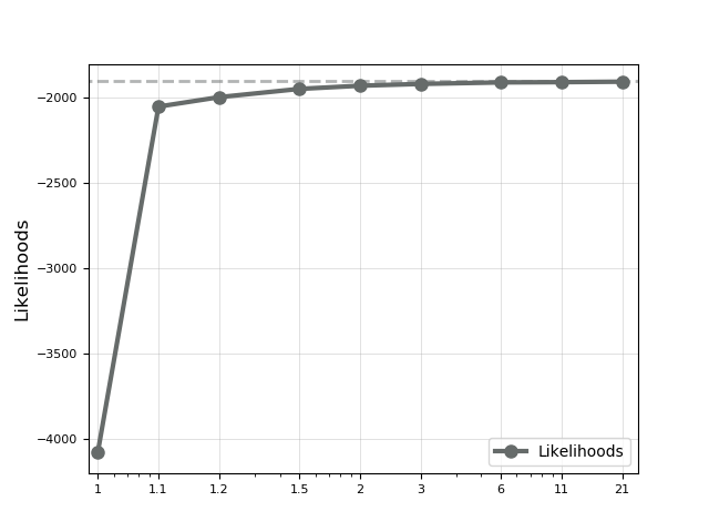
In §˜3, we specified that needs to be greater than to offset the negative effect of minimising ELBO through term in Equation˜3. Here, we study the effect of in details.
Figure˜11 compares latent accuracy, cross coherence and joint coherence of MMVAE on MNIST-SVHN dataset trained on different values of . Note that here we only consider cases where , since the minimum value of is 1. In this case, the loss reduces to the original contrastive objective in Equation˜2.
A few interesting observations from the plot are as follows: First, when , the model is trained using the contrastive loss only, and as we showed is an ineffective objective for generative model learning. This is verified again in Figure˜11 — when , both coherences and latent accuracies take on extremely low values; interestingly, there is a significant boost of performance across all metrics by simply increasing the value of from 1 to 1.1; after that, as the value of increases, performance on most metrics decreases monotonically (joint coherence being the only exception), and eventually converges to baseline MMVAE (dotted lines in Figure˜11). This is unsurprising, since the final objective in Equation˜3 reduces to the original joint ELBO as approaches infinity.
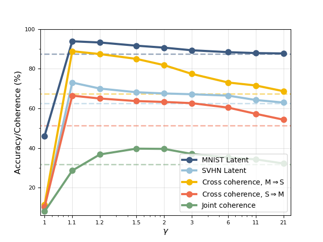
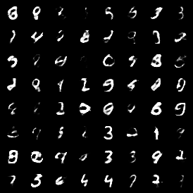
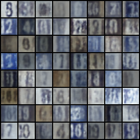
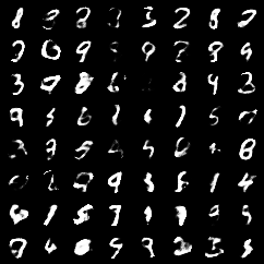
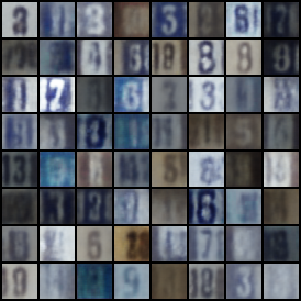
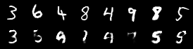
Figure˜11 seems to suggest that is the optimal value for hyperparameter , however close inspection of the qualitative generative results shows that this might not be the case. See Figure˜12 for a comparison of the model’s generation between MMVAE models trained on (from left to right) , and (i.e. original MMVAE). Although yields model with high coherence scores, we can clearly see from the left-most column of Figure˜12 that the generation of the model seems deprecated, especially for the SVHN modality, where the backgrounds of model’s generation appear to be unnaturally spotty and deformed. This problem is mitigated by increasing — as shown in Figure˜11, the image generation quality of (middle column) is not visibly different from that of (right column).
To verify this observation, we also compute the marginal log likelihood to quantify the quality of generations. We compute this for all s considered in Figure˜11, and take the average over the entire test set. From the results in Figure˜13, we can see a significant increase of the log likelihood between to . This gain in image generation quality then slows down as further increases, and as all other metrics converges to the original MMVAE model.
Appendix F Architecture
We use architectures listed in Appendix˜F for the unimodal encoder and decoder for MMVAE, MVAE and JMVAE. For JMVAE we use an extra joint encoder, the architecture of which is described in Appendix˜F.
| Encoder | Decoder |
|---|---|
| Input | Input |
| FC. 400 ReLU | FC. 400 ReLU |
| FC. , FC. | FC. 1 x 28 x 28 Sigmoid |
| Encoder | Decoder |
|---|---|
| Input | Input |
| FC. 1024 ELU | FC. 256 ELU |
| FC. 512 ELU | FC. 512 ELU |
| FC. 256 ELU | FC. 1024 ELU |
| FC. , FC. | FC. 2048 |
| Encoder |
|---|
| Input |
| Word Emb. 128 |
| 4x4 conv. 32 stride 2 pad 1 & BatchNorm2d & ReLU |
| 4x4 conv. 64 stride 2 pad 1 & BatchNorm2d & ReLU |
| 4x4 conv. 128 stride 2 pad 1 & BatchNorm2d & ReLU |
| 1x4 conv. 256 stride 1x2 pad 0x1 & BatchNorm2d & ReLU |
| 1x4 conv. 512 stride 1x2 pad 0x1 & BatchNorm2d & ReLU |
| 4x4 conv. L stride 1 pad 0, 4x4 conv. L stride 1 pad 0 |
| Decoder |
| Input |
| 4x4 upconv. 512 stride 1 pad 0 & ReLU |
| 1x4 upconv. 256 stride 1x2 pad 0x1 & BatchNorm2d & ReLU |
| 1x4 upconv. 128 stride 1x2 pad 0x1 & BatchNorm2d & ReLU |
| 4x4 upconv. 64 stride 2 pad 1 & BatchNorm2d & ReLU |
| 4x4 upconv. 32 stride 2 pad 1 & BatchNorm2d & ReLU |
| 4x4 upconv. 1 stride 2 pad 1 & ReLU |
| Word Emb.T 1590 |
| Encoder |
|---|
| Input |
| 4x4 conv. 32 stride 2 pad 1 & BatchNorm2d & ReLU |
| 4x4 conv. 64 stride 2 pad 1 & BatchNorm2d & ReLU |
| 4x4 conv. 128 stride 2 pad 1 & BatchNorm2d & ReLU |
| 1x4 conv. 256 stride 1x2 pad 0x1 & BatchNorm2d & ReLU |
| 1x4 conv. 512 stride 1x2 pad 0x1 & BatchNorm2d & ReLU |
| 4x4 conv. L stride 1 pad 0, 4x6 conv. L stride 1 pad 0 |
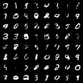
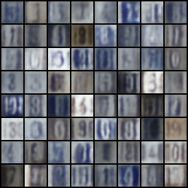
Appendix G Qualitative Results on MNIST-SVHN
G.1 Generative Results & Marginal Likelihoods on MNIST-SVHN
G.1.1 MMVAE
MMVAE cI-MMVAE cC-MMVAE
| MNIST, SVHN | MMVAE | ||||
|---|---|---|---|---|---|
| cI-MMVAE | |||||
| cC-MMVAE | |||||
| SVHN, MNIST | MMVAE | ||||
| cI-MMVAE | |||||
| cC-MMVAE |
G.1.2 MVAE
MVAE cI-MVAE cC-MVAE
| MNIST, SVHN | MVAE | ||||
|---|---|---|---|---|---|
| cI-MVAE | |||||
| cC-MVAE | |||||
| SVHN, MNIST | MVAE | ||||
| cI-MVAE | |||||
| cC-MVAE |
G.1.3 JMVAE
JMVAE cI-JMVAE cC-JMVAE
| MNIST, SVHN | JMVAE | ||
|---|---|---|---|
| cI-JMVAE | |||
| cC-JMVAE | |||
| SVHN, MNIST | JMVAE | ||
| cI-JMVAE | |||
| cC-JMVAE |
G.2 Generation diversity
To further demonstrate that the improvements from our contrastive objective did not come at a price of sacrifising generation diversity, in Figure˜17 we show histograms of the number of examples generated for each class with samples from prior. Similar to how we compute joint coherence, the class label of generated images are determined using classifiers trained on the original MNIST and SVHN dataset.
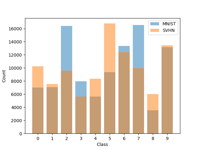
We can see that the contrastive models (cI- and cI-) are capable of generating examples from different classes, and for MMVAE and MVAE the histogram of contrastive models are more uniform than the original models (less variance between class counts).
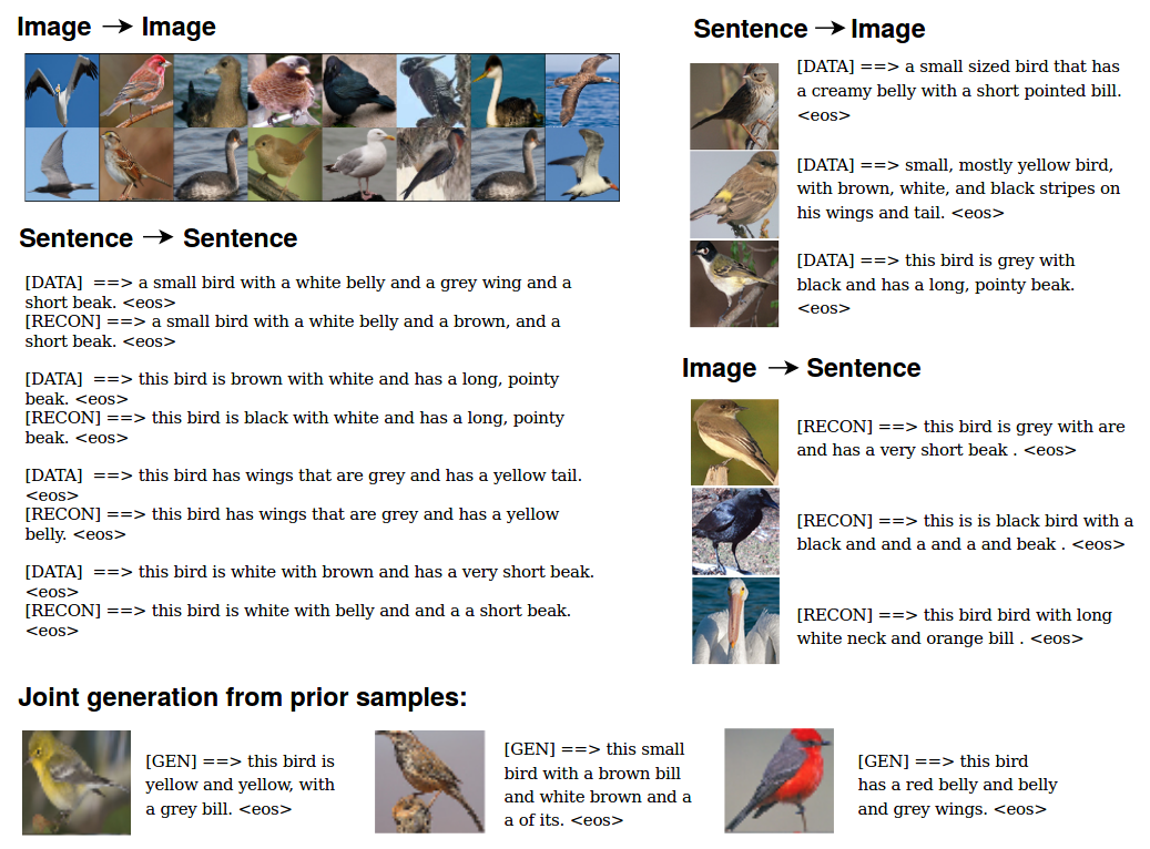
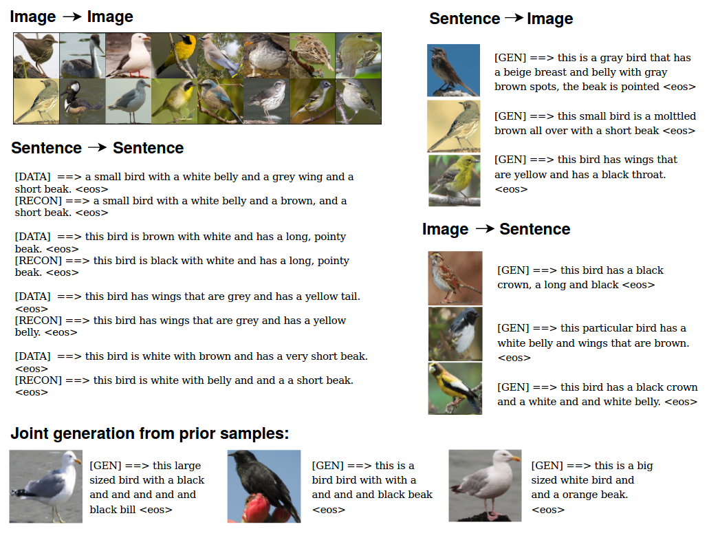
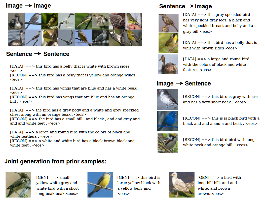
Appendix H Qualitative results on CUB
The generative results of MMVAE, cI-MMVAE and cC-MMVAE on CUB Image-Caption dataset are as shown in Figure˜18, Figure˜19 and Figure˜20. Note that for the generation in the vision modality, we reconstruct and generate features from ResNet101 and perform nearest neighbour search in all the features in train set to showcase our generation results.