Relations among Hamiltonian, area-preserving, and non-wandering flows on surfaces
Abstract.
Area-preserving flows on compact surfaces are one of the classic examples of dynamical systems, also known as multi-valued Hamiltonian flows. Though Hamiltonian, area-preserving, and non-wandering properties for flows are distinct, there are some equivalence relations among them in the low-dimensional cases. In this paper, we describe equivalence and difference for continuous flows among Hamiltonian, divergence-free, and non-wandering properties topologically. More precisely, let be a continuous flow with finitely many singular points on a compact surface. We show that is Hamiltonian if and only if is a non-wandering flow without locally dense orbits whose extended orbit space is a directed graph without directed cycles. Moreover, non-wandering, area-preserving, and divergence-free properties for are equivalent to each other.
Key words and phrases:
Flows on surfaces, non-wandering flows, area-preserving flows, divergence-free flows, Hamiltonian flows2010 Mathematics Subject Classification:
Primary 37E35; Secondary 37A05,37J05,37G301. Introduction
Area-preserving flows on compact surfaces are one of the basic and classic examples of dynamical systems, also known as locally Hamiltonian flows or equivalently multi-valued Hamiltonian flows. The measurable properties of such flows are studied from various aspects [chaika2021singularity, conze2011cocycles, forni1997solutions, frkaczek2012ergodic, forni2002deviation, kanigowski2016ratner, kulaga2012self, ravotti2017quantitative, ulcigrai2011absence]. For instance, the study of area-preserving flows for their connection with solid-state physics and pseudo-periodic topology was initiated by Novikov [novikov1982hamiltonian]. The orbits of such flows also arise in pseudo-periodic topology, as hyperplane sections of periodic manifolds (cf. [arnol1991topological, zorich1999leaves]). Moreover, any Hamiltonian flows on compact surfaces are examples of area-preserving flows. The difference between Hamiltonian and area-preserving flows on closed surfaces can be represented by harmonic flows, which are generated by the dual vector fields of harmonic one-forms. The topological invariants of Hamiltonian flows with finitely many singular points on compact surfaces are constructed from integrable systems points and dynamical systems points of views, and the structural stability are characterized [bolsinov1999exact, Nikolaenko20, Oshemkov10, sakajo2015transitions, sakajo2018tree, yokoyama2013word]. On the other hand, any area-preserving flows are non-wandering flows. Non-wandering flow on surfaces are classified and decomposed into elementary cells under finite existence of singular points, and are topologically characterized, and the topological invariants are constructed [cobo2010flows, nikolaev1998finite, nikolaev2001non, yokoyama2016topological, yokoyama2017decompositions, yokoyama2017genericity].
In this paper, we describe equivalence and difference for continuous flows on compact surfaces among Hamiltonian, divergence-free, and non-wandering properties. To state precisely, recall some concepts. By a flow, we mean a continuous -action. A flow is non-wandering if any points are non-wandering. A flow on a surface is Hamiltonian (resp. area-preserving, divergence-free) if it is topologically equivalent to the flow generated by a smooth Hamiltonian (resp. area-preserving, divergence-free) vector field. Notice that each of the Hamiltonian, area-preserving, divergence-free properties is not preserved by topological equivalence for vector fields but is preserved by one for flows. We consider the following question.
Question 1.
Is there a difference between area-preserving flows and non-wandering flows on compact surfaces?
We answer negatively under the finite existence of singular points. In other words, we have the following equivalence among non-wandering, area-preserving, and divergence-free flows.
Theorem A.
The following are equivalent for a flow with finitely many singular points on a compact surface:
(1) The flow is is non-wandering.
(2) The flow is is area-preserving.
(3) The flow is is divergence-free.
We also ask the following similar question, which is posed by M. Asaoka [asaoka2016] and is a motivative question of Question 1.
Question 2.
What is a difference between Hamiltonian flows and non-wandering flows on surfaces?
To answer this question, we characterize a Hamiltonian flow under the finite existence of singular points as follows.
Theorem B.
The following are equivalent for a flow with finitely many singular points on an orientable compact surface :
(1) The flow is Hamiltonian.
(2) The flow is non-wandering, there are no locally dense orbits, and the extended orbit space is a directed graph without directed cycles.
Here the extended orbit space is a quotient space defined by if either and are contained a multi-saddle connection or there is an orbit which contains and but is not contained in any multi-saddle connections. The non-existence of directed cycles can not be replaced by the non-existence of closed transversals in the previous theorem (see the third example as in Figure 7 in §5). On the sphere, there is no difference between Hamiltonian flows and non-wandering flows under the finite existence of singular points as follows.
Corollary C.
Let be a flow with finitely many singular points on a compact surface contained in a sphere.
The following statements are equivalent:
The flow is non-wandering.
The flow is area-preserving.
The flow is divergence-free.
The flow is Hamiltonian.
The present paper consists of five sections. In the next section, as preliminaries, we introduce fundamental concepts. In §3, we characterize a Hamiltonian flow with finitely many singular points on a compact surface. In §4, we show the equivalence among non-wandering flows, area-preserving flows, and divergence-free flows on compact surfaces under the finite existence of singular points. In the final section, examples of non-Hamiltonian area-preserving flows are described.
2. Preliminaries
2.1. Notion of topology
Denote by the closure of a subset of a topological space, by the interior of , and by the boundary of , where is used instead of the set difference when . We define the border by of . A boundary component of a subset is a connected component of the boundary of . A subset is locally dense if its closure has a nonempty interior. A boundary component of a subset is a connected component of the boundary of . By a surface, we mean a two dimensional paracompact manifold, that does not need to be orientable.
2.1.1. Directed topological graphs
A directed topological graph is a topological realization of a 1-dimensional simplicial complex with a directed structure on edges. A directed cycle in a directed topological graph is an embedded cycle whose edges are oriented in the same direction.
2.1.2. Curves and arc
A curve is a continuous mapping where is a non-degenerate connected subset of a circle . A curve is simple if it is injective. We also denote by the image of a curve . Denote by the boundary of a curve , where is the boundary of . Put . A simple curve is a simple closed curve if its domain is (i.e. ). An arc is a simple curve whose domain is a non-degenerate interval.
2.1.3. Reeb graph of a function on a topological space
For a function on a topological space , the Reeb graph of a function on a topological space is a quotient space defined by if there are a number and a connected component of which contains and .
2.2. Notion of dynamical systems
We recall some basic notions. A good reference for most of what we describe is a book by S. Aranson, G. Belitsky, and E. Zhuzhoma [aranson1996introduction].
By a flow, we mean a continuous -action on a surface. Let be a flow on a compact surface . Then is a homeomorphism on . For , define by . For a point of , we denote by the orbit of (i.e. ). An orbit arc is a non-degenerate arc contained in an orbit. A subset of is said to be invariant (or saturated) if it is a union of orbits. The saturation of a subset is the union of orbits intersecting . A point of is singular if for any and is periodic if there is a positive number such that and for any . A point is closed if it is either singular or periodic. Denote by (resp. ) the set of singular (resp. periodic) points. A point is wandering if there are its neighborhood and a positive number such that for any . Then such a neighborhood is called a wandering domain. A point is non-wandering if it is not wandering (i.e. for any its neighborhood and for any positive number , there is a number with such that ).
For a point , define the -limit set and the -limit set of as follows: , . For an orbit , define and for some point . Note that an -limit (resp. -limit) set of an orbit is independent of the choice of a point in the orbit. A separatrix is a non-singular orbit whose -limit or -limit set is a singular point.
A point of is Poisson stable (or strongly recurrent) if . A point of is recurrent if . An orbit is singular (resp. periodic, closed, non-wandering, recurrent, Poisson stable) if it consists of singular (resp. periodic, closed, non-wandering, recurrent, Poisson stable) points. A flow is non-wandering (resp. recurrent) if each point is non-wandering (resp. recurrent). A quasi-minimal set is an orbit closure of a non-closed recurrent orbit. The closure of a non-closed recurrent orbit is called a Q-set.
2.2.1. Orbit classes and quotient spaces of flows
The (orbit) class of an orbit is the union of orbits each of whose orbit closure corresponds to (i.e. ). For a flow on a topological space , the orbit space (resp. orbit class space ) of an invariant subset of is a quotient space defined by if (resp. ). Notice that an orbit space is the set as a set. Moreover, the orbit class space is the set with the quotient topology.
2.2.2. Topological properties of orbits
An orbit is proper if it is embedded, locally dense if its closure has a nonempty interior, and exceptional if it is neither proper nor locally dense. A point is proper (resp. locally dense, exceptional) if its orbit is proper (resp. locally dense, exceptional). Denote by (resp. , ) the union of locally dense orbits (resp. exceptional orbits, non-closed proper orbits). Note that an orbit on a paracompact manifold (e.g. a surface) is proper if and only if it has a neighborhood in which the orbit is closed [yokoyama2019properness]. This implies that a non-recurrent point is proper and so that a non-proper point is recurrent. In [cherry1937topological, Theorem VI], Cherry showed that the closure of a non-closed recurrent orbit of a flow on a manifold contains uncountably many non-closed recurrent orbits whose closures are . This means that each non-closed recurrent orbit of a flow on a manifold has no neighborhood in which the orbit is closed, and so is not proper. In particular, a non-closed proper orbit is non-recurrent. Therefore the union of non-closed proper orbits is the set of non-recurrent points and that , where denotes a disjoint union. Hence we have a decomposition .
2.2.3. Types of singular points
A point is a center if for any its neighborhood , there is an invariant open neighborhood of such that is an open annulus which consists of periodic orbits as in the left on Figure 1, where is used instead of when . A --saddle (resp. -saddle) is an isolated singular point on (resp. outside of) with exactly -separatrices, counted with multiplicity as in Figure 1.
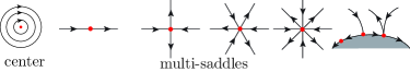
A multi-saddle is a -saddle or a --saddle for some . A -saddle is topologically an ordinary saddle and a --saddle is topologically a -saddle.
2.2.4. Multi-saddle connection diagrams
The multi-saddle connection diagram is the union of multi-saddles and separatrices between multi-saddles. A multi-saddle connection is a connected component of the multi-saddle connection diagram. Note that a multi-saddle connection is also called a poly-cycle.
2.2.5. Flow boxes, periodic annuli, transverse annuli, and periodic invariant subsets
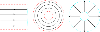
A subset is a flow box if there are bounded non-degenerate intervals and a homeomorphism such that the image for any is an orbit arc as in the left on Figure 2, a open (resp. closed) periodic annulus is an open (resp. closed) annulus consisting of periodic orbits as in the middle on Figure 2, and an open (resp. closed) transverse annulus is an open (resp. closed) annulus contained as in the right on Figure 2.
A periodic torus (resp. Klein bottle, Möbius band) is a torus (resp. Klein bottle, Möbius band) consisting of periodic orbits. Pasting one center (resp. two centers) with boundary components of an open periodic annulus, we obtain an open center disk (resp. rotating sphere). Pasting one center with the boundary of an open periodic Möbius band, we obtain a rotating projective plane. In other words, a rotating sphere (resp. projective plane) is a flow on a sphere (resp. projective plane) that consists of two centers (resp. one center) and periodic orbits. An open (resp. closed) center disk is a flow on an open (resp. closed) disk that consists of a center and periodic orbits.
2.3. Characterizations of non-wandering flows
Recall a following characterization of non-wandering flow which is essentially based on [yokoyama2016topological, Theorem 2.5].
Lemma 2.1.
Let be a flow on a compact surface .
The following statements are equivalent:
The flow is non-wandering.
.
.
.
In any case, we have .
Proof.
Recall that and that the union is the set of points which are not recurrent. By the Maǐer theorem [mayer1943trajectories, markley1970number], the closure is a finite union of closures of exceptional orbits and so is nowhere dense. By [yokoyama2016topological, Lemma 2.3], the union is a neighborhood of . This means that if . Therefore conditions , , and are equivalent. By [yokoyama2016topological, Theorem 2.5], conditions and are equivalent. Suppose that is non-wandering. [yokoyama2016topological, Proposition 2.6] implies . ∎
2.4. Fundamental notion related to Hamiltonian flows on a compact surface
A vector field for any on an orientable surface is Hamiltonian if there is a function such that as a one-form, where is a volume form of . In other words, locally the Hamiltonian vector field is defined by for any local coordinate system of a point . A flow is Hamiltonian if it is topologically equivalent to a flow generated by a smooth Hamiltonian vector field. Note that a volume form on an orientable surface is a symplectic form. It is known that a () Hamiltonian vector field on a compact surface is structurally stable with respect to the set of Hamiltonian vector fields if and only if both each singular point is non-degenerate and each separatrix of a saddle is homoclinic, and each separatrix on a -saddle connects a boundary component (see [ma2005geometric, Theorem 2.3.8, p. 74]).
By [cobo2010flows, Theorem 3], any singular points of a Hamiltonian vector field with finitely many singular points on a compact surface is either a center or a multi-saddle, and the Reeb graph of the Hamiltonian generating is a directed topological graph which is also a quotient space of the orbit space of the generating flow. In other words, the Reeb graph is obtained from the orbit space by collapsing multi-saddle connections into singletons. Note that the orbit space of a Hamiltonian flow is not a directed topological graph.
In the analogy of the collapse, we define the extended orbit to describe “reduced” orbit spaces as follows. By an extended orbit of a flow, we mean a multi-saddle connection or an orbit that is not contained in any multi-saddle connection. Denote by the extended orbit containing . The quotient space by extended orbits of a flow on a surface is called the extended orbit space and denoted by .
2.4.1. Divergence-free flows, area-preserving flows, and multi-valued Hamiltonians
A vector field for any on a surface with a Riemannian metric is area-preserving if the area form is preserved under pullback (i.e. ) by homeomorphisms for any , where is the flow generated by . A vector field for any is divergence-free if , where . We call that a flow is area-preserving (resp. divergence-free) if it is topologically equivalent to a flow generated by a smooth area-preserving (resp. divergence-free) vector field. Note that the divergence can be also determined by a condition where is the Lie derivative along . Liouville’s theorem implies the following observation.
Lemma 2.2.
A flow on a surface is area-preserving if and only if it is a divergence-free.
Proof.
Let be the flow generated by a smooth vector field on a surface. Since , we have that for any if only if . ∎
A flow generated by a vector field on a surface is a multi-valued Hamiltonian flow if there are finitely many pairs of charts with and smooth Hamiltonians on the charts such that the flow is a solution to the equations and (i.e. ). Then is called a multi-valued Hamiltonian on .
3. Characterization of Hamiltonian surface flows with finitely many singular points on compact surfaces
Let be a flow on a compact connected surface . We have the following characterization of a non-wandering flow with finitely many singular points but without locally dense orbits.
Lemma 3.1.
The following statements are equivalent for a flow with finitely many singular points but without locally dense orbits on a compact connected surface :
The flow is non-wandering.
Each connected component of the complement is either a rotating sphere, an open center disk, an open periodic annulus, a periodic torus, a periodic Klein bottle, a rotating projective plane, or a periodic Möbius band.
In any case, , the multi-saddle connection diagram consists of finitely many orbits, and the extended orbit space is a finite directed topological graph.
Proof.
Condition (2) implies that and so that is non-wandering. Conversely, suppose that is non-wandering. By [yokoyama2016topological, Corollary 2.9], the periodic point set is open. From Lemma 2.1, we have . [cobo2010flows, Theorem 3] implies that each singular point of a non-wandering flow with finitely many singular points on a compact surface is either a center or a multi-saddle. The finite existence of multi-saddle implies that the multi-saddle connection diagram consists of finitely many orbits. Then . The union defined in [yokoyama2017decompositions] is the union of singular points and separatrices between multi-saddles. This means that is the union of centers and the multi-saddle connection diagram . [yokoyama2017decompositions, Theorem A] (or [katok1997introduction, nikolaev1999flows] or [nikolaev2001non, Proposition 2]) implies that each connected component of is either a periodic annulus, a periodic torus, a periodic Klein bottle, or a periodic Möbius band. Adding centers, each connected component of is either a rotating sphere, an open center disk, an open periodic annulus, a periodic torus, a periodic Klein bottle, a rotating projective plane, or a periodic Möbius band. For any connected component of , the restriction is an interval. Since any multi-saddle connections are singletons in , the extended orbit space is a finite directed topological graph. From , we have . This means that is non-wandering. ∎
We show that non-wandering flows with finitely many singular points are divergence-free.
Lemma 3.2.
Let be a flow with finitely many singular points on a compact connected surface .
The following statements are equivalent:
The flow is a non-wandering flow without locally dense orbits.
The flow is a divergence-free flow without locally dense orbits.
Moreover, if is orientable and the extended orbit space has no directed cycle as a directed graph, then the following condition is equivalent to one of the above conditions:
The flow is Hamiltonian.
Proof.
We may assume that is connected. Since Hamiltonian vector fields are divergence-free and the existence of a Hamiltonian implies the non-existence of locally dense orbits, condition implies condition . Suppose that is a divergence-free flow without locally dense orbits. Since any divergence-free vector fields on compact surfaces have no wandering domains, the flow is non-wandering. This means that condition implies condition .
Conversely, suppose that is a non-wandering flow without locally dense orbits. Then there are no limit circuits. From Lemma 3.1, we have that and that each singular point of is either a center or a multi-saddle. Notice that if is orientable and has no directed cycle as a directed graph, then multi-valued Hamiltonians can be chosen as single-valued Hamiltonians.
Suppose that . Then is topologically equivalent to a flow given by multi-valued Hamiltonians. Since multi-valued Hamiltonian vector fields are divergence-free, the given flow is a flow generated by a divergence-free vector field. This means that the flow is divergence-free. If is orientable and has no directed cycle as a directed graph then is Hamiltonian.
Suppose that . We may assume that there are singular points. The non-existence of non-recurrent points implies that any singular points are centers. Then is axisymmetric rotating on either a sphere, a closed disk, or a projective plane and so is topologically equivalent to a flow given by multi-valued Hamiltonians. This means that the flow is divergence-free. As above, if is orientable and has no directed cycle as a directed graph, then is Hamiltonian.
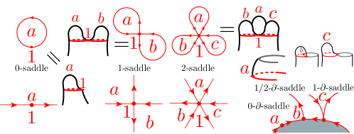
Thus we may assume that . Then is not pointwise periodic and so . Lemma 3.1 implies that the complement of the multi-saddle connection diagram consists of periodic annuli, open center disks, open Möbius bands each of whose orbit spaces is homeomorphic to an interval . Since -saddle (resp. --saddle) can be realized by a Hamiltonian with (resp.) centers as Figure 3, any flow restricted to a small simply connected open neighborhood of a multi-saddle is topologically equivalent to a flow generated by a smooth Hamiltonian vector field.
Since there are trivial flow boxes along separatrices between multi-saddles, we can extend such a flow given by Hamiltonians near multi-saddles into a flow given by multi-valued Hamiltonians near the multi-saddle connection diagram. We can take such that is homotopic to the union and so the complement is a disjoint union of invariant closed periodic annuli, invariant closed center disks, and invariant closed Möbius bands each of whose orbit spaces is homeomorphic to a closed interval. Since the restrictions of into these connected components of are topologically equivalent to flows generated by multi-valued Hamiltonian vector fields, we can construct a flow given by multi-valued Hamiltonians. This means that the flow is divergence-free. As above, if is orientable and has no directed cycle as a directed graph, then is Hamiltonian. ∎
The previous theorem implies an answer, which is Theorem B, for a question when a non-wandering flow with finitely many singular points on an orientable compact connected surface becomes Hamiltonian as follows.
3.1. Proof of Theorem B
Suppose that is Hamiltonian. Let be the Hamiltonian of and . Then there is a quotient map with . This means that there are no directed cycles in . Lemma 3.2 implies the converse.
4. Correspondence of non-wandering flows and divergence-free flows on compact surfaces under finiteness of singular points
Recall the following fact.
Lemma 4.1.
Let be a flow on a compact surface. For any locally dense orbit, there is a closed transverse intersecting it.
For self-containedness, we state the following proof.
Proof.
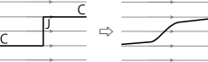
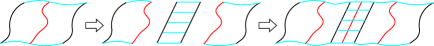
Fix a locally dense orbit . Let be a closed orbit arc in from to and a closed transverse arc with . If the first return map on is orientable near along , then apply the waterfall construction to the simple closed curve (see Figure 4), and so we have a closed transversal which intersects and is near .
Thus we may assume that the first return map on is not orientable near . Take a closed orbit arc from to with . Let be the sub-arc in and the sub-arc in such that and . If the return map on is orientable near along , then the waterfall construction to the simple closed curve implies a closed transversal that intersects and is near . If the return map on is not orientable near along , then the waterfall construction to the simple closed curve implies a closed transversal which intersects and is near . ∎
Recall that a periodic orbit is one-sided if it is either a boundary component of a surface or has a small neighborhood which is a Möbius band.
4.1. Proof of Theorem A
Let be a flow with finitely many singular points on a compact connected surface . Lemma 2.2 implies the equivalence between area-preserving property and divergence-free property for . Suppose that is divergence-free. [cobo2010flows, Theorem 3] implies that each singular point is either a center or a multi-saddle. Since any divergence-free vector fields on compact surfaces have no wandering domains, the flow is non-wandering.
Conversely, suppose that is non-wandering. Lemma 2.1 implies the non-existence of exceptional orbits of . The smoothing theorem [gutierrez1986smoothing] implies that is topologically equivalent to a -flow. It is known that a total number of Q-sets for cannot exceed if is an orientable surface of genus [mayer1943trajectories], and if is a non-orientable surface of genus [markley1970number] (cf. Remark 2 [aranson1996maier]). There are finitely many distinct Q-sets. By induction of the number of Q-sets, we will show the assertion. If there are no Q-sets, then Lemma 3.2 implies that is divergence-free. Suppose that there are Q-sets. Fix a Q-set . [cherry1937topological, Theorem VI] implies that contains infinitely many Poisson stable orbits. Fix a Poisson stable orbit in . By Lemma 4.1, there is a closed transversal intersecting . Then . Let be a smooth vector field whose generating flow is topological equivalent to .
We claim that the first return map of is topologically conjugate to a minimal interval exchange transformation on the circle . Indeed, by the structure theorem of Gutierrez [gutierrez1986smoothing] (see also [gutierrez1986smoothing, Lemma 3.9] and [nikolaev1999flows, Theorem 2.5.1]), for the closed transversal for the Q-set , the first return map is well-defined and topologically semi-conjugate to a minimal interval exchange transformation . Since is locally dense and contains , the first return map is topologically conjugate to the minimal interval exchange transformation .
Therefore we may assume that the first return map by is a minimal interval exchange transformation. Fix an interval exchange transformation such that has periodic orbits. Denote by the intervals of interval exchange transformation . Let be the length of with . Fix an open transverse annulus which is a neighborhood of and contains no singular points. Then we also may assume that the restriction of to can be identified with a vector field on by a homeomorphism. Consider a smooth divergence-free vector field on which depends only on and which is a periodic annulus such that the first return map on by the flow generated by the resulting vector field is topological equivalent to the interval exchange transformation . Then has a periodic orbit intersecting and . Fix the corresponding periodic orbit of intersecting . Denote by the intervals of corresponding to . Then the saturations of any intervals of are invariant open periodic annuli or Möbius bands . Since any interval exchange transformation preserves the Lebesgue measure and so non-wandering, the flow generated by is non-wandering. By the inductive hypothesis, the flow is divergence-free. By construction, . Fix a divergence-free vector field whose generating flow is topologically equivalent to and a closed transversal with respect to which corresponds to . Then the first return map is topologically conjugate to . If is an open Möbius band, then the orbit space for the flow generated by is homeomorphic to a half open interval such that the periodic orbit corresponding to is one-sided and denote by . Denote by be the differences of the values the boundary components of the open invariant annulus with respect to the multi-valued Hamiltonians if is an annulus, and by the twice of the differences of the values the boundary components of the open invariant annulus with respect to the multi-valued Hamiltonians . Put . Write if is an annulus, and if is Möbius band.
We claim that we may assume that by deformations. Indeed, by the topological equivalence between and , the saturations of any intervals of the interval exchange transformation are also invariant open periodic annuli . Identify annuli with an embedded annuli of . Let be an invariant open annulus with and the connected components of . Then the set difference is a disjoint union of two invariant annuli. Removing , taking translation of with respect to the heights of , and interpolating between and as in Figure 5, the resulting annuli have the arbitrarily differences of the values the boundary components of with respect to the height.

Therefore we can choose the differences of the values the boundary components of such that . Since the constructions preserve topological equivalence, the claim is completed.
We claim that we may assume that there are a closed transversal with and an open annular neighborhood of which can be isometrically embedded into such that and that for some positive number , by deformation. Indeed, fix a small open annular neighborhood of which is a closed transverse annulus such that . For a point , denote by the orbit arc in containing . Identify with , where is a function defined by . Cutting along the closed transversal , inserting a closed annulus into the resulting two closed annuli and , and interpolate between and and between and as in Figure 6, we can obtain the resulting annuli .
Then is a closed transversal. This completes the claim.
By construction, there is a divergence-free vector field whose support is contained in and that any non-singular orbit is a periodic orbit of form and is depended only on the -coordinate in . Multiplying by a scalar if necessary, we may assume that the first return map on by is topological conjugate to and so to . This means that the flow generated by is topological equivalent to . Recall that, for any divergence-free vector field , a vector field is divergence-free if and only if so is the sum . This implies that the vector field is divergence-free and so is the flow .
4.2. Proof of Corollary C
5. Examples of non-Hamiltonian area-preserving flows
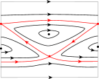
Irrational rotations on a torus are non-Hamiltonian area-preserving flows. Any flows on a torus consisting of periodic orbits are non-Hamiltonian area-preserving flows. The following example is a non-Hamiltonian area-preserving flow without closed transversals, which M. Asaoka suggested to show the necessity of the non-existence of directed cycles in Theorem B. Indeed, there is a smooth non-Hamiltonian area-preserving flow with non-degenerate singular points but without neither locally dense orbits nor closed transversals on a torus as in Figure 7.
Acknowledgement: The author would like to thank Masashi Asaoka for his motivative question and helpful comments.