Relative Reshetikhin-Turaev invariants, hyperbolic cone metrics and discrete Fourier transforms II

Ka Ho Wong and Tian Yang

Abstract

We prove the Volume Conjecture for the relative Reshetikhin-Turaev invariants proposed in [29] for all pairs $(M,K)$ such that $M{\smallsetminus}K$ is homeomorphic to the complement of the figure- $8$ knot in $S^{3}$ with almost all possible cone angles.

1 Introduction

In the first paper [29] of this series, we proposed the Volume Conjecture for the relative Reshetikhin-Turaev invariants of a closed oriented $3$ -manifold with a colored framed link inside it whose asymptotic behavior is related to the volume and the Chern-Simons invariant of the hyperbolic cone metric on the manifold with singular locus the link and cone angles determined by the coloring.

Conjecture 1.1 ([29]).

Let $M$ be a closed oriented $3$ -manifold and let $L$ be a framed hyperbolic link in $M$ with $n$ components. For an odd integer $r\geqslant 3,$ let $\mathbf{m}=(m_{1},\dots,m_{n})$ and let $\mathrm{RT}_{r}(M,L,\mathbf{m})$ be the $r$ -th relative Reshetikhin-Turaev invariant of $M$ with $L$ colored by $\mathbf{m}$ and evaluated at the root of unity $q=e^{\frac{2\pi\sqrt{-1}}{r}}.$ For a sequence $\mathbf{m}^{(r)}=(m^{(r)}_{1},\dots,m^{(r)}_{n}),$ let

\theta_{k}=\bigg{|}2\pi-\lim_{r\to\infty}\frac{4\pi m^{(r)}_{k}}{r}\bigg{|}

and let $\theta=(\theta_{1},\dots,\theta_{n}).$ If $M_{L_{\theta}}$ is a hyperbolic cone manifold consisting of $M$ and a hyperbolic cone metric on $M$ with singular locus $L$ and cone angles $\theta,$ then

\lim_{r\to\infty}\frac{4\pi}{r}\log\mathrm{RT}_{r}(M,L,\mathbf{m}^{(r)})=\mathrm{Vol}(M_{L_{\theta}})+\sqrt{-1}\mathrm{CS}(M_{L_{\theta}})\quad\quad\text{mod }\sqrt{-1}\pi^{2}\mathbb{Z},

where $r$ varies over all positive odd integers.

In the same paper [29], we also proved Conjecture 1.1 in the case that the ambient $3$ -manifold is obtained by doing an integral surgery along some components of a fundamental shadow link and the complement of the link in the ambient manifold is homeomorphic to the fundamental shadow link complement, for sufficiently small cone angles. A result of Costantino and Thurston shows that all the closed oriented $3$ -manifolds can be obtained by doing an integral Dehn filling along a suitable fundamental shadow link complement. On the other hand, it is expected that hyperbolic cone metrics interpolate the complete cusped hyperbolic metric on the $3$ -manifold with toroidal boundary and the smooth hyperbolic metric on the Dehn-filled $3$ -manifold, corresponding to the colors running from $\frac{r-1}{2}$ to $0$ or $r-2.$ Therefore, if one can push the cone angles in Theorem 1.2 from sufficiently small all the way up to $2\pi,$ then one proves the Volume Conjecture for the Reshetikhin-Turaev invariants of closed oriented hyperbolic $3$ -manifolds proposed by Chen and the second author [4]. This thus suggests a possible approach of solving Chen-Yang’s Volume Conjecture.

The main result of this paper proves Conjecture 1.1 for all pairs $(M,K)$ such that $M{\smallsetminus}K$ is homeomorphic to the figure- $8$ knot complement in $S^{3}$ with almost all possible cone angles, showing the plausibility of this new approach.

Theorem 1.2.

Conjecture 1.1 is true for all pairs $(M,L)$ such that $M{\smallsetminus}K$ is homeomorphic to the figure- $8$ knot complement $S^{3}{\smallsetminus}K_{4_{1}}$ and for all cone angles $\theta$ such that

\mathrm{Vol}(M_{K_{\theta}})>\frac{\mathrm{Vol}(S^{3}{\smallsetminus}K_{4_{1}})}{2}.

We note that if $M{\smallsetminus}K$ is homeomorphic to $S^{3}{\smallsetminus}K_{4_{1}},$ then $M$ is obtained from $S^{3}$ by doing a $\frac{p}{q}$ -surgery along $K_{4_{1}}.$ In Proposition 7.9, we show that if $(p,q)\neq(\pm 1,0),$ $(0,\pm 1),$ $(\pm 1,\pm 1),$ $(\pm 2,\pm 1),$ $(\pm 3,\pm 1),$ $(\pm 4,\pm 1)$ and $(\pm 5,\pm 1),$ then any $\theta$ less than or equal to $2\pi$ satisfies the condition of Theorem 1.2; and if $(p,q)$ is one of those sporadic cases except $(\pm 1,0),$ then any $\theta$ less than or equal to $\pi$ satisfies the condition of Theorem 1.2.

Outline of the proof. The proof follows the guideline of Ohtsuki’s method. In Proposition 3.1, we compute the relative Reshetikhin-Turaev invariants of $(M,K)$ and write them as a sum of values of holomorphic functions $f^{\pm}_{r}$ at integral points. The functions $f^{\pm}_{r}$ comes from Faddeev’s quantum dilogarithm function. Using Poisson summation formula, we in Proposition 4.1 write the invariants as a sum of the Fourier coefficients of $f_{r},$ and in Propositions 5.4, 5.5 and 5.7 we simplify those Fourier coefficients by doing some preliminary estimate. In Proposition 6.3 we show that the critical value of the functions in the two leading Fourier coefficients $\hat{f}^{\pm}_{r}(0,\dots,0)$ have real part the volume and imaginary part the Chern-Simons invariant of $M_{K_{\theta}}.$ The key observation is Lemma 6.1 that the system of critical point equations is equivalent to the system of hyperbolic gluing equations (consisting of an edge equation and a $\frac{p}{q}$ Dehn-filling equation with cone angle $\theta$ ) for a particular ideal triangulation of the figure- $8$ knot complement. In Section 7.1 we verify the conditions for the saddle point approximation showing that the growth rate of the leading Fourier coefficients are the critical values; and in Section 7.2, we estimate the other Fourier coefficients showing that they are neglectable.

Acknowledgments. The authors would like to thank Feng Luo and Hongbin Sun for helpful discussions. The second author is partially supported by NSF Grant DMS-1812008.

2 Preliminaries

For the readers’ convenience, we recall the relative Reshetikhin-Turaev invariants, hyperbolic cone metrics and the classical and quantum dilogarithm functions respectively in Sections 2.1, 2.2, 2.3 and 2.4.

2.1 Relative Reshetikhin-Turaev invariants

In this article we will follow the skein theoretical approach of the relative Reshetikhin-Turaev invariants [2, 18] and focus on the root of unity $q=e^{\frac{2\pi\sqrt{-1}}{r}}$ for odd integers $r\geqslant 3.$

A framed link in an oriented $3$ -manifold $M$ is a smooth embedding $L$ of a disjoint union of finitely many thickened circles $\mathrm{S}^{1}\times[0,\epsilon],$ for some $\epsilon>0,$ into $M.$ The Kauffman bracket skein module $\mathrm{K}_{r}(M)$ of $M$ is the $\mathbb{C}$ -module generated by the isotopic classes of framed links in $M$ modulo the follow two relations:

(1)

Kauffman Bracket Skein Relation: $\vbox{\hbox{\includegraphics[width=28.45274pt]{crossing}}}\ =\ e^{\frac{\pi\sqrt{-1}}{r}}\ \vbox{\hbox{\includegraphics[width=28.45274pt]{+crossing}}}\ +\ e^{-\frac{\pi\sqrt{-1}}{r}}\ \vbox{\hbox{\includegraphics[width=28.45274pt]{ncrossing}}}.$
(2)

Framing Relation: $L\cup\vbox{\hbox{\includegraphics[width=22.76228pt]{trivial}}}=(-e^{\frac{2\pi\sqrt{-1}}{r}}-e^{-\frac{2\pi\sqrt{-1}}{r}})\ L.$

There is a canonical isomorphism

\langle\ \rangle:\mathrm{K}_{r}(\mathrm{S}^{3})\to\mathbb{C}

defined by sending the empty link to $1.$ The image $\langle L\rangle$ of the framed link $L$ is called the Kauffman bracket of $L.$

Let $\mathrm{K}_{r}(A\times[0,1])$ be the Kauffman bracket skein module of the product of an annulus $A$ with a closed interval. For any link diagram $D$ in $\mathbb{R}^{2}$ with $k$ ordered components and $b_{1},\dots,b_{k}\in\mathrm{K}_{r}(A\times[0,1]),$ let

\langle b_{1},\dots,b_{k}\rangle_{D}

be the complex number obtained by cabling $b_{1},\dots,b_{k}$ along the components of $D$ considered as a element of $K_{r}(\mathrm{S}^{3})$ then taking the Kauffman bracket $\langle\ \rangle.$

On $\mathrm{K}_{r}(A\times[0,1])$ there is a commutative multiplication induced by the juxtaposition of annuli, making it a $\mathbb{C}$ -algebra; and as a $\mathbb{C}$ -algebra $\mathrm{K}_{r}(A\times[0,1])\cong\mathbb{C}[z],$ where $z$ is the core curve of $A.$ For an integer $n\geqslant 0,$ let $e_{n}(z)$ be the $n$ -th Chebyshev polynomial defined recursively by $e_{0}(z)=1,$ $e_{1}(z)=z$ and $e_{n}(z)=ze_{n-1}(z)-e_{n-2}(z).$ Let $\mathrm{I}_{r}=\{0,\dots,r-2\}$ be the set of integers in between $0$ and $r-2.$ Then the Kirby coloring $\Omega_{r}\in\mathrm{K}_{r}(A\times[0,1])$ is defined by

\Omega_{r}=\mu_{r}\sum_{n\in\mathrm{I}_{r}}(-1)^{n}[n+1]e_{n},

where

\mu_{r}=\frac{\sqrt{2}\sin\frac{2\pi}{r}}{\sqrt{r}}

and $[n]$ is the quantum integer defined by

[n]=\frac{e^{\frac{2n\pi\sqrt{-1}}{r}}-e^{-\frac{2n\pi\sqrt{-1}}{r}}}{e^{\frac{2\pi\sqrt{-1}}{r}}-e^{-\frac{2\pi\sqrt{-1}}{r}}}.

Let $M$ be a closed oriented $3$ -manifold and let $L$ be a framed link in $M$ with $n$ components. Suppose $M$ is obtained from $S^{3}$ by doing a surgery along a framed link $L^{\prime},$ $D(L^{\prime})$ is a standard diagram of $L^{\prime}$ (ie, the blackboard framing of $D(L^{\prime})$ coincides with the framing of $L^{\prime}$ ). Then $L$ adds extra components to $D(L^{\prime})$ forming a linking diagram $D(L\cup L^{\prime})$ with $D(L)$ and $D(L^{\prime})$ linking in possibly a complicated way. Let $U_{+}$ be the diagram of the unknot with framing $1,$ $\sigma(L^{\prime})$ be the signature of the linking matrix of $L^{\prime}$ and $\mathbf{m}=(m_{1},\dots,m_{n})$ be a multi-elements of $I_{r}.$ Then the $r$ -th relative Reshetikhin-Turaev invariant of $M$ with $L$ colored by $\mathbf{m}$ is defined as

\mathrm{RT}_{r}(M,L,\mathbf{m})=\mu_{r}\langle e_{m_{1}},\dots,e_{m_{n}},\Omega_{r},\dots,\Omega_{r}\rangle_{D(L\cup L^{\prime})}\langle\Omega_{r}\rangle_{U_{+}}^{-\sigma(L^{\prime})}.

(2.1)

Note that if $L=\emptyset$ or $m_{1}=\dots=m_{n}=0,$ then $\mathrm{RT}_{r}(M,L,\mathbf{m})=\mathrm{RT}_{r}(M),$ the $r$ -th Reshetikhin-Turaev invariant of $M;$ and if $M=S^{3},$ then $\mathrm{RT}_{r}(M,L,\mathbf{m})=\mu_{r}\mathrm{J}_{\mathbf{m},L}(q^{2}),$ the value of the $\mathbf{m}$ -th unnormalized colored Jones polynomial of $L$ at $t=q^{2}.$

2.2 Hyperbolic cone manifolds

According to [5], a $3$ -dimensional hyperbolic cone-manifold is a $3$ -manifold $M,$ which can be triangulated so that the link of each simplex is piecewise linear homeomorphic to a standard sphere and $M$ is equipped with a complete path metric such that the restriction of the metric to each simplex is isometric to a hyperbolic geodesic simplex. The singular locus $L$ of a cone-manifold $M$ consists of the points with no neighborhood isometric to a ball in a Riemannian manifold. It follows that

(1)

$L$ is a link in $M$ such that each component is a closed geodesic.
(2)

At each point of $L$ there is a cone angle $\theta$ which is the sum of dihedral angles of $3$ -simplices containing the point.
(3)

The restriction of the metric on $M{\smallsetminus}L$ is a smooth hyperbolic metric, but is incomplete if $L\neq\emptyset.$

Hodgson-Kerckhoff [13] proved that hyperbolic cone metrics on $M$ with singular locus $L$ are locally parametrized by the cone angles provided all the cone angles are less than or equal to $2\pi,$ and Kojima [16] proved that hyperbolic cone manifolds $(M,L)$ are globally rigid provided all the cone angles are less than or equal to $\pi.$ It is expected to be globally rigid if all the cone angles are less than or equal to $2\pi.$

Given a $3$ -manifold $N$ with boundary a union of tori $T_{1},\dots,T_{n},$ a choice of generators $(u_{i},v_{i})$ for each $\pi_{1}(T_{i})$ and pairs of relatively prime integers $(p_{i},q_{i}),$ one can do the $(\frac{p_{1}}{q_{1}},\dots,\frac{p_{k}}{q_{k}})$ -Dehn filling on $N$ by attaching a solid torus to each $T_{i}$ so that $p_{i}u_{i}+q_{i}v_{i}$ bounds a disk. If $\mathrm{H}(u_{i})$ and $\mathrm{H}(v_{i})$ are respectively the logarithmic holonomy for $u_{i}$ and $v_{i},$ then a solution to

p_{i}\mathrm{H}(u_{i})+q_{i}\mathrm{H}(v_{i})=\sqrt{-1}\theta_{i}

(2.2)

near the complete structure gives a cone-manifold structure on the resulting manifold $M$ with the cone angle $\theta_{i}$ along the core curve $L_{i}$ of the solid torus attached to $T_{i};$ it is a smooth structure if $\theta_{1}=\dots=\theta_{n}=2\pi.$

In this setting, the Chern-Simons invariant for a hyperbolic cone manifold $(M,L)$ can be defined by using the Neumann-Zagier potential function [20]. To do this, we need a framing on each component, namely, a choice of a curve $\gamma_{i}$ on $T_{i}$ that is isotopic to the core curve $L_{i}$ of the solid torus attached to $T_{i}.$ We choose the orientation of $\gamma_{i}$ so that $(p_{i}u_{i}+q_{i}v_{i})\cdot\gamma_{i}=1.$ Then we consider the following function

\frac{\Phi(\mathrm{H}(u_{1}),\dots,\mathrm{H}(u_{n}))}{\sqrt{-1}}-\sum_{i=1}^{n}\frac{\mathrm{H}(u_{i})\mathrm{H}(v_{i})}{4\sqrt{-1}}+\sum_{i=1}^{n}\frac{\theta_{i}\mathrm{H}(\gamma_{i})}{4},

where $\Phi$ is the Neumann-Zagier potential function (see [20]) defined on the deformation space of hyperbolic structures on $M{\smallsetminus}L$ parametrized by the holonomy of the meridians $\{\mathrm{H}(u_{i})\},$ characterized by

\left\{\begin{array}[]{l}\frac{\partial\Phi(\mathrm{H}(u_{1}),\dots,\mathrm{H}(u_{n}))}{\partial\mathrm{H}(u_{i})}=\frac{\mathrm{H}(v_{i})}{2},\\ \\ \Phi(0,\dots,0)=\sqrt{-1}\bigg{(}\mathrm{Vol}(M{\smallsetminus}L)+\sqrt{-1}\mathrm{CS}(M{\smallsetminus}L)\bigg{)}\quad\quad\mathrm{mod}\ \pi^{2}\mathbb{Z},\end{array}\right.

(2.3)

where $M{\smallsetminus}L$ is with the complete hyperbolic metric. Another important feature of $\Phi$ is that it is even in each of its variables $\mathrm{H}(u_{i}).$

Following the argument in [20, Sections 4 & 5], one can prove that if the cone angles of components of $L$ are $\theta_{1},\dots,\theta_{n},$ then

\mathrm{Vol}(M_{L_{\theta}})=\mathrm{Re}\bigg{(}\frac{\Phi(\mathrm{H}(u_{1}),\dots,\mathrm{H}(u_{n}))}{\sqrt{-1}}-\sum_{i=1}^{n}\frac{\mathrm{H}(u_{i})\mathrm{H}(v_{i})}{4\sqrt{-1}}+\sum_{i=1}^{n}\frac{\theta_{i}\mathrm{H}(\gamma_{i})}{4}\bigg{)}.

(2.4)

Indeed, in this case, one can replace the $2\pi$ in Equations (33) (34) and (35) of [20] by $\theta_{i},$ and as a consequence can replace the $\frac{\pi}{2}$ in Equations (45), (46) and (48) by $\frac{\theta_{i}}{4},$ proving the result.

In [31], Yoshida proved that when $\theta_{1}=\dots=\theta_{n}=2\pi,$

\mathrm{Vol}(M)+\sqrt{-1}\mathrm{CS}(M)=\frac{\Phi(\mathrm{H}(u_{1}),\dots,\mathrm{H}(u_{n}))}{\sqrt{-1}}-\sum_{i=1}^{n}\frac{\mathrm{H}(u_{i})\mathrm{H}(v_{i})}{4\sqrt{-1}}+\sum_{i=1}^{n}\frac{\theta_{i}\mathrm{H}(\gamma_{i})}{4}\quad\quad\text{mod }\sqrt{-1}\pi^{2}\mathbb{Z}.

Therefore, we can make the following

Definition 2.1.

The Chern-Simons invariant of a hyperbolic cone manifold $M_{L_{\theta}}$ with a choice of the framing $(\gamma_{1},\dots,\gamma_{n})$ is defined as

\mathrm{CS}(M_{L_{\theta}})=\mathrm{Im}\bigg{(}\frac{\Phi(\mathrm{H}(u_{1}),\dots,\mathrm{H}(u_{n}))}{\sqrt{-1}}-\sum_{i=1}^{n}\frac{\mathrm{H}(u_{i})\mathrm{H}(v_{i})}{4\sqrt{-1}}+\sum_{i=1}^{n}\frac{\theta_{i}\mathrm{H}(\gamma_{i})}{4}\bigg{)}\quad\quad\text{mod }\pi^{2}\mathbb{Z}.

Then together with (2.4), we have

\mathrm{Vol}(M_{L_{\theta}})+\sqrt{-1}\mathrm{CS}(M_{L_{\theta}})=\frac{\Phi(\mathrm{H}(u_{1}),\dots,\mathrm{H}(u_{n}))}{\sqrt{-1}}-\sum_{i=1}^{n}\frac{\mathrm{H}(u_{i})\mathrm{H}(v_{i})}{4\sqrt{-1}}+\sum_{i=1}^{n}\frac{\theta_{i}\mathrm{H}(\gamma_{i})}{4}\quad\quad\text{mod }\sqrt{-1}\pi^{2}\mathbb{Z}.

(2.5)

Remark 2.2.

It is an interesting question to find a direct geometric definition of the Chern-Simons invariants for hyperbolic cone manifolds.

2.3 Dilogarithm and Lobachevsky functions

Let $\log:\mathbb{C}{\smallsetminus}(-\infty,0]\to\mathbb{C}$ be the standard logarithm function defined by

\log z=\log|z|+i\arg z

with $-\pi<\arg z<\pi.$

The dilogarithm function $\mathrm{Li}_{2}:\mathbb{C}{\smallsetminus}(1,\infty)\to\mathbb{C}$ is defined by

\mathrm{Li}_{2}(z)=-\int_{0}^{z}\frac{\log(1-u)}{u}du,

which is holomorphic in $\mathbb{C}{\smallsetminus}[1,\infty)$ and continuous in $\mathbb{C}{\smallsetminus}(1,\infty).$

The dilogarithm function satisfies the follow properties (see eg. Zagier [32])

\mathrm{Li}_{2}\Big{(}\frac{1}{z}\Big{)}=-\mathrm{Li}_{2}(z)-\frac{\pi^{2}}{6}-\frac{1}{2}\big{(}\log(-z)\big{)}^{2}.

(2.6)

In the unit disk $\big{\{}z\in\mathbb{C}\,\big{|}\,|z|<1\big{\}},$

\mathrm{Li}_{2}(z)=\sum_{n=1}^{\infty}\frac{z^{n}}{n^{2}},

(2.7)

and on the unit circle $\big{\{}z=e^{2i\theta}\,\big{|}\,0\leqslant\theta\leqslant\pi\big{\}},$

\mathrm{Li}_{2}(e^{2i\theta})=\frac{\pi^{2}}{6}+\theta(\theta-\pi)+2i\Lambda(\theta),

(2.8)

where $\Lambda:\mathbb{R}\to\mathbb{R}$ is the Lobachevsky function (see eg. Thurston’s notes [27, Chapter 7]) defined by

\Lambda(\theta)=-\int_{0}^{\theta}\log|2\sin t|dt.

The Lobachevsky function is an odd function of period $\pi.$

2.4 Quantum dilogarithm functions

We will consider the following variant of Faddeev’s quantum dilogarithm functions [8, 9]. Let $r\geqslant 3$ be an odd integer. Then the following contour integral

\varphi_{r}(z)=\frac{4\pi i}{r}\int_{\Omega}\frac{e^{(2z-\pi)x}}{4x\sinh(\pi x)\sinh(\frac{2\pi x}{r})}\ dx

(2.9)

defines a holomorphic function on the domain

\Big{\{}z\in\mathbb{C}\ \Big{|}\ -\frac{\pi}{r}<\mathrm{Re}z<\pi+\frac{\pi}{r}\Big{\}},

where the contour is

\Omega=\big{(}-\infty,-\epsilon\big{]}\cup\big{\{}z\in\mathbb{C}\ \big{|}|z|=\epsilon,\mathrm{Im}z>0\big{\}}\cup\big{[}\epsilon,\infty\big{)},

for some $\epsilon\in(0,1).$ Note that the integrand has poles at $ni,$ $n\in\mathbb{Z},$ and the choice of $\Omega$ is to avoid the pole at $0.$

The function $\varphi_{r}(z)$ satisfies the following fundamental property.

Lemma 2.3.

(1)

For $z\in\mathbb{C}$ with $0<\mathrm{Re}z<\pi,$

1-e^{2iz}=e^{\frac{r}{4\pi i}\Big{(}\varphi_{r}\big{(}z-\frac{\pi}{r}\big{)}-\varphi_{r}\big{(}z+\frac{\pi}{r}\big{)}\Big{)}}

(2.10)

(2)

For $z\in\mathbb{C}$ with $-\frac{\pi}{r}<\mathrm{Re}z<\frac{\pi}{r},$

$1+e^{riz}=e^{\frac{r}{4\pi i}\Big{(}\varphi_{r}(z)-\varphi_{r}\big{(}z+\pi\big{)}\Big{)}}.$ (2.11)

Using (2.10) and (2.11), for $z\in\mathbb{C}$ with $\pi+\frac{2(n-1)\pi}{r}<\mathrm{Re}z<\pi+\frac{2n\pi}{r},$ we can define $\varphi_{r}(z)$ inductively by the relation

\prod_{k=1}^{n}\Big{(}1-e^{2i\big{(}z-\frac{(2k-1)\pi}{r}\big{)}}\Big{)}=e^{\frac{r}{4\pi i}\Big{(}\varphi_{r}\big{(}z-\frac{2n\pi}{r}\big{)}-\varphi_{r}(z)\Big{)}},

(2.12)

extending $\varphi_{r}(z)$ to a meromorphic function on $\mathbb{C}.$ The poles of $\varphi_{r}(z)$ have the form $(a+1)\pi+\frac{b\pi}{r}$ or $-a\pi-\frac{b\pi}{r}$ for all nonnegative integer $a$ and positive odd integer $b.$

Let $q=e^{\frac{2\pi i}{r}},$ and let

(q)_{n}=\prod_{k=1}^{n}(1-q^{2k}).

Lemma 2.4.

(1)

For $0\leqslant n\leqslant r-2,$

(q)_{n}=e^{\frac{r}{4\pi i}\Big{(}\varphi_{r}\big{(}\frac{\pi}{r}\big{)}-\varphi_{r}\big{(}\frac{2\pi n}{r}+\frac{\pi}{r}\big{)}\Big{)}}.

(2.13)

(2)

For $\frac{r-1}{2}\leqslant n\leqslant r-2,$

(q)_{n}=2e^{\frac{r}{4\pi i}\Big{(}\varphi_{r}\big{(}\frac{\pi}{r}\big{)}-\varphi_{r}\big{(}\frac{2\pi n}{r}+\frac{\pi}{r}-\pi\big{)}\Big{)}}.

(2.14)

Since

\{n\}!=(-1)^{n}q^{-\frac{n(n+1)}{2}}(q)_{n},

as a consequence of Lemma 2.4, we have

Lemma 2.5.

(1)

For $0\leqslant n\leqslant r-2,$

\{n\}!=e^{\frac{r}{4\pi i}\Big{(}-2\pi\big{(}\frac{2\pi n}{r}\big{)}+\big{(}\frac{2\pi}{r}\big{)}^{2}(n^{2}+n)+\varphi_{r}\big{(}\frac{\pi}{r}\big{)}-\varphi_{r}\big{(}\frac{2\pi n}{r}+\frac{\pi}{r}\big{)}\Big{)}}.

(2.15)

(2)

For $\frac{r-1}{2}\leqslant n\leqslant r-2,$

\{n\}!=2e^{\frac{r}{4\pi i}\Big{(}-2\pi\big{(}\frac{2\pi n}{r}\big{)}+\big{(}\frac{2\pi}{r}\big{)}^{2}(n^{2}+n)+\varphi_{r}\big{(}\frac{\pi}{r}\big{)}-\varphi_{r}\big{(}\frac{2\pi n}{r}+\frac{\pi}{r}-\pi\big{)}\Big{)}}.

(2.16)

We consider (2.16) because there are poles in $(\pi,2\pi),$ so we move everything to $(0,\pi)$ to avoid the poles.

The function $\varphi_{r}(z)$ and the dilogarithm function are closely related as follows.

Lemma 2.6.

(1)

For every $z$ with $0<\mathrm{Re}z<\pi,$

\varphi_{r}(z)=\mathrm{Li}_{2}(e^{2iz})+\frac{2\pi^{2}e^{2iz}}{3(1-e^{2iz})}\frac{1}{r^{2}}+O\Big{(}\frac{1}{r^{4}}\Big{)}.

(2.17)

(2)

For every $z$ with $0<\mathrm{Re}z<\pi,$

$\varphi_{r}^{\prime}(z)=-2i\log(1-e^{2iz})+O\Big{(}\frac{1}{r^{2}}\Big{)}.$ (2.18)

3 Computation of the relative Reshetikhin-Turaev invariants

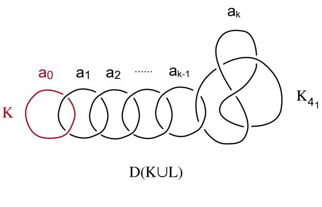
Let $(M,K)$ be a pair such that $M{\smallsetminus}K$ is homeomorphic to $S^{3}{\smallsetminus}K_{4_{1}}.$ Then $M$ is obtained from $S^{3}$ by doing a $\frac{p}{q}$ Dehn-filling along $K_{4_{1}}$ and $K$ is isotopic to a curve on the boundary of the tubular neighborhood of $K_{4_{1}}$ that intersects the $(p,q)$ -curve of the boundary at exactly one point. By eg. [25, p.273], $M$ can also be obtained by doing a surgery along a framed link $L$ of $k$ components with framings $a_{1},\dots,a_{k}$ coming from the continued fraction expansion

\frac{p}{q}=a_{k}-\frac{1}{a_{k-1}-\frac{1}{\cdots-\frac{1}{a_{1}}}}

of $\frac{p}{q},$ and $K$ is a framed trivial loop isotopic to the meridian of the last loop (see Figure 1).

Refer to caption — Figure 1: The Kirby diagram of $(M,K)$

Proposition 3.1.

For an odd integer $r\geqslant 3,$ the $r$ -th relative Reshetikin-Turaev invariant $\mathrm{RT}_{r}(M,K,m_{0})$ of the triple $(M,K,m_{0})$ at the root $q=e^{\frac{2\pi i}{r}}$ can be computed as

\begin{split}\mathrm{RT}_{r}(M,K,m_{0})=\kappa_{r}\sum_{m_{1},\dots,m_{k}=-\frac{r-2}{2}}^{\frac{r-2}{2}}\sum_{m=\max\{-m_{k},m_{k}\}}^{\frac{r-2}{2}}\Big{(}g^{+}_{r}(m_{1},\dots,m_{k},m)+g^{-}_{r}(m_{1},\dots,m_{k},m)\Big{)},\end{split}

where

\kappa_{r}=\frac{2^{k-3}}{{\sqrt{r^{k+1}}}}\Big{(}\sin\frac{2\pi}{r}\Big{)}^{k-1}e^{\big{(}3\sum_{i=0}^{k}a_{i}+\sigma(L)+2k-2\big{)}\frac{r\pi i}{4}+\big{(}-\sum_{i=0}^{k}a_{i}(1+\frac{1}{r})+\frac{3\sigma(L)}{r}+\frac{\sigma(L)}{4}\big{)}\pi i}

and

g^{\pm}_{r}(m_{1},\dots,m_{k},m)=\epsilon\Big{(}\frac{2\pi m_{k}}{r},\frac{2\pi m}{r}\Big{)}e^{-\frac{2\pi m_{k}i}{r}+\frac{r}{4\pi i}V^{\pm}_{r}\Big{(}\frac{2\pi m_{1}}{r},\dots,\frac{2\pi m_{k}}{r},\frac{2\pi m}{r}\Big{)}}

with $\epsilon$ and $V_{r}$ defined as follows. Let

x_{0}=\frac{2\pi}{r}\Big{(}\frac{r-2}{2}-m_{0}\Big{)}=\pi-\frac{2\pi}{r}-\frac{2\pi m_{0}}{r}.

(1)

If both $0<y\pm x_{k}<\pi,$ then $\epsilon(x_{k},y)=2$ and

V^{\pm}_{r}(x_{1},\dots,x_{k},y)=\pm 2x_{0}x_{1}-\sum_{i=0}^{k}a_{i}x_{i}^{2}-\sum_{i=1}^{k-1}2x_{i}x_{i+1}-2\pi x_{k}+4x_{k}y-\varphi_{r}\Big{(}\pi-y-x_{k}-\frac{\pi}{r}\Big{)}+\varphi_{r}\Big{(}y-x_{k}+\frac{\pi}{r}\Big{)}.

(2)

If $0<y+x_{k}<\pi$ and $\pi<y-x_{k}<2\pi,$ then $\epsilon(x_{k},y)=1$ and

V^{\pm}_{r}(x_{1},\dots,x_{k},y)=\pm 2x_{0}x_{1}-\sum_{i=0}^{k}a_{i}x_{i}^{2}-\sum_{i=1}^{k-1}2x_{i}x_{i+1}-2\pi x_{k}+4x_{k}y-\varphi_{r}\Big{(}\pi-y-x_{k}-\frac{\pi}{r}\Big{)}+\varphi_{r}\Big{(}y-x_{k}-\pi+\frac{\pi}{r}\Big{)}.

(3)

If $\pi<y+x_{k}<2\pi$ and $0<y-x_{k}<\pi,$ then $\epsilon(x_{k},y)=1$ and

V^{\pm}_{r}(x_{1},\dots,x_{k},y)=\pm 2x_{0}x_{1}-\sum_{i=0}^{k}a_{i}x_{i}^{2}-\sum_{i=1}^{k-1}2x_{i}x_{i+1}-2\pi x_{k}+4x_{k}y-\varphi_{r}\Big{(}2\pi-y-x_{k}-\frac{\pi}{r}\Big{)}+\varphi_{r}\Big{(}y-x_{k}+\frac{\pi}{r}\Big{)}.

Proof.

A direct computation shows that

\langle\mu_{r}\omega_{r}\rangle_{U_{+}}=e^{\big{(}-\frac{3}{r}-\frac{r+1}{4}\big{)}\pi i}.

Let

\kappa_{r}^{\prime}=\mu_{r}^{k+1}\langle\mu_{r}\omega_{r}\rangle_{U_{+}}^{-\sigma(L)}=\bigg{(}\frac{\sqrt{2}\sin\frac{2\pi}{r}}{\sqrt{r}}\bigg{)}^{k+1}e^{-\sigma(L)\big{(}-\frac{3}{r}-\frac{r+1}{4}\big{)}\pi i}.

Then by (2.1), we have

\begin{split}\mathrm{RT}_{r}(M)&=\kappa_{r}^{\prime}\langle e_{m_{0}},\omega_{r},\dots,\omega_{r}\rangle_{D(K\cup L)}\\ &=\kappa_{r}^{\prime}\sum_{m_{1},\dots,m_{k}=0}^{r-2}(-1)^{m_{0}+m_{k}+\sum_{i=0}^{k}a_{i}m_{i}}q^{\sum_{i=0}^{n}\frac{a_{i}m_{i}(m_{i}+2)}{2}}\prod_{i=0}^{k-1}[(m_{i}+1)(m_{i+1}+1)]\langle e_{m_{k}}\rangle_{D(K_{4_{1}})},\end{split}

where the second equality comes from the fact that $e_{n}$ is an eigenvector of the positive and the negative twist operator of eigenvalue $(-1)^{n}q^{\pm\frac{n(n+2)}{2}}$ , and is also an eigenvector of the circle operator $c(e_{m})$ (defined by enclosing $e_{n}$ by $e_{m}$ ) of eigenvalue $(-1)^{m}\frac{[(m+1)(n+1)]}{[n+1]}.$ By Habiro’s formula [11] (see also [19] for a skein theoretical computation)

\begin{split}\langle e_{n}\rangle_{D(K_{4_{1}})}=\frac{(-1)^{n+1}}{\{1\}}\sum_{m=0}^{\min\{n,r-2-n\}}q^{-2(n+1)(m+\frac{1}{2})}\frac{(q)_{n+1+m}}{(q)_{n-m}},\end{split}

where $\{n\}=q^{n}-q^{-n}$ and $(q)_{n}=\prod_{k=1}^{n}(1-q^{2k}).$

Then

\begin{split}\mathrm{RT}_{r}(M)=&\frac{(-1)^{m_{0}+1}}{\{1\}}\kappa_{r}^{\prime}\sum_{m_{1},\dots,m_{k}=0}^{r-2}\sum_{m=0}^{\min\{m_{k},r-2-m_{k}\}}(-1)^{\sum_{i=0}^{k}a_{i}m_{i}}q^{\sum_{i=1}^{n}\frac{a_{i}m_{i}(m_{i}+2)}{2}-2(m_{k}+1)(m+\frac{1}{2})}\\ &\quad\quad\quad\quad\quad\quad\quad\quad\quad\quad\quad\quad\prod_{i=0}^{k-1}[(m_{i}+1)(m_{i+1}+1)]\frac{(q)_{m_{k}+1+m}}{(q)_{m_{k}-m}}.\\ =&\frac{(-1)^{m_{0}+1}2^{k-1}}{\{1\}^{2}}\kappa_{r}^{\prime}\sum_{m_{1},\dots,m_{k}=0}^{r-2}\sum_{m=0}^{\min\{m_{k},r-2-m_{k}\}}\Big{(}q^{(m_{0}+1)(m_{1}+1)}-q^{-(m_{0}+1)(m_{1}+1)}\Big{)}\\ &\quad\quad(-1)^{\sum_{i=0}^{k}a_{i}m_{i}}q^{\sum_{i=0}^{k}\frac{a_{i}m_{i}(m_{i}+2)}{2}+\sum_{i=1}^{k-1}(m_{i}+1)(m_{i+1}+1)-2(m_{k}+1)(m+\frac{1}{2})}\frac{(q)_{m_{k}+1+m}}{(q)_{m_{k}-m}},\\ \end{split}

(3.1)

where the last equality comes from the following computation. For each $i\in\{1,\dots,k-1\}$ let $\epsilon_{i}\in\{0,1\},$ and let

\begin{split}&S^{(\epsilon_{1},\dots,\epsilon_{k-1})}(m_{1},\dots,m_{k-1})\\ =&\frac{(-1)^{m_{0}+1}}{\{1\}^{2}}\kappa_{r}^{\prime}\sum_{m_{k}=0}^{r-2}\sum_{m=0}^{\min\{m_{k},r-2-m_{k}\}}\Big{(}q^{(m_{0}+1)(m_{1}+1)}-q^{-(m_{0}+1)(m_{1}+1)}\Big{)}\\ &(-1)^{\sum_{i=0}^{k}a_{i}m_{i}+\sum_{i=1}^{k-1}\epsilon_{i}}q^{\sum_{i=0}^{k}\frac{a_{i}m_{i}(m_{i}+2)}{2}+\sum_{i=1}^{k-1}(-1)^{\epsilon_{i}}(m_{i}+1)(m_{i+1}+1)-2(m_{k}+1)(m+\frac{1}{2})}\frac{(q)_{m_{k}+1+m}}{(q)_{m_{k}-m}}.\end{split}

Then

\mathrm{RT}_{r}(M)=\sum_{m_{1},\dots,m_{k-1}=0}^{r-2}\sum_{\epsilon_{1},\dots,\epsilon_{k-1}\in\{0,1\}}S^{(\epsilon_{1},\dots,\epsilon_{k-1})}(m_{1},\dots,m_{k-1}).

For each $i\in\{1,\dots,,k-1\},$ a direct computation shows that

\begin{split}S^{(0,\dots,0,\epsilon_{i+1},\dots,\epsilon_{k-1})}&(m_{1},\dots,m_{i+1},\dots,m_{k-1})\\ &=S^{(0,\dots,0,1,\epsilon_{i+1},\dots,\epsilon_{k-1})}(r-2-m_{1},\dots,r-2-m_{i},m_{i+1},\dots,m_{k-1}).\end{split}

Then we have

\sum_{m_{1},\dots,m_{k-1}=0}^{r-2}S^{(0,\dots,0,\epsilon_{i+1},\dots,\epsilon_{k-1})}(m_{1},\dots,m_{k-1})=\sum_{m_{1},\dots,m_{k-1}=0}^{r-2}S^{(0,\dots,0,1,\epsilon_{i+1},\dots,\epsilon_{k-1})}(m_{1},\dots,m_{k-1}),

and hence

\mathrm{RT}_{r}(M)=2^{k-1}\sum_{m_{1},\dots,m_{k-1}=0}^{r-2}S^{(0,\dots,0)}(m_{1},\dots,m_{k-1}),

which proves (3.1).

Now let $m^{\prime}=\frac{r-2}{2}-m,$ and for each $i\in\{0,1,\dots,k\}$ let $m_{i}^{\prime}=\frac{r-2}{2}-m_{i}.$ Then

\begin{split}\mathrm{RT}_{r}(M)={\kappa_{r}}\sum_{m_{1}^{\prime},\dots,m_{k}^{\prime}=-\frac{r-2}{2}}^{\frac{r-2}{2}}&\sum_{m^{\prime}=\max\{-m_{k}^{\prime},m_{k}^{\prime}\}}^{\frac{r-2}{2}}\Big{(}q^{m_{0}^{\prime}m_{1}^{\prime}}+q^{-m_{0}^{\prime}m_{1}^{\prime}}\Big{)}\\ &(-1)^{m_{k}^{\prime}}q^{\sum_{i=0}^{k}\frac{a_{i}m_{i}^{\prime 2}}{2}+\sum_{i=1}^{k-1}{m_{i}^{\prime}m_{i+1}^{\prime}}-2m_{k}^{\prime}m^{\prime}-{m_{k}^{\prime}}}\frac{(q)_{r-1-m^{\prime}-m_{k}^{\prime}}}{(q)_{m^{\prime}-m_{k}^{\prime}}},\\ \end{split}

and by Lemma 2.4,

\mathrm{RT}_{r}(M)=\kappa_{r}\sum_{m_{1}^{\prime},\dots,m_{k}^{\prime}=-\frac{r-2}{2}}^{\frac{r-2}{2}}\sum_{m^{\prime}=\max\{-m_{k}^{\prime},m_{k}^{\prime}\}}^{\frac{r-2}{2}}\Big{(}g^{+}_{r}(m_{1}^{\prime},\dots,m_{k}^{\prime},m^{\prime})+g^{-}_{r}(m_{1}^{\prime},\dots,m_{k}^{\prime},m^{\prime})\Big{)}.

∎

4 Poisson summation formula

We notice that the summation in Proposition 3.1 is finite, and to use the Poisson summation formula, we need an infinite sum over integral points. To this end, we consider the following regions and a bump function over them.

Let $x_{i}=\frac{2\pi m_{i}}{r}$ for each $i\in\{1,\dots,k\},$ and let $y=\frac{2\pi m}{r}.$ For $\delta\geqslant 0,$ we let

D_{\delta}=\Big{\{}(x,y)\in\mathbb{R}^{2}\ \Big{|}\ \delta<y+x<\frac{\pi}{2}-\delta,\delta<y-x<\frac{\pi}{2}-\delta\Big{\}},

D^{\prime}_{\delta}=\Big{\{}(x,y)\in\mathbb{R}^{2}\ \Big{|}\ \delta<y+x<\frac{\pi}{2}-\delta,\pi+\delta<y-x<\frac{3\pi}{2}-\delta\Big{\}}

and

D^{\prime\prime}_{\delta}=\Big{\{}(x,y)\in\mathbb{R}^{2}\ \Big{|}\ \pi+\delta<y+x<\frac{3\pi}{2}-\delta,\delta<y-x<\frac{\pi}{2}-\delta\Big{\}},

and let $\mathcal{D}_{\delta}=D_{\delta}\cup D^{\prime}_{\delta}\cup D^{\prime\prime}_{\delta}.$ If $\delta=0,$ we omit the subscript and write $D=D_{0},$ $D^{\prime}=D^{\prime}_{0},$ $D^{\prime\prime}=D^{\prime\prime}_{0}$ and $\mathcal{D}=D\cup D^{\prime}\cup D^{\prime\prime}.$

For a sufficiently small $\delta>0,$ we consider a $C^{\infty}$ -smooth bump function $\psi$ on $\mathbb{R}^{k+1}$ such that

\left\{\begin{array}[]{rl}\psi(x_{1},\dots,x_{k},y)=1,&(x_{1},\dots,x_{k},y)\in[-\pi+\frac{2\pi}{r},\pi-\frac{2\pi}{r}]^{k-1}\times\overline{\mathcal{D}_{\frac{\delta}{2}}}\\ 0<\psi(x_{1},\dots,x_{k},y)<1,&(x_{1},\dots,x_{k},y)\in(-\pi,\pi)^{k-1}\times\mathcal{D}{\smallsetminus}[-\pi+\frac{2\pi}{r},\pi-\frac{2\pi}{r}]^{k-1}\times\overline{\mathcal{D}_{\frac{\delta}{2}}}\\ \psi(x_{1},\dots,x_{k},y)=0,&(x_{1},\dots,x_{k},y)\notin(-\pi,\pi)^{k-1}\times\mathcal{D},\\ \end{array}\right.

and let

f^{\pm}_{r}(m_{1},\dots,m_{k},m)=\psi\Big{(}\frac{2\pi m_{1}}{r},\dots,\frac{2\pi m_{k}}{r},\frac{2\pi m}{r}\Big{)}g^{\pm}_{r}(m_{1},\dots,m_{k},m).

Then by Proposition 4.2, we have

\mathrm{RT}_{r}(M)=\kappa_{r}\sum_{(m_{1},\dots,m_{k},m)\in(\mathbb{Z}+\frac{1}{2})^{k+1}}\Big{(}f^{+}_{r}(m_{1},\dots,m_{k},m)+f^{-}_{r}(m_{1},\dots,m_{k},m)\Big{)}+\text{error term}.

(4.1)

Since $f^{\pm}_{r}$ is $C^{\infty}$ -smooth and equals zero out of $D,$ it is in the Schwartz space on $\mathbb{R}^{k+1}.$ Recall that by the Poisson Summation Formula (see e.g. [26, Theorem 3.1]), for any function $f$ in the Schwartz space on $\mathbb{R}^{k},$

\sum_{(m_{1},\dots,m_{k})\in\mathbb{Z}^{k}}f(m_{1},\dots,m_{k})=\sum_{(n_{1},\dots,n_{k})\in\mathbb{Z}^{k}}\hat{f}(n_{1},\dots,n_{k}),

where $\hat{f}(n_{1},\dots,n_{k})$ is the $(n_{1},\dots,n_{k})$ -th Fourier coefficient of $f$ defined by

\widehat{f^{\pm}}(n_{1},\dots,n_{k})=\int_{\mathbb{R}^{k}}f^{\pm}(m_{1},\dots,m_{k})e^{\sum_{j=1}^{k}2\pi in_{j}m_{j}}dm_{1}\dots dm_{k}.

As a consequence, we have

Proposition 4.1.

\mathrm{RT}_{r}(M)=\kappa_{r}\sum_{(n_{1},\dots,n_{k},n)\in\mathbb{Z}^{k+1}}\Big{(}\widehat{f^{+}}(n_{1},\dots,n_{k})+\widehat{f^{-}}(n_{1},\dots,n_{k})\Big{)}+\text{error term},

where

\begin{split}\widehat{f^{\pm}_{r}}(n_{1},\dots,n_{k},n)=(-1)^{\sum_{i=1}^{k}n_{i}+n}\Big{(}\frac{r}{2\pi}\Big{)}^{k+1}&\int_{(-\pi,\pi)^{k-1}\times\mathcal{D}}\psi(x_{1},\dots,x_{k},y)\epsilon(x_{k},y)\\ &e^{-x_{k}i+\frac{r}{4\pi i}\Big{(}V^{\pm}_{r}(x_{1},\dots,x_{k},y)-4\pi\sum_{i=1}^{k}n_{i}x_{k}-4\pi ny\Big{)}}dx_{1}\dots dx_{k}dy.\end{split}

Proof.

To apply the Poisson Summation Formula, we need to make the sum in (4.1) over integers instead of half-integers. To do this, we let $m_{i}^{\prime}=m_{i}+\frac{1}{2}$ for $i=1,\dots,k$ and let $m^{\prime}=m+\frac{1}{2}.$ Then

\sum_{(m_{1},\dots,m_{k},m)\in(\mathbb{Z}+\frac{1}{2})^{k+1}}f^{\pm}_{r}(m_{1},\dots,m_{k},m)=\sum_{(m^{\prime}_{1},\dots,m^{\prime}_{k},m^{\prime})\in\mathbb{Z}^{k+1}}f^{\pm}_{r}\Big{(}m^{\prime}_{1}-\frac{1}{2},\dots,m^{\prime}_{k}-\frac{1}{2},m^{\prime}-\frac{1}{2}\Big{)}.

Now by the Poisson Summation Formula, the right hand side equals

\sum_{(n_{1},\dots,n_{k},n)\in\mathbb{Z}^{k+1}}\int_{\mathbb{R}^{k+1}}f^{\pm}_{r}\Big{(}m^{\prime}_{1}-\frac{1}{2},\dots,m^{\prime}_{k}-\frac{1}{2},m^{\prime}-\frac{1}{2}\Big{)}e^{\sum_{j=1}^{k}2\pi in_{j}m^{\prime}_{j}+2\pi inm^{\prime}}dm^{\prime}_{1}\dots dm^{\prime}_{k}dm^{\prime}.

Finally, using the change of variable $x_{i}=\frac{2\pi m_{i}}{r}=\frac{2\pi m^{\prime}_{i}}{r}-\frac{\pi}{r}$ for $i=1,\dots,k$ and $y=\frac{2\pi m}{r}=\frac{2\pi m^{\prime}}{r}-\frac{\pi}{r},$ we get the result. ∎

We will give a preliminary estimate of the Fourier coefficients in Section 5 simplifying them to a $2$ -dimensional integral which will be further estimated in Sections 7.3 and 7.2, and estimate the error term in Proposition 4.1 as follows.

Proposition 4.2.

For $\epsilon>0,$ we can choose a sufficiently small $\delta>0$ so that if one of $m+m_{k}$ and $m-m_{k}$ is not in $\big{(}\frac{\delta r}{2\pi},\frac{r}{4}-\frac{\delta r}{2\pi}\big{)}\cup\big{(}\frac{r}{2}+\frac{\delta r}{2\pi},\frac{3r}{4}-\frac{\delta r}{2\pi}\big{)},$ then

|g_{r}(m_{1},\dots,m_{k},m)|<O\Big{(}e^{\frac{r}{4\pi}\big{(}\frac{1}{2}\mathrm{Vol}(\mathrm{S}^{3}{\smallsetminus}K_{4_{1}})+\epsilon\big{)}}\Big{)}.

As a consequence, the error term in Proposition 4.1 is of order at most $O\Big{(}e^{\frac{r}{4\pi}\big{(}\frac{1}{2}\mathrm{Vol}(\mathrm{S}^{3}{\smallsetminus}K_{4_{1}})+\epsilon\big{)}}\Big{)}.$

To prove Proposition 4.2, we need the following estimate, which first appeared in [10, Proposition 8.2] for $t=e^{\frac{2\pi i}{r}},$ and for the root $t=e^{\frac{4\pi i}{r}}$ in [6, Proposition 4.1].

Lemma 4.3.

For any integer $0<n<r$ and at $t=e^{\frac{4\pi i}{r}},$

\log\left|\{n\}!\right|=-\frac{r}{2\pi}\Lambda\left(\frac{2n\pi}{r}\right)+O\left(\log(r)\right).

Proof of Proposition 4.2.

We have

|g^{\pm}_{r}(m_{1},\dots,m_{k},m)|=\Big{|}\sin\Big{(}\frac{2\pi m_{1}}{r}\Big{)}\epsilon\Big{(}\frac{2\pi m_{k}}{r},\frac{2\pi m}{r}\Big{)}\Big{|}\Big{|}\frac{\{r-1-m-m_{k}\}!}{\{m-m_{k}\}!}\Big{|},

and by Lemma 4.3, we have

\log|g^{\pm}_{r}(m_{1},\dots,m_{k},m)|=-\frac{r}{2\pi}\Lambda\Big{(}\frac{2\pi(r-1-m-m_{k})}{r}\Big{)}+\frac{r}{2\pi}\Lambda\Big{(}\frac{2\pi(m-m_{k})}{r}\Big{)}+O(\log(r)).

Choose $\delta>0$ so that

\Lambda(\delta)<\frac{\epsilon}{4}.

Now if one of $m+m_{k}$ and $m-m_{k}$ is not in $\big{(}\frac{\delta r}{2\pi},\frac{r}{4}-\frac{\delta r}{2\pi}\big{)}\cup\big{(}\frac{r}{2}+\frac{\delta r}{2\pi},\frac{3r}{4}-\frac{\delta r}{2\pi}\big{)},$ then

\log|g^{\pm}_{r}(m_{1},\dots,m_{k},m)|<\frac{r}{2\pi}\Big{(}\Lambda\Big{(}\frac{\pi}{6}\Big{)}+\frac{\epsilon}{2}\Big{)}=\frac{r}{4\pi}\Big{(}\frac{1}{2}\mathrm{Vol}(\mathrm{S}^{3}{\smallsetminus}K_{4_{1}})+\epsilon\Big{)}.

The last equality is true because by properties of the Lobachevsky function $\Lambda\big{(}\frac{\pi}{6}\big{)}=\frac{3}{2}\Lambda\big{(}\frac{\pi}{3}\big{)},$ and the volume of $\mathrm{S}^{3}{\smallsetminus}K_{4_{1}}$ equals $6\Lambda(\frac{\pi}{3}).$ ∎

5 A simplification of the Fourier coefficients

The main results of this Section are Propositions 5.4 and 5.7 below, which simplify the Fourier coefficients $\hat{f}_{r}(n_{1},\dots,n_{k},n).$

We consider the continued fraction expansion

\frac{p}{q}=a_{k}-\frac{1}{a_{k-1}-\frac{1}{\cdots-\frac{1}{a_{1}}}}

of $\frac{p}{q}$ with the requirement that $a_{i}\geqslant 2$ for $i=1,\dots a_{k-1}.$ For each $i\leqslant k-1,$ we let

b_{i}=a_{i}-\frac{1}{a_{i-1}-\frac{1}{\cdots-\frac{1}{a_{1}}}},

and let

c_{i}=\prod_{j=1}^{i}b_{i}.

Then $c_{1}=b_{1}=a_{1}\geqslant 2,$ $b_{k}=\frac{p}{q},$ $c_{k-1}=q,$ and $b_{i}>1$ and $c_{i}>c_{i-1}\geqslant 2$ for any $i\leqslant k-1.$ We need the following Lemmas.

Lemma 5.1.

[28, Lemma 5.1] Let $(p^{\prime},q^{\prime})$ be the a unique pair such that $pp^{\prime}+qq^{\prime}=1$ and $-q<p^{\prime}\leqslant 0.$ Then

\sum_{j=1}^{k-1}\frac{1}{c_{j-1}c_{j}}=-\frac{p^{\prime}}{q}.

Lemma 5.2.

[28, Lemma 5.2] Let $\beta\in\mathbb{R}{\smallsetminus}\{0\}.$

(1)

If $\alpha\in(a,b),$ then

\int_{a}^{b}e^{\frac{r}{4\pi i}\beta(x-\alpha)^{2}}dx=\frac{2\pi\sqrt{i}}{\sqrt{\beta}}\frac{1}{\sqrt{r}}\Big{(}1+O\Big{(}\frac{1}{\sqrt{r}}\Big{)}\Big{)}.

(2)

If $\alpha\in\mathbb{R}{\smallsetminus}(a,b),$ then

$\Big{|}\int_{a}^{b}e^{\frac{r}{4\pi i}\beta(x-\alpha)^{2}}dx\Big{|}\leqslant O\Big{(}\frac{1}{r}\Big{)}.$

By completing the squares, we have on $D$

\begin{split}V^{+}_{r}(x_{1},\dots,x_{k},y)=&-\sum_{i=1}^{k-1}b_{i}\Big{(}x_{i}+\frac{x_{i+1}}{b_{i}}+(-1)^{i}\frac{x_{0}}{c_{i}}\Big{)}^{2}+\sum_{i=1}^{k-1}\frac{x_{0}^{2}}{c_{i-1}c_{i}}-a_{0}x_{0}^{2}\\ &-\frac{px_{k}^{2}}{q}-\frac{(-1)^{k}2x_{0}x_{k}}{q}-2\pi x_{k}+4x_{k}y-\varphi_{r}\Big{(}\pi-x_{k}-y-\frac{\pi}{r}\Big{)}+\varphi_{r}\Big{(}y-x_{k}+\frac{\pi}{r}\Big{)},\\ \end{split}

and

\begin{split}V^{-}_{r}(x_{1},\dots,x_{k},y)=&-\sum_{i=1}^{k-1}b_{i}\Big{(}x_{i}+\frac{x_{i+1}}{b_{i}}-(-1)^{i}\frac{x_{0}}{c_{i}}\Big{)}^{2}+\sum_{i=1}^{k-1}\frac{x_{0}^{2}}{c_{i-1}c_{i}}-a_{0}x_{0}^{2}\\ &-\frac{px_{k}^{2}}{q}+\frac{(-1)^{k}2x_{0}x_{k}}{q}-2\pi x_{k}+4x_{k}y-\varphi_{r}\Big{(}\pi-x_{k}-y-\frac{\pi}{r}\Big{)}+\varphi_{r}\Big{(}y-x_{k}+\frac{\pi}{r}\Big{)},\\ \end{split}

and with the corresponding change of the variables in $\varphi_{r}$ on $D^{\prime}$ and $D^{\prime\prime}.$

From now on, we will let $x=x_{k}.$ Then solving the system of the critical equations

x_{i}+\frac{x_{i+1}}{b_{i}}\pm(-1)^{i}\frac{x_{0}}{c_{i}}=0

for $x_{i}$ ’s in terms of $x,$ we have for every $i$ in $\{1,\dots,k\}$

x^{\pm}_{i}(x)=(-1)^{k-i}c_{i-1}\Big{(}\frac{x}{q}\pm(-1)^{k}\sum_{j=i}^{k-1}\frac{x_{0}}{c_{j-1}c_{j}}\Big{)},

and in particular, by Lemma 5.1,

x^{\pm}_{1}(x)=\frac{(-1)^{k-1}x\pm p^{\prime}x_{0}}{q}.

Now we start to simplify the Fourier coefficients. We need the following

Lemma 5.3.

If $-\pi+\frac{q\pi}{r}<x<\pi-\frac{q\pi}{r},$ then $-\pi+\frac{2\pi}{r}<x^{\pm}_{i}(x)<\pi-\frac{2\pi}{r}$ for each $i\in\{1,\dots,k-1\}.$

Proof.

We use a backward induction to prove a stronger statement that

-\pi+\frac{c_{i-1}\pi}{r}<x^{\pm}_{i}(x)<\pi-\frac{c_{i-1}\pi}{r}

for each $i.$ We first note that $|x_{0}|\leqslant\pi.$

For $x^{\pm}_{k-1}(x),$ we have

\begin{split}|x^{\pm}_{k-1}(x)|&=\Big{|}\frac{x}{b_{k-1}}\pm\frac{x_{0}}{c_{k-1}}\Big{|}=\Big{|}\frac{c_{k-2}x}{c_{k-1}}\pm\frac{x_{0}}{c_{k-1}}\Big{|}\\ &\leqslant\frac{c_{k-2}\pi+|x_{0}|-\frac{c_{k-2}q\pi}{r}}{c_{k-1}}\leqslant\frac{(c_{k-2}+1)\pi-\frac{c_{k-2}q\pi}{r}}{c_{k-1}}\leqslant\pi-\frac{c_{k-2}\pi}{r},\end{split}

where the last inequality comes from that $q=c_{k-1}>c_{k-2},$ hence $q\geqslant c_{k-2}+1.$

Now assume the result holds for $x^{\pm}_{i+1}(x)$ that $-\pi+\frac{c_{i}\pi}{r}<x^{\pm}_{i+1}(x)<\pi-\frac{c_{i}\pi}{r},$ then

\begin{split}|x^{\pm}_{i}(x)|&=\Big{|}\frac{x^{\pm}_{i+1}}{b_{i}}\pm\frac{x_{0}}{c_{i}}\Big{|}=\Big{|}\frac{c_{i-1}x^{\pm}_{i+1}}{c_{i}}\pm\frac{x_{0}}{c_{i}}\Big{|}\\ &\leqslant\frac{c_{i-1}\pi+|x_{0}|-\frac{c_{i-1}c_{i}\pi}{r}}{c_{i}}\leqslant\frac{(c_{i-1}+1)\pi-\frac{c_{i-1}c_{i}\pi}{r}}{c_{i}}\leqslant\pi-\frac{c_{i-1}\pi}{r},\end{split}

where the last inequality comes from that $c_{i}>c_{i-1},$ hence $c_{i}\geqslant c_{i-1}+1.$ ∎

Proposition 5.4.

\hat{f}^{\pm}_{r}(0,0,\dots,0)=\frac{i^{-\frac{k-1}{2}}r^{\frac{k+3}{2}}}{4\pi^{2}\sqrt{q}}\Big{(}\int_{\mathcal{D}_{\frac{\delta}{2}}}\epsilon(x,y)e^{-xi+\frac{r}{4\pi i}V^{\pm}_{r}(x,y)}dxdy\Big{)}\Big{(}1+O\Big{(}\frac{1}{\sqrt{r}}\Big{)}\Big{)},

where

V_{r}^{\pm}(x,y)=\frac{-px^{2}\pm(-1)^{k}2x_{0}x}{q}-2\pi x+4xy-\varphi_{r}\Big{(}\pi-y-x_{k}-\frac{\pi}{r}\Big{)}+\varphi_{r}\Big{(}y-x_{k}+\frac{\pi}{r}\Big{)}-\Big{(}\frac{p^{\prime}}{q}+a_{0}\Big{)}x_{0}^{2},

on $D,$ and with the corresponding change of the variables in $\varphi_{r}$ on $D^{\prime}$ and $D^{\prime\prime}.$

Proof.

For $(x,y)\in\mathcal{D}_{\frac{\delta}{2}},$ since $-\pi+\frac{q\pi}{r}<x<\pi-\frac{q\pi}{r},$ iteratively using Lemma 5.2 (1) and Lemma 5.3 to the variables $x_{1},\dots,x_{k-1},$ we get the estimate. On the region $\big{(}(-\pi,\pi)^{k-1}{\smallsetminus}[-\pi+\frac{2\pi}{r},\pi-\frac{2\pi}{r}]^{k-1}\big{)}\times\mathcal{D}_{\frac{\delta}{2}}$ where the bump function makes a difference, by Lemma 5.3, for at least one variable $x_{i}$ Lemma 5.2 (2) applies. Hence the contribution there is of order at most $O\big{(}\frac{1}{\sqrt{r}})$ times the whole integral. ∎

In Section 7, we will show that $\widehat{f^{\pm}}(0,0,\dots,0)$ are the only leading Fourier coefficients, ie., have the largest growth rate.

The other Fourier coefficients can be simplified similarly. By a completion of the squares, we have

\begin{split}&V^{\pm}_{r}(x_{1},\dots,x_{k-1},x,y)-4\pi\sum_{i=1}^{k-1}n_{i}x_{i}-4\pi k_{1}x-4\pi k_{2}y\\ =&-\sum_{i=1}^{k-1}b_{i}\Big{(}x_{i}+\frac{x_{i+1}}{b_{i}}+\sum_{j=1}^{i}(-1)^{i-j}\frac{2n_{j}c_{j-1}\pi}{c_{i}}\pm(-1)^{i}\frac{x_{0}}{c_{i}}\Big{)}^{2}+C\\ &-\frac{px^{2}}{q}\mp\frac{(-1)^{k}2x_{0}x}{q}-2\pi x+4xy-\varphi_{r}\Big{(}\pi-x-y-\frac{\pi}{r}\Big{)}+\varphi_{r}\Big{(}y-x+\frac{\pi}{r}\Big{)}\\ &-\frac{4\pi k_{0}x}{q}-4\pi k_{1}x-4\pi k_{2}y,\\ \end{split}

on $D,$ where $C$ is a real constant depending on $(n_{1},\dots,n_{k-1}),$ and

k_{0}=\sum_{j=1}^{k-1}(-1)^{k-j}n_{j}c_{j-1}.

On $D^{\prime}$ and $D^{\prime\prime}$ there is a corresponding change of the variables in $\varphi_{r}.$

Solving the system of the critical equations

x_{i}+\frac{x_{i+1}}{b_{i}}+\sum_{j=1}^{i}(-1)^{i-j}\frac{2n_{j}c_{j-1}\pi}{c_{i}}\pm(-1)^{i}\frac{x_{0}}{c_{i}}=0,

we can write each $x_{i}$ as a function $x^{\pm}_{i}(x)$ of $x.$

Iteratively using Lemma 5.2, we have

Proposition 5.5.

Let

V_{r}^{\pm,(k_{0},k_{1},k_{2})}(x,y)=V_{r}^{\pm}(x,y)-\frac{4k_{0}\pi x}{q}-4k_{1}\pi x-4k_{2}\pi y+C,

where $C$ is a real constant depending on $(n_{1},\dots,n_{k-1}).$ Then

\begin{split}|\widehat{f^{\pm}_{r}}(n_{1},\dots,n_{k-1},k_{1},k_{2})|\leqslant O\Big{(}r^{\frac{k+3}{2}}\Big{)}\Big{|}\int_{\mathcal{D}_{\frac{\delta}{2}}}e^{\frac{r}{4\pi i}V_{r}^{\pm,(k_{0},k_{1},k_{2})}(x,y)}dxdy\Big{|}.\end{split}

Moreover, if for each $x\in(-\pi,\pi),$ there is some $i\in\{1,\dots,k-1\}$ such that $x^{\pm}_{i}(x)\notin(-\pi,\pi),$ then

\begin{split}|\widehat{f^{\pm}_{r}}(n_{1},,\dots,n_{k-1},k_{1},k_{2})|\leqslant O\Big{(}r^{\frac{k+2}{2}}\Big{)}\Big{|}\int_{\mathcal{D}_{\frac{\delta}{2}}}e^{\frac{r}{4\pi i}V_{r}^{\pm,(k_{0},k_{1},k_{2})}(x,y)}dxdy\Big{|}.\end{split}

The following lemma will be need later in estimating the growth rate of the invariants.

Lemma 5.6.

(1)

If $(n_{1},\dots,n_{k-1})\neq(0,\dots,0)$ and $k_{0}=0,$ then for each $x\in(-\pi,\pi)$ there is some $i\in\{1,\dots,k-1\}$ so that $x^{+}_{i}(x)\notin(-\pi,\pi),$ and some $j\in\{1,\dots,k-1\}$ so that $x^{-}_{j}(x)\notin(-\pi,\pi).$
(2)

If $(n_{1},\dots,n_{k-1})\neq(0,\dots,0)$ and $|k_{0}|\geqslant q,$ then $x^{\pm}_{k-1}(x)\notin(-\pi,\pi)$ for all $x\in(-\pi,\pi).$

Proof.

We prove (1) and (2) for $x^{+}_{i}(x),$ and that for $x^{-}_{j}(x)$ is similar.

For (1), let $x\in(-\pi,\pi)$ and let $n_{i_{0}}$ be the last non-zero number in $n_{i}$ ’s, ie. $n_{i_{0}}\neq 0$ and $n_{j}=0$ for all $j>i_{0}.$ Then $i_{0}\geqslant 2$ since otherwise $n_{i_{0}}=n_{1}=(-1)^{k-1}k_{0}=0,$ which is a contradiction.

If $x^{+}_{i_{0}}(x)\notin(-\pi,\pi),$ then we are done.

If $x^{+}_{i_{0}}(x)\in(-\pi,\pi),$ then we have

\Big{|}\frac{x^{+}_{i_{0}}(x)}{b_{i_{0}-1}}\pm\frac{x_{0}}{c_{i_{0}-1}}\Big{|}<\frac{\pi}{b_{i_{0}-1}}+\frac{\pi}{c_{i_{0}-1}}=\frac{c_{i_{0}-2}+1}{c_{i_{0}-1}}\pi\leqslant\pi,

where the equality and the last inequality come from that $c_{i}=b_{i}c_{i-1}$ and $c_{i-1}+1\leqslant c_{i}.$

Since

|k_{0}|=\Big{|}\sum_{j=1}^{i_{0}}(-1)^{j}n_{j}c_{j-1}\Big{|}=|n_{i_{0}}c_{i_{0}-1}|-\Big{|}\sum_{j=1}^{i_{0}-1}(-1)^{j}n_{j}c_{j-1}\Big{|}=0,

we have

\Big{|}\sum_{j=1}^{i_{0}-1}(-1)^{j}\frac{n_{j}c_{j-1}}{c_{i_{0}-1}}\Big{|}=|n_{i_{0}}|.

Then

\begin{split}|x^{+}_{i_{0}-1}|&=\Big{|}\frac{x^{+}_{i_{0}}(x)}{b_{i_{0}-1}}+\sum_{j=1}^{i_{0}-1}(-1)^{i_{0}-1-j}\frac{2n_{j}c_{j-1}\pi}{c_{i_{0}-1}}-(-1)^{i_{0}-1}\frac{x_{0}}{c_{i_{0}-1}}\Big{|}\\ &\geqslant\bigg{|}\Big{|}\sum_{j=1}^{i_{0}-1}(-1)^{j}\frac{2n_{j}c_{j-1}\pi}{c_{i_{0}-1}}\Big{|}-\Big{|}\frac{x^{+}_{i_{0}}(x)}{b_{i_{0}-1}}-(-1)^{i_{0}-1}\frac{x_{0}}{c_{i_{0}-1}}\Big{|}\bigg{|}\\ &\geqslant 2|n_{i_{0}}|\pi-\pi\geqslant\pi.\end{split}

The proof for (2) is similar. Since $-\pi<x<\pi,$ we have

\Big{|}\frac{x}{b_{k-1}}\pm\frac{x_{0}}{q}\Big{|}<\frac{\pi}{b_{k-1}}+\frac{\pi}{q}=\frac{c_{k-2}+1}{q}\pi\leqslant\pi.

If $|k_{0}|\geqslant q,$ then

\begin{split}|x^{\pm}_{k-1}|&=\Big{|}\frac{x}{b_{k-1}}+\frac{2k_{0}\pi}{q}\pm(-1)^{k-1}\frac{x_{0}}{q}\Big{|}\\ &\geqslant\bigg{|}\Big{|}\frac{2k_{0}\pi}{q}\Big{|}-\Big{|}\frac{x}{b_{k-1}}\pm(-1)^{k-1}\frac{x_{0}}{q}\Big{|}\bigg{|}\geqslant 2\pi-\pi=\pi.\end{split}

∎

Let

\widehat{F^{\pm}_{r}}(k_{0},k_{1},k_{2})=\int_{\mathcal{D}_{\frac{\delta}{2}}}e^{\frac{r}{4\pi i}V_{r}^{\pm,(k_{0},k_{1},k_{2})}(x,y)}dxdy.

Then by Propositions 5.5 and Lemma 5.6, we have the following

Proposition 5.7.

(1)

For $(n_{1},\dots,n_{k},n)\neq(0,\dots,0),$

\begin{split}\Big{|}\widehat{f^{\pm}_{r}}(n_{1},\dots,n_{k},n)\Big{|}\leqslant O\Big{(}r^{\frac{k+3}{2}}\Big{)}\Big{|}\widehat{F^{\pm}_{r}}(k_{0},k_{1},k_{2})\Big{|}.\end{split}

(2)

If $(n_{1},\dots,n_{k},n)\neq(0,\dots,0)$ with $k_{0}=0$ or with $|k_{0}|\geqslant q,$ then

\begin{split}\Big{|}\widehat{f^{\pm}_{r}}(n_{1},\dots,n_{k},n)\Big{|}\leqslant O\Big{(}r^{\frac{k+2}{2}}\Big{)}\Big{|}\widehat{F^{\pm}_{r}}(k_{0},k_{1},k_{2})\Big{|}.\end{split}

The integrals $\hat{F}_{r}(k_{0},k_{1},k_{2})$ will be further estimated in Section 7.

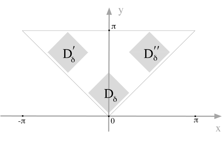
We notice that $V_{r}^{\pm}(x,y)$ and $V_{r}^{\pm,(k_{0},k_{1},k_{2})}(x,y)$ define holomorphic functions on the following regions $D_{\mathbb{C},\delta},$ $D^{\prime}_{\mathbb{C},\delta}$ and $D^{\prime\prime}_{\mathbb{C},\delta}$ of $\mathbb{C}^{2},$ where for $\delta\geqslant 0,$

D_{\mathbb{C},\delta}=\Big{\{}(x,y)\in\mathbb{C}^{2}\ \Big{|}\ \delta<\mathrm{Re}(y)+\mathrm{Re}(x)<\frac{\pi}{2}-\delta,\delta<\mathrm{Re}(y)-\mathrm{Re}(x)<\frac{\pi}{2}-\delta\Big{\}},

D^{\prime}_{\mathbb{C},\delta}=\Big{\{}(x,y)\in\mathbb{C}^{2}\ \Big{|}\ \delta<\mathrm{Re}(y)+\mathrm{Re}(x)<\frac{\pi}{2}-\delta,\pi+\delta<\mathrm{Re}(y)-\mathrm{Re}(x)<\frac{3\pi}{2}-\delta\Big{\}}

and

D^{\prime\prime}_{\mathbb{C},\delta}=\Big{\{}(x,y)\in\mathbb{C}^{2}\ \Big{|}\ \pi+\delta<\mathrm{Re}(y)+\mathrm{Re}(x)<\frac{3\pi}{2}-\delta,\delta<\mathrm{Re}(y)-\mathrm{Re}(x)<\frac{\pi}{2}-\delta\Big{\}}.

When $\delta=0,$ we denote the corresponding regions by $D_{\mathbb{C}},$ $D^{\prime}_{\mathbb{C}}$ and $D^{\prime\prime}_{\mathbb{C}}.$

We consider the following holomorphic functions

V^{\pm}(x,y)=\frac{-px^{2}\pm 2x_{0}x}{q}-2\pi x+4xy-\mathrm{Li}_{2}(e^{-2i(y+x)})+\mathrm{Li}_{2}(e^{2i(y-x)})-\Big{(}\frac{p^{\prime}}{q}+a_{0}\Big{)}x_{0}^{2}

on $D_{\mathbb{C}},$ $D^{\prime}_{\mathbb{C}}$ and $D^{\prime\prime}_{\mathbb{C}},$ which will play a crucial role in Section 7 in the estimate of the Fourier coefficients.

6 Geometry of the critical points

The main result of this Section is Proposition 6.3 which shows that the critical value of the functions $V^{\pm}$ defined in the previous section has real part the volume of $M_{K_{\theta}}$ and imaginary part the Chern-Simons invariant of $M_{K_{\theta}}$ as defined in Section 2.2. The key observation is Lemma 6.1 that the system of critical point equations of $V^{\pm}$ is equivalent to the system of hyperbolic gluing equations (consisting of an edge equation and an equation of the $\frac{p}{q}$ Dehn-filling with prescribed cone angle) for a particular ideal triangulation of the figure- $8$ knot complement.

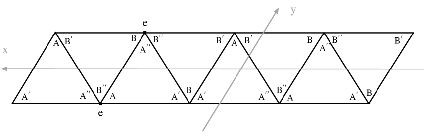
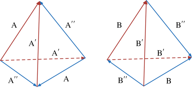
According to Thurston’s notes [27], the complement of the figure- $8$ knot has an ideal triangulation as drawn in Figure 3. We let $A$ and $B$ be the shape parameters of the two ideal tetrahedra and let $A^{\prime}=\frac{1}{1-A},$ $A^{\prime\prime}=1-\frac{1}{A},$ $B^{\prime}=\frac{1}{1-B}$ and $B^{\prime\prime}=1-\frac{1}{B}.$

In Figure 4 is a fundamental domain of the boundary of a tubular neighborhood of $K_{4_{1}}.$

Recall that for $z\in\mathbb{C}{\smallsetminus}(-\infty,0],$ the logarithmic function is defined by

\log z=\ln|z|+i\arg z

with $-\pi<\arg z<\pi.$

Then the holonomy around the edge $e$ is

\mathrm{H}(e)=\log A+2\log A^{\prime\prime}+\log B+2\log B^{\prime\prime},

and the holonomies of the curves $x$ and $y$ are respectively

\mathrm{H}(x)=2\log B+2\log B^{\prime\prime}-2\log A-2\log A^{\prime\prime}

and

\mathrm{H}(y)=\log B^{\prime}-\log A^{\prime\prime}.

By [27], we can choose the meridian $m=y$ and the longitude $l=x+2y.$ Hence

\mathrm{H}(m)=\log B^{\prime}-\log A^{\prime\prime},

and

\begin{split}\mathrm{H}(l)=2\pi i-2\log A-4\log A^{\prime\prime}.\end{split}

Then for the incomplete hyperbolic metric that gives the hyperbolic cone metric with cone angle $\theta,$ the system of hyperbolic gluing equations

\left\{\begin{array}[]{l}\mathrm{H}(e)=2\pi i\\ \\ p\mathrm{H}(m)+q\mathrm{H}(l)=\theta i\end{array}\right.

can be written as

\left\{\begin{array}[]{l}\log A+2\log A^{\prime\prime}+\log B+2\log B^{\prime\prime}=2\pi i\\ \\ p(\log B^{\prime}-\log A^{\prime\prime})+q(2\pi i-2\log A-4\log A^{\prime\prime})=\theta i.\end{array}\right.

(6.1)

From now on, we let $\theta=|2x_{0}|$ and, by switching the $+$ and $-$ if necessary, let

V^{\pm}(x,y)=\frac{-px^{2}\pm\theta x}{q}-2\pi x+4xy-\mathrm{Li}_{2}(e^{-2i(y+x)})+\mathrm{Li}_{2}(e^{2i(y-x)})-\Big{(}\frac{p^{\prime}}{q}+a_{0}\Big{)}\frac{\theta^{2}}{4}.

Taking partial derivatives of $V^{\pm},$ we have

\frac{\partial V^{\pm}}{\partial x}=\frac{-2px\pm\theta}{q}+4y-2\pi-2i\log(1-e^{-2i(y+x)})+2i\log(1-e^{2i(y-x)})

and

\frac{\partial V^{\pm}}{\partial y}=4x-2i\log(1-e^{-2i(y+x)})-2i\log(1-e^{2i(y-x)}).

Hence the system of critical point equations of $V^{\pm}(x,y)$ is

\left\{\begin{array}[]{l}4x-2i\log(1-e^{-2i(y+x)})-2i\log(1-e^{2i(y-x)})=0\\ \\ \frac{-2px\pm u}{q}+4y-2\pi-2i\log(1-e^{-2i(y+x)})+2i\log(1-e^{2i(y-x)})=0.\end{array}\right.

(6.2)

Lemma 6.1.

(1)

In $D_{\mathbb{C}},$ if we let $A=e^{2i(y+x)}$ and $B=e^{2i(y-x)},$ then the system of critical point equations (6.2) of $V^{+}$ is equivalent to the system of hyperbolic glueing equations (6.1).
(2)

In $D_{\mathbb{C}},$ if we let $A=e^{2i(y-x)}$ and $B=e^{2i(y+x)},$ then the system of critical point equations (6.2) of $V^{-}$ is equivalent to the system of hyperbolic glueing equations (6.1).

Proof.

For (1), in $D_{\mathbb{C}}$ we have

\left\{\begin{array}[]{l}\log A=2i(y+x),\\ \log A^{\prime}=\pi i-2i(y+x)-\log(1-e^{-2i(y+x)}),\\ \log A^{\prime\prime}=\log(1-e^{-2i(y+x)}),\\ \log B=2i(y-x),\\ \log B^{\prime}=-\log(1-e^{2i(y-x)}),\\ \log B^{\prime\prime}=\pi i-2i(y-x)+\log(1-e^{2i(y-x)}).\end{array}\right.

For one direction, we assume that $(x,y)\in D_{\mathbb{C}}$ is a solution of the system of critical equations (6.2) with the “ $+$ ” chosen. Then from the first equation of (6.2)

\begin{split}\mathrm{H}(e)=\log A+2\log A^{\prime\prime}+\log B+2\log B^{\prime\prime}=2\pi i,\end{split}

hence the edge equation is satisfied. Next, we compute $\mathrm{H}(m)$ and $\mathrm{H}(l).$ From the first equation of (6.2), we have

\begin{split}\mathrm{H}(m)=\log B^{\prime}-\log A^{\prime\prime}=2xi;\end{split}

(6.3)

and from (6.3) we have

\begin{split}\mathrm{H}(l)&=2\pi i-2\log A-4\log A^{\prime\prime}\\ &=2\pi i-2\log A+(4xi-2\log B^{\prime})-2\log A^{\prime\prime}\\ &=-4yi+2\pi i-2\log(1-e^{-2i(y+x)})+2\log(1-e^{2i(y-x)}).\end{split}

(6.4)

Equations (6.3), (6.4) and the second equation of (6.2) then imply that

\frac{p\mathrm{H}(m)i+\theta}{q}+\mathrm{H}(l)i=0,

which is equivalent to the $\frac{p}{q}$ Dehn-filling equation with cone angle $\theta$

p\mathrm{H}(m)+q\mathrm{H}(l)=\theta i.

For the other direction, assume that $(A,B)$ is a solution of (6.1). Then the edge equation implies the first equation of (6.2); and (6.3), (6.4) and the Dehn-filling equation with cone angle $\theta$ imply that the second equation of (6.2).

For (2), we have

\left\{\begin{array}[]{l}\log A=2i(y-x),\\ \log A^{\prime}=-\log(1-e^{2i(y-x)}),\\ \log A^{\prime\prime}=\pi i-2i(y-x)+\log(1-e^{2i(y-x)}),\\ \log B=2i(y+x),\\ \log B^{\prime}=\pi i-2i(y+x)-\log(1-e^{-2i(y+x)}),\\ \log B^{\prime\prime}=\log(1-e^{-2i(y+x)}),\\ \end{array}\right.

in $D_{\mathbb{C}},$ and the rest of the proof is very similar to that of (1). Namely, by a computation, we have

\mathrm{H}(e)=2\pi i

which gives the edge equation. We also have

\mathrm{H}(m)=-2xi,

(6.5)

and

\mathrm{H}(l)=4yi-2\pi i+2\log(1-e^{-2i(y+x)})-2\log(1-e^{2i(y-x)}),

(6.6)

which, together with the second equation of (6.2) imply that

\frac{-p\mathrm{H}(m)i-\theta}{q}-\mathrm{H}(l)i=0,

which is equivalent to the $\frac{p}{q}$ Dehn-filling equation with cone angle $\theta$

p\mathrm{H}(m)+q\mathrm{H}(l)=\theta i.

For the other direction, assume that $(A,B)$ is a solution of (6.1). Then the edge equation implies the first equation of (6.2); and (6.5), (6.6) and the Dehn-filling equation with cone angle $\theta$ imply that the second equation of (6.2). ∎

By Thurston’s notes [27] and Hodgson [12] (see also [5, Section 5.7]), for each relatively primed $(p,q)\neq(\pm 1,0)$ and every $u\in(0,2\pi),$ there is a unique solution $A_{0}$ and $B_{0}$ of (6.1) with $\mathrm{Im}A_{0}>0$ and $\mathrm{Im}B_{0}>0.$ Then by Lemma 6.1, we have

Corollary 6.2.

For $(p,q)\neq(\pm 1,0),$ the point

(x_{0},y_{0})=\Big{(}\frac{\log A_{0}-\log B_{0}}{4i},\frac{\log A_{0}+\log B_{0}}{4i}\Big{)}

is the unique critical point of $V^{+}$ in $D_{\mathbb{C}},$ and $(-x_{0},y_{0})$ is the unique critical point of $V^{-}$ in $D_{\mathbb{C}}.$

Proposition 6.3.

We have

(1)

V^{+}(x_{0},y_{0})=V^{-}(-x_{0},y_{0})=i\Big{(}\mathrm{Vol}(M_{K_{\theta}})+i\mathrm{CS}(M_{K_{\theta}})\Big{)}\quad\mathrm{mod}\ \pi^{2}\mathbb{Z}.

(2)

$\det(\mathrm{Hess}V^{+})(x_{0},y_{0})=\det(\mathrm{Hess}V^{-})(-x_{0},y_{0})\neq 0.$

Proof.

For (1), we have for $(x,y)\in D_{\mathbb{C}}$ that

\begin{split}-\mathrm{Li}_{2}(e^{-2i(y\pm x)})&=\mathrm{Li}_{2}(e^{2i(y\pm x)})+\frac{\pi^{2}}{6}+\frac{1}{2}\big{(}\log(-e^{2i(y\pm x)})\big{)}^{2}\\ &=\mathrm{Li}_{2}(e^{2i(y\pm x)})+\frac{\pi^{2}}{6}-2y^{2}-2x^{2}-\pi^{2}\mp 4xy+2\pi y\pm 2\pi x,\\ \end{split}

where the first equality comes from (2.6), and the second equality comes from that $0<Re(y)\pm Re(x)<\frac{\pi}{2},$ and hence

\log(-e^{2i(y\pm x)})=2i(y\pm x)-\pi i.

From this, we have

\begin{split}V^{+}(x,y)&=V^{-}(-x,y)\\ &=\Big{(}-\frac{p}{q}-2\Big{)}x^{2}+\frac{\theta x}{q}-2y^{2}+2\pi y-\frac{5\pi^{2}}{6}+\mathrm{Li}_{2}(e^{2i(y+x)})+\mathrm{Li}_{2}(e^{2i(y-x)}).\end{split}

(6.7)

In particular,

V^{+}(x_{0},y_{0})=V^{-}(-x_{0},y_{0}).

Now since $V^{\pm}(\pm x_{0},y_{0})$ are the same, it suffices to show that $V^{+}(x_{0},y_{0})=i(\mathrm{Vol}(M_{K_{\theta}})+i\mathrm{CS}(M_{K_{\theta}}))$ $\mathrm{mod}$ $\pi^{2}\mathbb{Z}.$ To this end, we follow the discussion in Section 2.2. Suppose $M_{K_{\theta}}$ is obtained from the complement of a hyperbolic knot $K$ in $M$ by attaching a solid torus $T$ with cone angle $\theta$ along the core to the boundary $T$ of $M.$ Let $m$ and $l$ be two generators of $\pi_{1}(T),$ let $pm+ql$ be the curve that bounds a disk in the attached solid torus and let $\gamma^{\prime}=-q^{\prime}m+p^{\prime}l$ where $(p^{\prime},q^{\prime})$ is the unique pair such that $pp^{\prime}+qq^{\prime}=1$ and $-q<p^{\prime}\leqslant 0.$ Then the chosen framing $\gamma=\gamma^{\prime}+a_{0}(pm+ql).$ If $\mathrm{H}(m),$ $\mathrm{H}(l)$ and $\mathrm{H}(\gamma)$ are respectively the holonomy of $m,$ $l$ and $\gamma,$ then by Definition 2.1,

\mathrm{Vol}(M_{K_{\theta}})+i\mathrm{CS}(M_{K_{\theta}})=\frac{\Phi(\mathrm{H}(m))}{i}-\frac{\mathrm{H}(m)\mathrm{H}(l)}{4i}+\frac{\theta\mathrm{H}(\gamma)}{4}\quad\mathrm{mod}\ i\pi^{2}\mathbb{Z},

where $\Phi$ is the function (see Neumann-Zagier [20]) defined on the deformation space of hyperbolic structures on $M{\smallsetminus}K$ parametrized by $\mathrm{H}(m),$ characterized by

\left\{\begin{array}[]{l}\frac{\partial\Phi(\mathrm{H}(m))}{\partial\mathrm{H}(m)}=\frac{\mathrm{H}(l)}{2},\\ \\ \Phi(0)=i\Big{(}\mathrm{Vol}(\mathrm{M}{\smallsetminus}K)+i\mathrm{CS}(\mathrm{M}{\smallsetminus}K)\Big{)}.\end{array}\right.

(6.8)

We will show that

\Phi(\mathrm{H}(m))=4x_{0}y_{0}-2\pi x_{0}-\mathrm{Li}_{2}(e^{-2(y_{0}+x_{0})})+\mathrm{Li}_{2}(e^{2i(y_{0}-x_{0})}),

(6.9)

-\frac{\mathrm{H}(m)\mathrm{H}(l)}{4}=-\frac{px_{0}^{2}}{q}+\frac{\theta x_{0}}{2q},

(6.10)

and

\frac{\theta i}{4}\mathrm{H}(\gamma)=\frac{\theta x_{0}}{2q}-\Big{(}\frac{p^{\prime}}{q}+a_{0}\Big{)}\frac{\theta^{2}}{4},

(6.11)

from which the result follows.

For (6.9), we let

U(x,y)=4xy-2\pi x-\mathrm{Li}_{2}(e^{-2(y+x)})+\mathrm{Li}_{2}(e^{2i(y-x)}),

and define

\Psi(u)=U(x,y(x)),

where $u=2xi$ and $y(x)$ is such that

\frac{\partial V^{+}}{\partial y}\Big{|}_{(x,y(x))}=0.

Since

\frac{\partial U}{\partial y}=\frac{\partial V^{+}}{\partial y}\quad\text{and}\quad\frac{\partial V^{+}}{\partial y}\Big{|}_{(x,y(x))}=0,

we have

\begin{split}\frac{\partial\Psi(u)}{\partial u}=\Big{(}\frac{\partial U}{\partial x}+\frac{\partial U}{\partial y}\Big{|}_{(x,y(x))}\frac{\partial y}{\partial x}\Big{)}\frac{\partial x}{\partial u}=\frac{\partial U}{\partial x}\frac{\partial x}{\partial u}=\frac{\mathrm{H}(l)}{2},\end{split}

where the last equality comes from (6.4). Also, a direct computation shows $y(0)=\frac{\pi}{6},$ and hence

\Psi(0)=U\Big{(}0,\frac{\pi}{6}\Big{)}=4i\Lambda\Big{(}\frac{\pi}{6}\Big{)}=i\Big{(}\mathrm{Vol}(\mathrm{S}^{3}{\smallsetminus}K_{4_{1}})+i\mathrm{CS}(\mathrm{S}^{3}{\smallsetminus}K_{4_{1}})\Big{)}=i\Big{(}\mathrm{Vol}(\mathrm{M}{\smallsetminus}K)+i\mathrm{CS}(\mathrm{M}{\smallsetminus}K)\Big{)}.

Therefore, $\Psi$ satisfies (6.8), and hence $\Psi(u)=\Phi(u).$

Since $y(x_{0})=y_{0},$ and by (6.3) $\mathrm{H}(m)=2x_{0}i,$ we have

\Phi(\mathrm{H}(m))=\Psi(2x_{0}i)=U(x_{0},y_{0}),

which verifies (6.9).

For (6.10), we have by (6.3) that $\mathrm{H}(m)=2x_{0}i$ and

\mathrm{H}(l)=\frac{\theta i-p\mathrm{H}(m)}{q}=\frac{\theta i-2px_{0}i}{q}.

Then

\mathrm{H}(m)\mathrm{H}(l)=2x_{0}i\cdot\frac{\theta i-2px_{0}i}{q}=-4\Big{(}-\frac{px_{0}^{2}}{q}+\frac{\theta x_{0}}{2q}\Big{)}

from which (6.10) follows, and

\begin{split}\mathrm{H}(\gamma)=&-q^{\prime}\mathrm{H}(m)+p^{\prime}\mathrm{H}(l)+a_{0}\big{(}p\mathrm{H}(m)+q\mathrm{H}(l)\big{)}\\ =&-q^{\prime}\cdot 2x_{0}i+p^{\prime}\cdot\frac{\theta i-2px_{0}i}{q}+a_{0}\theta i\\ =&\frac{4}{\theta i}\Big{(}\frac{\theta x_{0}}{2q}-\Big{(}\frac{p^{\prime}}{q}+a_{0}\Big{)}\frac{\theta^{2}}{4}\Big{)}\end{split}

from which (6.11) follows.

For (2), we have by (6.7)

\mathrm{Hess}V^{+}(x_{0},y_{0})=\begin{bmatrix}-\frac{2p}{q}-4-\frac{4e^{2i(y_{0}+x_{0})}}{1-e^{2i(y_{0}+x_{0})}}-\frac{4e^{2i(y_{0}-x_{0})}}{1-e^{2i(y_{0}-x_{0})}}&-\frac{4e^{2i(y_{0}+x_{0})}}{1-e^{2i(y_{0}+x_{0})}}+\frac{4e^{2i(y_{0}-x_{0})}}{1-e^{2i(y_{0}-x_{0})}}\\ -\frac{4e^{2i(y_{0}+x_{0})}}{1-e^{2i(y_{0}+x_{0})}}+\frac{4e^{2i(y_{0}-x_{0})}}{1-e^{2i(y_{0}-x_{0})}}&4-\frac{4e^{2i(y_{0}+x_{0})}}{1-e^{2i(y_{0}+x_{0})}}-\frac{4e^{2i(y_{0}-x_{0})}}{1-e^{2i(y_{0}-x_{0})}}\end{bmatrix}

and

\mathrm{Hess}V^{-}(-x_{0},y_{0})=\begin{bmatrix}-\frac{2p}{q}-4-\frac{4e^{2i(y_{0}-x_{0})}}{1-e^{2i(y_{0}-x_{0})}}-\frac{4e^{2i(y_{0}+x_{0})}}{1-e^{2i(y_{0}+x_{0})}}&-\frac{4e^{2i(y_{0}-x_{0})}}{1-e^{2i(y_{0}-x_{0})}}+\frac{4e^{2i(y_{0}+x_{0})}}{1-e^{2i(y_{0}+x_{0})}}\\ -\frac{4e^{2i(y_{0}-x_{0})}}{1-e^{2i(y_{0}-x_{0})}}+\frac{4e^{2i(y_{0}+x_{0})}}{1-e^{2i(y_{0}+x_{0})}}&4-\frac{4e^{2i(y_{0}-x_{0})}}{1-e^{2i(y_{0}-x_{0})}}-\frac{4e^{2i(y_{0}+x_{0})}}{1-e^{2i(y_{0}+x_{0})}}\end{bmatrix}.

Hence

\det(\mathrm{Hess}V^{+})(x_{0},y_{0})=\det(\mathrm{Hess}V^{-})(-x_{0},y_{0}).

By Lemma 6.4 below, the real part of the $\mathrm{Hess}V^{\pm}$ is positive definite. Then by [17, Lemma], it is nonsingular. ∎

Lemma 6.4.

In $D_{\mathbb{C}},$ $\mathrm{Im}V^{\pm}(x,y)$ is strictly concave down in $\mathrm{Re}(x)$ and $\mathrm{Re}(y),$ and is strictly concave up in $\mathrm{Im}(x)$ and $\mathrm{Im}(y).$

Proof.

Using (6.7), taking second derivatives $\mathrm{Im}V^{\pm}$ with respect to $\mathrm{Re}(x)$ and $\mathrm{Re}(y),$ we

\begin{split}\mathrm{Hess}(\mathrm{Im}V^{\pm})&=\begin{bmatrix}-\frac{4\mathrm{Im}e^{2i(y+x)}}{|1-e^{2i(y+x)}|^{2}}-\frac{4\mathrm{Im}e^{2i(y-x)}}{|1-e^{2i(y-x)}|^{2}}&-\frac{4\mathrm{Im}e^{2i(y+x)}}{|1-e^{2i(y+x)}|^{2}}+\frac{4\mathrm{Im}e^{2i(y-x)}}{|1-e^{2i(y-x)}|^{2}}\\ &\\ -\frac{4\mathrm{Im}e^{2i(y+x)}}{|1-e^{2i(y+x)}|^{2}}+\frac{4\mathrm{Im}e^{2i(y-x)}}{|1-e^{2i(y-x)}|^{2}}&-\frac{4\mathrm{Im}e^{2i(y+x)}}{|1-e^{2i(y+x)}|^{2}}-\frac{4\mathrm{Im}e^{2i(y-x)}}{|1-e^{2i(y-x)}|^{2}}\end{bmatrix}\\ &=-\begin{bmatrix}2&-2\\ 2&2\end{bmatrix}\begin{bmatrix}\frac{\mathrm{Im}e^{2i(y+x)}}{|1-e^{2i(y+x)}|^{2}}&0\\ 0&\frac{\mathrm{Im}e^{2i(y-x)}}{|1-e^{2i(y-x)}|^{2}}\end{bmatrix}\begin{bmatrix}2&2\\ -2&2\end{bmatrix}.\end{split}

Since in $D_{\mathbb{C}},$ $\mathrm{Im}e^{2i(y+x)}>0$ and $\mathrm{Im}e^{2i(y-x)}>0,$ the diagonal matrix in the middle is positive definite, and hence $\mathrm{Hess}(\mathrm{Im}V^{\pm})$ is negative definite. Therefore, $\mathrm{Im}V$ is concave down in $\mathrm{Re}(x)$ and $\mathrm{Re}(y).$ Since $\mathrm{Im}V^{\pm}$ is harmonic, it is concave up in $\mathrm{Im}(x)$ and $\mathrm{Im}(y).$ ∎

The following Lemma will be needed later in the estimate of the Fourier coefficients.

Lemma 6.5.

$\mathrm{Im}(x_{0})\neq 0.$

Proof.

By (6.3), the holonomy of the meridian $\mathrm{H}(m)=2x_{0}i.$ We prove by contradiction. Suppose $\mathrm{Im}(x_{0})=0,$ then $\mathrm{H}(m)$ is purely imaginary. As a consequence, $\mathrm{H}(l)=\frac{\theta i-p\mathrm{H}(m)}{q}$ is also purely imaginary. This implies that the holonomy of the core curve of the filled solid torus $H(\gamma)=q^{\prime}\mathrm{H}(m)-p^{\prime}\mathrm{H}(l)$ is purely imaginary, ie. $\gamma$ has length zero. This is a contradiction. ∎

7 Asymptotics

7.1 Asymptotics of the leading Fourier coefficients

The main tool we use is Proposition 7.1, which is a generalization of the standard Saddle Point Approximation [21]. A proof of Proposition 7.1 could be found in [29, Appendix A].

Proposition 7.1.

Let $D_{\mathbf{z}}$ be a region in $\mathbb{C}^{n}$ and let $D_{\mathbf{a}}$ be a region in $\mathbb{R}^{k}.$ Let $f(\mathbf{z},\mathbf{a})$ and $g(\mathbf{z},\mathbf{a})$ be complex valued functions on $D_{\mathbf{z}}\times D_{\mathbf{a}}$ which are holomorphic in $\mathbf{z}$ and smooth in $\mathbf{a}.$ For each positive integer $r,$ let $f_{r}(\mathbf{z},\mathbf{a})$ be a complex valued function on $D_{\mathbf{z}}\times D_{\mathbf{a}}$ holomorphic in $\mathbf{z}$ and smooth in $\mathbf{a}.$ For a fixed $\mathbf{a}\in D_{\mathbf{a}},$ let $f^{\mathbf{a}},$ $g^{\mathbf{a}}$ and $f_{r}^{\mathbf{a}}$ be the holomorphic functions on $D_{\mathbf{z}}$ defined by $f^{\mathbf{a}}(\mathbf{z})=f(\mathbf{z},\mathbf{a}),$ $g^{\mathbf{a}}(\mathbf{z})=g(\mathbf{z},\mathbf{a})$ and $f_{r}^{\mathbf{a}}(\mathbf{z})=f_{r}(\mathbf{z},\mathbf{a}).$ Suppose $\{\mathbf{a}_{r}\}$ is a convergent sequence in $D_{\mathbf{a}}$ with $\lim_{r}\mathbf{a}_{r}=\mathbf{a}_{0},$ $f_{r}^{\mathbf{a}_{r}}$ is of the form

f_{r}^{\mathbf{a}_{r}}(\mathbf{z})=f^{\mathbf{a}_{r}}(\mathbf{z})+\frac{\upsilon_{r}(\mathbf{z},\mathbf{a}_{r})}{r^{2}},

$\{S_{r}\}$ is a sequence of embedded real $n$ -dimensional closed disks in $D_{\mathbf{z}}$ sharing the same boundary, and $\mathbf{c}_{r}$ is a point on $S_{r}$ such that $\{\mathbf{c}_{r}\}$ is convergent in $D_{\mathbf{z}}$ with $\lim_{r}\mathbf{c}_{r}=\mathbf{c}_{0}.$ If for each $r$

(1)

$\mathbf{c}_{r}$ is a critical point of $f^{\mathbf{a}_{r}}$ in $D_{\mathbf{z}},$
(2)

$\mathrm{Re}f^{\mathbf{a}_{r}}(\mathbf{c}_{r})>\mathrm{Re}f^{\mathbf{a}_{r}}(\mathbf{z})$ for all $\mathbf{z}\in S{\smallsetminus}\{\mathbf{c}_{r}\},$
(3)

the Hessian matrix $\mathrm{Hess}(f^{\mathbf{a}_{r}})$ of $f^{\mathbf{a}_{r}}$ at $\mathbf{c}_{r}$ is non-singular,
(4)

$|g^{\mathbf{a}_{r}}(\mathbf{c}_{r})|$ is bounded from below by a positive constant independent of $r,$
(5)

$|\upsilon_{r}(\mathbf{z},\mathbf{a}_{r})|$ is bounded from above by a constant independent of $r$ on $D_{\mathbf{z}},$ and
(6)

the Hessian matrix $\mathrm{Hess}(f^{\mathbf{a}_{0}})$ of $f^{\mathbf{a}_{0}}$ at $\mathbf{c}_{0}$ is non-singular,

then

\begin{split}\int_{S_{r}}g^{\mathbf{a}_{r}}(\mathbf{z})e^{rf_{r}^{\mathbf{a}_{r}}(\mathbf{z})}d\mathbf{z}=\Big{(}\frac{2\pi}{r}\Big{)}^{\frac{n}{2}}\frac{g^{\mathbf{a}_{r}}(\mathbf{c}_{r})}{\sqrt{-\det\mathrm{Hess}(f^{\mathbf{a}_{r}})(\mathbf{c}_{r})}}e^{rf^{\mathbf{a}_{r}}(\mathbf{c}_{r})}\Big{(}1+O\Big{(}\frac{1}{r}\Big{)}\Big{)}.\end{split}

Let $(x_{0},y_{0})$ be the unique critical point of $V^{+}$ in $D_{\mathbb{C}},$ and by Corollary 6.2 $(-x_{0},y_{0})$ is the unique critical point of $V^{-}$ in $D_{\mathbb{C}}.$ Let $\delta$ be as in Proposition 4.2, and as drawn in Figure 5 let $S^{+}=S^{+}_{\text{top}}\cup S^{+}_{\text{side}}\cup(D_{\frac{\delta}{2}}{\smallsetminus}D_{\delta})$ be the union of $D_{\frac{\delta}{2}}{\smallsetminus}D_{\delta}$ with the two surfaces

S^{+}_{\text{top}}=\Big{\{}(x,y)\in D_{\mathbb{C},\delta}\ |\ (\mathrm{Im}(x),\mathrm{Im}(y))=(\mathrm{Im}(x_{0}),\mathrm{Im}(y_{0}))\Big{\}}

and

S^{+}_{\text{side}}=\Big{\{}(\theta_{1}+it\mathrm{Im}(x_{0}),\theta_{2}+it\mathrm{Im}(y_{0}))\ |\ (\theta_{1},\theta_{2})\in\partial D_{\delta},t\in[0,1]\Big{\}};

and let $S^{-}=S^{-}_{\text{top}}\cup S^{-}_{\text{side}}\cup(D_{\frac{\delta}{2}}{\smallsetminus}D_{\delta})$ be the union of $D_{\frac{\delta}{2}}{\smallsetminus}D_{\delta}$ with the two surfaces

S^{-}_{\text{top}}=\Big{\{}(x,y)\in D_{\mathbb{C},\delta}\ |\ (\mathrm{Im}(x),\mathrm{Im}(y))=(-\mathrm{Im}(x_{0}),\mathrm{Im}(y_{0}))\Big{\}}

and

S^{-}_{\text{side}}=\Big{\{}(\theta_{1}-it\mathrm{Im}(x_{0}),\theta_{2}+it\mathrm{Im}(y_{0}))\ |\ (\theta_{1},\theta_{2})\in\partial D_{\delta},t\in[0,1]\Big{\}}.

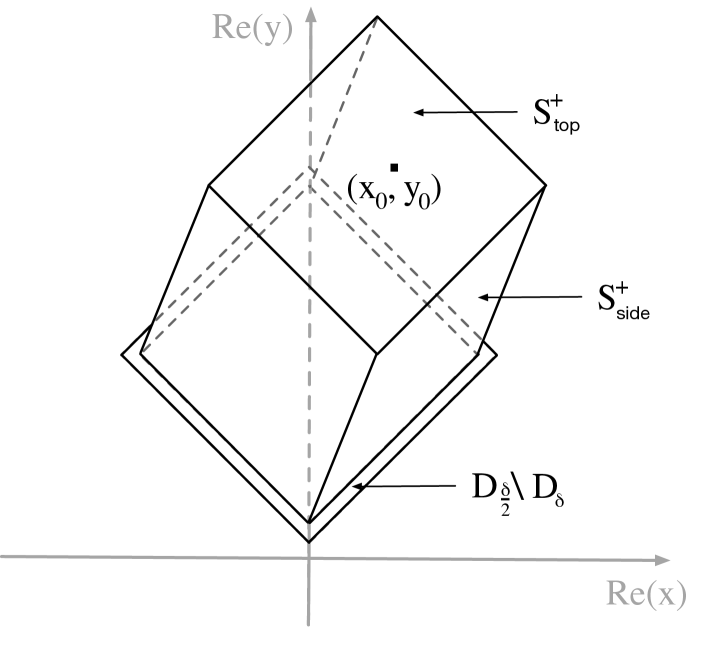
Proposition 7.2.

On $S^{+},$ $\mathrm{Im}V^{+}$ achieves the only absolute maximum at $(x_{0},y_{0});$ and on $S^{-},$ $\mathrm{Im}V^{-}$ achieves the only absolute maximum at $(-x_{0},y_{0}).$

Proof.

By Lemma 6.4, $\mathrm{Im}V^{\pm}$ is concave down on $S^{\pm}_{\text{top}}.$ Since $(\pm x_{0},y_{0})$ are respectively the critical points of $\mathrm{Im}V^{\pm},$ they are respectively the only absolute maximum on $S^{\pm}_{\text{top}}.$

On the side $S^{\pm}_{\text{side}},$ for each $(\theta_{1},\theta_{2})\in\partial D_{\delta}$ respectively consider the functions

g^{\pm}_{(\theta_{1},\theta_{2})}(t)\doteq\mathrm{Im}V^{\pm}(\theta_{1}\pm it\mathrm{Im}(x_{0}),\theta_{2}+it\mathrm{Im}(y_{0}))

on $[0,1].$ We show that $g^{\pm}_{(\theta_{1},\theta_{2})}(t)<\mathrm{Im}V^{\pm}(\pm x_{0},y_{0})$ for each $(\theta_{1},\theta_{2})\in\partial D_{\delta}$ and $t\in[0,1].$

Indeed, since $(\theta_{1},\theta_{2})\in\partial D_{\delta},$ $g^{\pm}_{(\theta_{1},\theta_{2})}(0)=\mathrm{Im}V^{\pm}(\theta_{1},\theta_{2})<\frac{1}{2}\mathrm{Vol}(\mathrm{S}^{3}{\smallsetminus}K_{4_{1}})+\epsilon<Vol(M_{K_{\theta}})=\mathrm{Im}V^{\pm}(\pm x_{0},y_{0});$ and since $(\theta_{1}\pm i\mathrm{Im}(x_{0}),\theta_{2}+i\mathrm{Im}(y_{0}))\in S^{\pm}_{\text{top}},$ by the previous step $g^{\pm}_{(\theta_{1},\theta_{2})}(1)=\mathrm{Im}V^{\pm}(\theta_{1}\pm i\mathrm{Im}(x_{0}),\theta_{2}+i\mathrm{Im}(y_{0}))<\mathrm{Im}V^{\pm}(\pm x_{0},y_{0}).$ Now by Lemma 6.4, $g^{\pm}_{(\theta_{1},\theta_{2})}$ is concave up, and hence

g^{\pm}_{(\theta_{1},\theta_{2})}(t)\leqslant\max\Big{\{}g^{\pm}_{(\theta_{1},\theta_{2})}(0),g^{\pm}_{(\theta_{1},\theta_{2})}(1)\Big{\}}<\mathrm{Im}V^{\pm}(\pm x_{0},y_{0}).

By Proposition 4.2 and assumption of $\theta,$ on $D_{\frac{\delta}{2}}{\smallsetminus}D_{\delta},$ $\mathrm{Im}V(x,y)\leqslant\frac{1}{2}\mathrm{Vol}(\mathrm{S}^{3}{\smallsetminus}K_{4_{1}})+\epsilon<\mathrm{Vol(M_{K_{\theta}})}=\mathrm{Im}V^{\pm}(\pm x_{0},y_{0}).$ ∎

Proposition 7.3.

\begin{split}\int_{D_{\frac{\delta}{2}}}\epsilon(x,y)e^{-xi+\frac{r}{4\pi i}V_{r}^{\pm}(x,y)}dxdy=\frac{4\pi}{r}\frac{e^{\frac{r}{4\pi}\Big{(}\mathrm{Vol}(M_{K_{\theta}})+i\mathrm{CS}(M_{K_{\theta}})\Big{)}}}{\sqrt{-\mathrm{Hess}V^{+}(x_{0},y_{0})}}\Big{(}1+O\Big{(}\frac{1}{r}\Big{)}\Big{)}.\end{split}

Proof.

By analyticity, the integrals remain the same if we deform the domains from $D_{\frac{\delta}{2}}$ to $S^{\pm}.$ Then by Corollary 6.2, $(\pm x_{0},y_{0})$ are respectively the critical points of $V^{\pm}.$ By Proposition 7.2, $\mathrm{Im}V^{\pm}$ achieves the only absolute maximum on $S^{\pm}$ at $(\pm x_{0},y_{0}).$ By Proposition 6.3, (2), $\mathrm{Hess}V^{\pm}(\pm x_{0},y)\neq 0.$ Finally, to estimate the difference between $V^{\pm}_{r}$ and $V^{\pm},$ we have

\varphi_{r}\Big{(}\pi-x-y-\frac{\pi}{r}\Big{)}=\varphi_{r}(\pi-x-y)-\varphi^{\prime}_{r}(\pi-x-y)\cdot\frac{\pi}{r}+O\Big{(}\frac{1}{r^{2}}\Big{)}

and

\varphi_{r}\Big{(}y-x+\frac{\pi}{r}\Big{)}=\varphi_{r}(y-x)+\varphi^{\prime}_{r}(y-x)\cdot\frac{\pi}{r}+O\Big{(}\frac{1}{r^{2}}\Big{)}.

Then by Lemma 2.6, in $\big{\{}(x,y)\in\overline{D_{\mathbb{C},\delta}}\ \big{|}\ |\mathrm{Im}x|<L,|\mathrm{Im}x|<L\}$ for some sufficiently large $L,$

V^{\pm}_{r}(x,y)=V^{\pm}(x,y)-\frac{2\pi i\big{(}\log\big{(}1-e^{-2i(y+x)}\big{)}+\log\big{(}1-e^{2i(y-x)}\big{)}\big{)}}{r}+\frac{\upsilon_{r}(x,y)}{r^{2}}

with $|\upsilon_{r}(x,y)|$ bounded from above by a constant independent of $r,$ and

e^{-xi+\frac{r}{4\pi i}V_{r}^{\pm}(x,y)}=e^{-xi-\frac{\log\big{(}1-e^{-2i(y+x)}\big{)}}{2}-\frac{\log\big{(}1-e^{2i(y-x)}\big{)}}{2}+\frac{r}{4\pi i}\Big{(}V^{\pm}(x,y)+\frac{\upsilon_{r}(x,y)}{r^{2}}\Big{)}}.

Now let $D_{\mathbf{z}}=\big{\{}(x,y)\in\overline{D_{\mathbb{C},\delta}}\ \big{|}\ |\mathrm{Im}x|<L,|\mathrm{Im}x|<L\}$ for some sufficiently large $L,$ $\mathbf{a}_{r}=\theta=\Big{|}2\pi-\frac{4\pi}{r}-\frac{4\pi m_{0}}{r}\Big{|},$ $f_{r}^{\mathbf{a}_{r}}(x,y)=V_{r}^{\pm}(x,y),$ $g_{r}^{\mathbf{a}_{r}}(x,y)=e^{-xi-\frac{\log\big{(}1-e^{-2i(y+x)}\big{)}}{2}-\frac{\log\big{(}1-e^{2i(y-x)}\big{)}}{2}},$ $f^{\mathbf{a}_{r}}(x,y)=V^{\pm}(x,y).$ Then all the conditions of Proposition 7.1 are satisfied. By the first equation of (6.2), at the critical points $(\pm x_{0},y_{0}),$

-xi-\frac{\log\big{(}1-e^{-2i(y+x)}\big{)}}{2}-\frac{\log\big{(}1-e^{2i(y-x)}\big{)}}{2}=0,

and hence $g_{r}^{\mathbf{a}_{r}}(\pm x_{0},y_{0})=1.$ By Proposition 6.3, (1), the critical values

V^{\pm}(\pm x_{0},y_{0})=i\big{(}\mathrm{Vol}(M_{K_{\theta}})+i\mathrm{CS}(M_{K_{\theta}})\big{)}

and the result follows. ∎

7.2 Estimates of other Fourier coefficients

Let

V^{(k_{0},k_{1},k_{2}),\pm}(x,y)=V^{\pm}(x,y)-\frac{4k_{0}\pi x}{q}-4k_{1}\pi x-4k_{2}\pi y,

and

\hat{F}^{\pm}(k_{0},k_{1},k_{2})=\int_{\mathcal{D}_{\frac{\delta}{2}}}e^{\frac{r}{4\pi i}V^{(k_{0},k_{1},k_{2}),\pm}(x,y)}dxdy.

By Lemma 2.6, the asymptotics of $\hat{F}^{\pm}_{r}(k_{0},k_{1},k_{2})$ is approximated by that of $\hat{F}^{\pm}(k_{0},k_{1},k_{2}).$ We will then estimate the contribution to $\hat{F}^{\pm}(k_{0},k_{1},k_{2})$ of each individual square $D_{\frac{\delta}{2}},$ $D^{\prime}_{\frac{\delta}{2}}$ and $D_{\frac{\delta}{2}}^{\prime\prime}.$

7.2.1 Estimate on $D_{\frac{\delta}{2}}$

Let

\hat{F}^{\pm}_{D}(k_{0},k_{1},k_{2})=\int_{D_{\frac{\delta}{2}}}e^{\frac{r}{4\pi i}V^{(k_{0},k_{1},k_{2}),\pm}(x,y)}dxdy.

Lemma 7.4.

For $k_{2}\neq 0,$

\hat{F}^{\pm}_{D}(k_{0},k_{1},k_{2})=O\Big{(}e^{\frac{r}{4\pi}\big{(}\mathrm{Vol}(M_{K_{\theta}})-\epsilon\big{)}}\Big{)}.

Proof.

In $D_{\mathbb{C}},$ we have

0<\arg(1-e^{-2i(y+x)})<\pi-2(\mathrm{Re}(y)+\mathrm{Re}(x))

and

2(\mathrm{Re}(y)-\mathrm{Re}(x))-\pi<\arg(1-e^{2i(y-x)})<0.

For $k_{2}>0,$ let $y=\mathrm{Re}(y)+il.$ Then

\begin{split}\frac{\partial\mathrm{Im}V^{(k_{0},k_{1},k_{2})}}{\partial l}&=4\mathrm{Re}(x)+2\arg(1-e^{-2i(y+x)})+2\arg(1-e^{2i(y-x)})-4k_{2}\pi\\ &<4x+2(\pi-2(\mathrm{Re}(y)+\mathrm{Re}(x)))+0-4k_{2}\pi\\ &=2\pi-4\mathrm{Re}(y)-4k_{2}\pi<-2\pi,\end{split}

where the last inequality comes from that $0<\mathrm{Re}(y)<\frac{\pi}{2}$ and $k_{2}>0.$ Therefore, pushing the integral domain along the $il$ direction far enough (without changing $\mathrm{Im}(x)$ ), the imaginary part of $\mathrm{Im}V^{(k_{0},k_{1},k_{2}),\pm}$ becomes smaller than the volume. Since $\mathrm{Im}V^{(k_{0},k_{1},k_{2}),\pm}$ is already smaller than the volume of $M_{K_{\theta}}$ on $\partial D_{\delta},$ it becomes even smaller on the side.

For $k_{2}<0,$ let $y=\mathrm{Re}(y)-il.$ Then

\begin{split}\frac{\partial\mathrm{Im}V^{(k_{0},k_{1},k_{2}),\pm}}{\partial l}&=-4\mathrm{Re}(x)-2\arg(1-e^{-2i(y+x)})-2\arg(1-e^{2i(y-x)})+4k_{2}\pi\\ &<-4x-0-2(2(\mathrm{Re}(y)-\mathrm{Re}(x))-\pi)+4k_{2}\pi\\ &=2\pi-4\mathrm{Re}(y)+4k_{2}\pi<-2\pi,\end{split}

where the last inequality comes from that $0<\mathrm{Re}(y)<\frac{\pi}{2}$ again and $k_{2}<0.$ Therefore, pushing the integral domain along the $-il$ direction far enough (without changing $\mathrm{Im}(x)$ ), the imaginary part of $\mathrm{Im}V^{(k_{0},k_{1},k_{2}),\pm}$ becomes smaller than the volume of $M_{K_{\theta}}.$ Since $\mathrm{Im}V^{(k_{0},k_{1},k_{2}),\pm}$ is already smaller than the volume of $M_{K_{\theta}}$ on $\partial D_{\delta},$ it becomes even smaller on the side. ∎

Lemma 7.5.

For $(k_{0},k_{1})$ so that $\frac{k_{0}}{q}+k_{1}\neq 0,$

\hat{F}^{\pm}_{D}(k_{0},k_{1},0)=O\Big{(}e^{\frac{r}{4\pi}\big{(}\mathrm{Vol}(M_{K_{\theta}})-\epsilon\big{)}}\Big{)}.

Proof.

Here we recall that $S^{\pm}=S^{\pm}_{\text{top}}\cup S^{\pm}_{\text{side}}\cup(D_{\frac{\delta}{2}}{\smallsetminus}D_{\delta}),$ where

S^{\pm}_{\text{top}}=\Big{\{}(x,y)\in D_{\mathbb{C},\delta}\ |\ (\mathrm{Im}(x),\mathrm{Im}(y))=(\pm\mathrm{Im}(x_{0}),\mathrm{Im}(y_{0}))\Big{\}}

and

S^{\pm}_{\text{side}}=\Big{\{}(\theta_{1}\pm it\mathrm{Im}(x_{0}),\theta_{2}+it\mathrm{Im}(y_{0}))\ |\ (\theta_{1},\theta_{2})\in\partial D_{\delta},t\in[0,1]\Big{\}}.

By Proposition 7.2, for any $(x,y)\in S^{\pm}_{\text{top}}$ we respectively have

\mathrm{Im}V^{\pm}(x,y)\leqslant\mathrm{Im}V^{\pm}(\pm x_{0},y_{0})=\mathrm{Vol}(M_{K_{\theta}}).

By Lemma 6.5, $\mathrm{Im}(x_{0})\neq 0.$ We first consider the case that $\mathrm{Im}(x_{0})>0.$ If $\frac{k_{0}}{q}+k_{1}>0,$ then on $S^{+}_{\text{top}}$ we have

\begin{split}\mathrm{Im}V^{(k_{0},k_{1},0),+}(x,y)=&\mathrm{Im}V^{+}(x,y)-\frac{4k_{0}\pi}{q}\mathrm{Im}(x_{0})-4k_{1}\pi\mathrm{Im}(x_{0})\\ <&\mathrm{Im}V^{+}(x,y)\leqslant\mathrm{Vol}(M_{K_{\theta}}),\end{split}

and

\begin{split}\mathrm{Im}V^{(k_{0},k_{1},0),-}(x,y)=&\mathrm{Im}V^{(k_{0},k_{1},0),+}(x,y)-\frac{2\theta}{q}\mathrm{Im}(x_{0})\\ =&\mathrm{Im}V^{+}(x,y)-\frac{2\theta}{q}\mathrm{Im}(x_{0})-\frac{4k_{0}\pi}{q}\mathrm{Im}(x_{0})-4k_{1}\pi\mathrm{Im}(x_{0})\\ <&\mathrm{Im}V^{+}(x,y)\leqslant\mathrm{Vol}(M_{K_{\theta}}).\end{split}

If $\frac{k_{0}}{q}+k_{1}<0,$ then on $S^{-}_{\text{top}}$ we have

\begin{split}\mathrm{Im}V^{(k_{0},k_{1},0),+}(x,y)=&\mathrm{Im}V^{(k_{0},k_{1},0),-}(x,y)-\frac{2\theta}{q}\mathrm{Im}(x_{0})\\ =&\mathrm{Im}V^{-}(x,y)-\frac{2\theta}{q}\mathrm{Im}(x_{0})+\frac{4k_{0}\pi}{q}\mathrm{Im}(x_{0})+4k_{1}\pi\mathrm{Im}(x_{0})\\ <&\mathrm{Im}V^{-}(x,y)\leqslant\mathrm{Vol}(M_{K_{\theta}}),\end{split}

and

\begin{split}\mathrm{Im}V^{(k_{0},k_{1},0),-}(x,y)=&\mathrm{Im}V^{-}(x,y)+\frac{4k_{0}\pi}{q}\mathrm{Im}(x_{0})+4k_{1}\pi\mathrm{Im}(x_{0})\\ <&\mathrm{Im}V^{-}(x,y)\leqslant\mathrm{Vol}(M_{K_{\theta}}).\end{split}

Next we consider the case that $\mathrm{Im}(x_{0})<0.$ Due to the fact that $k_{0}$ and $k_{1}$ are integers and $\theta\in(0,2\pi),$ if $\frac{k_{0}}{q}+k_{1}>0,$ then we have $\frac{k_{0}}{q}+k_{1}\geqslant\frac{1}{q}$ and

\frac{4\pi k_{0}}{q}+4\pi k_{1}-\frac{2\theta}{q}>0;

(7.1)

and if $\frac{k_{0}}{q}+k_{1}<0,$ then we have $\frac{k_{0}}{q}+k_{1}\leqslant-\frac{1}{q}$ and

\frac{4\pi k_{0}}{q}+4\pi k_{1}+\frac{2\theta}{q}<0.

(7.2)

Now for $(k_{0},k_{1})$ such that $\frac{k_{0}}{q}+k_{1}>0,$ we have on $S^{-}_{\text{top}}$ that

\begin{split}\mathrm{Im}V^{(k_{0},k_{1},0),+}(x,y)=&\mathrm{Im}V^{(k_{0},k_{1},0),-}(x,y)-\frac{2\theta}{q}\mathrm{Im}(x_{0})\\ =&\mathrm{Im}V^{-}(x,y)-\frac{2\theta}{q}\mathrm{Im}(x_{0})+\frac{4k_{0}\pi}{q}\mathrm{Im}(x_{0})+4k_{1}\pi\mathrm{Im}(x_{0})\\ <&\mathrm{Im}V^{-}(x,y)\leqslant\mathrm{Vol}(M_{K_{\theta}}),\end{split}

where the penultimate inequality comes from (7.1), and

\begin{split}\mathrm{Im}V^{(k_{0},k_{1},0),-}(x,y)=&\mathrm{Im}V^{-}(x,y)+\frac{4k_{0}\pi}{q}\mathrm{Im}(x_{0})+4k_{1}\pi\mathrm{Im}(x_{0})\\ <&\mathrm{Im}V^{-}(x,y)\leqslant\mathrm{Vol}(M_{K_{\theta}}).\end{split}

For $(k_{0},k_{1})$ such that $\frac{k_{0}}{q}+k_{1}<0,$ we have on $S^{+}_{\text{top}}$ that

\begin{split}\mathrm{Im}V^{(k_{0},k_{1},0),+}(x,y)=&\mathrm{Im}V^{+}(x,y)-\frac{4k_{0}\pi}{q}\mathrm{Im}(x_{0})-4k_{1}\pi\mathrm{Im}(x_{0})\\ <&\mathrm{Im}V^{+}(x,y)\leqslant\mathrm{Vol}(M_{K_{\theta}}),\end{split}

and

\begin{split}\mathrm{Im}V^{(k_{0},k_{1},0),-}(x,y)=&\mathrm{Im}V^{(k_{0},k_{1},0),+}(x,y)-\frac{2\theta}{q}\mathrm{Im}(x_{0})\\ =&\mathrm{Im}V^{+}(x,y)-\frac{2\theta}{q}\mathrm{Im}(x_{0})-\frac{4k_{0}\pi}{q}\mathrm{Im}(x_{0})-4k_{1}\pi\mathrm{Im}(x_{0})\\ <&\mathrm{Im}V^{+}(x,y)\leqslant\mathrm{Vol}(M_{K_{\theta}})\end{split}

where the penultimate inequality comes from (7.2).

We note that $V^{(k_{0},k_{1},k_{2}),\pm}$ differs from $V^{\pm}$ by a linear function. Therefore, for each $(\theta_{1},\theta_{2})\in\partial D_{\delta},$ the function

g^{\pm}_{(\theta_{1},\theta_{2})}(t)\doteq\mathrm{Im}V^{(k_{0},k_{1},0)}(\theta_{1}\pm it\mathrm{Im}(x_{0}),\theta_{2}+it\mathrm{Im}(y_{0}))

is concave up on $[0,1],$ and hence

g^{\pm}_{(\theta_{1},\theta_{2})}(t)\leqslant\max\Big{\{}g^{\pm}_{(\theta_{1},\theta_{2})}(0),g^{\pm}_{(\theta_{1},\theta_{2})}(1)\Big{\}}<\mathrm{Vol}(M_{K_{\theta}}).

Putting all together, we have: In the $\mathrm{Im}(x_{0})>0$ case, if $\frac{k_{0}}{q}+k_{1}>0,$ then $\mathrm{Im}V^{(k_{0},k_{1},0),\pm}(x,y)<\mathrm{Vol}(M_{K_{\theta}})$ on $S^{+},$ and if $\frac{k_{0}}{q}+k_{1}<0,$ then $\mathrm{Im}V^{(k_{0},k_{1},0),\pm}(x,y)<\mathrm{Vol}(M_{K_{\theta}})$ on $S^{-}.$ In the $\mathrm{Im}(x_{0})<0$ case, if $\frac{k_{0}}{q}+k_{1}>0,$ then $\mathrm{Im}V^{(k_{0},k_{1},0),\pm}(x,y)<\mathrm{Vol}(M_{K_{\theta}})$ on $S^{-},$ and if $\frac{k_{0}}{q}+k_{1}<0,$ then $\mathrm{Im}V^{(k_{0},k_{1},0),\pm}(x,y)<\mathrm{Vol}(M_{K_{\theta}})$ on $S^{+}.$ ∎

7.2.2 Estimate on $D_{\frac{\delta}{2}}^{\prime}$

Let

\hat{F}^{\pm}_{D^{\prime}}(k_{0},k_{1},k_{2})=\int_{D^{\prime}_{\delta}}e^{\frac{r}{4\pi i}V^{(k_{0},k_{1},k_{2}),\pm}(x,y)}dxdy.

Lemma 7.6.

For any triple $(k_{0},k_{1},k_{2}),$

\hat{F}^{\pm}_{D^{\prime}}(k_{0},k_{1},k_{2})=O\Big{(}e^{\frac{r}{4\pi}\big{(}\mathrm{Vol}(M_{K_{\theta}})-\epsilon\big{)}}\Big{)}.

Proof.

In $D^{\prime}_{\mathbb{C},\delta},$ we have

0<\arg(1-e^{-2i(y+x)})<\pi-2(\mathrm{Re}(y)+\mathrm{Re}(x))

and

2(\mathrm{Re}(y)-\mathrm{Re}(x))-3\pi<\arg(1-e^{2i(y-x)})<0.

For $k_{2}\geqslant 0,$ let $y=\mathrm{Re}(y)+il.$ Then

\begin{split}\frac{\partial\mathrm{Im}V^{(k_{0},k_{1},k_{2}),\pm}}{\partial l}&=4\mathrm{Re}(x)+2\arg(1-e^{-2i(y+x)})+2\arg(1-e^{2i(y-x)})-4k_{2}\pi\\ &<4x+2(\pi-2(\mathrm{Re}(y)+\mathrm{Re}(x)))+0-4k_{2}\pi\\ &=2\pi-4\mathrm{Re}(y)-4k_{2}\pi<-2\delta,\end{split}

where the last inequality comes from that $\frac{\pi}{2}+\frac{\delta}{2}<\mathrm{Re}(y)<\pi-\frac{\delta}{2}$ and $k_{2}\geqslant 0.$ Therefore, pushing the integral domain along the $il$ direction far enough (without changing $\mathrm{Im}(x)$ ), the imaginary part of $\mathrm{Im}V^{(k_{0},k_{1},k_{2}),\pm}$ becomes smaller than the volume of $M_{K_{\theta}}.$ Since $\mathrm{Im}V^{(k_{0},k_{1},k_{2}),\pm}$ is already smaller than the volume of $M_{K_{\theta}}$ on $\partial D^{\prime}_{\delta},$ it becomes even smaller on the side.

For $k_{2}<0,$ let $y=\mathrm{Re}(y)-il.$ Then

\begin{split}\frac{\partial\mathrm{Im}V^{(k_{0},k_{1},k_{2}),\pm}}{\partial l}&=-4\mathrm{Re}(x)-2\arg(1-e^{-2i(y+x)})-2\arg(1-e^{2i(y-x)})+4k_{2}\pi\\ &<-4x-0-2(2(\mathrm{Re}(y)-\mathrm{Re}(x))-3\pi)+4k_{2}\pi\\ &=6\pi-4\mathrm{Re}(y)+4k_{2}\pi<-2\delta,\end{split}

where the last inequality comes from that $\frac{\pi}{2}+\frac{\delta}{2}<\mathrm{Re}(y)<\pi-\frac{\delta}{2}$ again and $k_{2}<0.$ Therefore, pushing the integral domain along the $-il$ direction far enough (without changing $\mathrm{Im}(x)$ ), the imaginary part of $\mathrm{Im}V^{(k_{0},k_{1},k_{2}),\pm}$ becomes smaller than the volume of $M_{K_{\theta}}.$ Since $\mathrm{Im}V^{(k_{0},k_{1},k_{2}),\pm}$ is already smaller than the volume of $M_{K_{\theta}}$ on $\partial D^{\prime}_{\delta},$ it becomes even smaller on the side. ∎

7.2.3 Estimate on $D_{\frac{\delta}{2}}^{\prime\prime}$

Let

\hat{F}^{\pm}_{D^{\prime\prime}}(k_{0},k_{1},k_{2})=\int_{D^{\prime\prime}_{\delta}}e^{\frac{r}{4\pi i}V^{(k_{0},k_{1},k_{2}),\pm}(x,y)}dxdy.

Lemma 7.7.

For any triple $(k_{0},k_{1},k_{2}),$

\hat{F}^{\pm}_{D^{\prime\prime}}(k_{0},k_{1},k_{2})=O\Big{(}e^{\frac{r}{4\pi}\big{(}\mathrm{Vol}(M_{K_{\theta}})-\epsilon\big{)}}\Big{)}.

Proof.

In $D^{\prime\prime}_{\mathbb{C},\delta},$ we have

0<\arg(1-e^{-2i(y+x)})<3\pi-2(\mathrm{Re}(y)+\mathrm{Re}(x))

and

2(\mathrm{Re}(y)-\mathrm{Re}(x))-\pi<\arg(1-e^{2i(y-x)})<0.

For $k_{2}>0,$ let $y=\mathrm{Re}(y)+il.$ Then

\begin{split}\frac{\partial\mathrm{Im}V^{(k_{0},k_{1},k_{2}),\pm}}{\partial l}&=4\mathrm{Re}(x)+2\arg(1-e^{-2i(y+x)})+2\arg(1-e^{2i(y-x)})-4k_{2}\pi\\ &<4x+2(3\pi-2(\mathrm{Re}(y)+\mathrm{Re}(x)))+0-4k_{2}\pi\\ &=6\pi-4\mathrm{Re}(y)-4k_{2}\pi<-2\delta,\end{split}

where the last inequality comes from that $\frac{\pi}{2}+\frac{\delta}{2}<\mathrm{Re}(y)<\pi-\frac{\delta}{2}$ and $k_{2}>0.$ Therefore, pushing the integral domain along the $il$ direction far enough (without changing $\mathrm{Im}(x)$ ), the imaginary part of $\mathrm{Im}V^{(k_{0},k_{1},k_{2}),\pm}$ becomes smaller than the volume of $M_{K_{\theta}}.$ Since $\mathrm{Im}V^{(k_{0},k_{1},k_{2}),\pm}$ is already smaller than the volume of $M_{K_{\theta}}$ on $\partial D^{\prime\prime}_{\delta},$ it becomes even smaller on the side.

For $k_{2}\leqslant 0,$ let $y=\mathrm{Re}(y)-il.$ Then

\begin{split}\frac{\partial\mathrm{Im}V^{(k_{0},k_{1},k_{2}),\pm}}{\partial l}&=-4\mathrm{Re}(x)-2\arg(1-e^{-2i(y+x)})-2\arg(1-e^{2i(y-x)})+4k_{2}\pi\\ &<-4x-0-2(2(\mathrm{Re}(y)-\mathrm{Re}(x))-\pi)+4k_{2}\pi\\ &=2\pi-4\mathrm{Re}(y)+4k_{2}\pi<-2\delta,\end{split}

where the last inequality comes from that $\frac{\pi}{2}+\frac{\delta}{2}<\mathrm{Re}(y)<\pi-\frac{\delta}{2}$ again and $k_{2}\leqslant 0.$ Therefore, pushing the integral domain along the $-il$ direction far enough (without changing $\mathrm{Im}(x)$ ), the imaginary part of $\mathrm{Im}V^{(k_{0},k_{1},k_{2}),\pm}$ becomes smaller than the volume of $M_{K_{\theta}}.$ Since $\mathrm{Im}V^{(k_{0},k_{1},k_{2}),\pm}$ is already smaller than the volume of $M_{K_{\theta}}$ on $\partial D^{\prime\prime}_{\delta},$ it becomes even smaller on the side.∎

7.3 Proof of Theorem 1.2

Theorem 1.2 follows from the following proposition.

Proposition 7.8.

(1)

\begin{split}\hat{f}^{+}_{r}(0,\dots,0)+&\hat{f}^{-}_{r}(,0,\dots,0)=\frac{-2i^{-\frac{k-3}{2}}r^{\frac{k+1}{2}}}{\pi\sqrt{q}\sqrt{-\mathrm{Hess}V^{+}(x_{0},y_{0})}}e^{\frac{r}{4\pi}\big{(}\mathrm{Vol}(M_{K_{\theta}})+i\mathrm{CS}(M_{K_{\theta}})\big{)}}\Big{(}1+O\Big{(}\frac{1}{\sqrt{r}}\Big{)}\Big{)}.\end{split}

(2)

For $(n_{1},\dots,n_{k-1},k_{1},k_{2})\neq(0,\dots,0),$

\begin{split}|\hat{f}^{\pm}_{r}(n_{1},\dots,n_{k-1},k_{1},k_{2})|\leqslant O\Big{(}r^{\frac{k}{2}}\Big{)}e^{\frac{r}{4\pi}\mathrm{Vol}(M_{K_{\theta}})}.\end{split}

Proof.

By Lemmas 7.6 and 7.7, the contribution of $D^{\prime}_{\frac{\delta}{2}}$ and $D^{\prime\prime}_{\frac{\delta}{2}}$ to $\hat{f}_{r}(n_{1},\dots,n_{k-1},k_{1},k_{2})$ is of order $O\big{(}e^{\frac{r}{4\pi}\big{(}\mathrm{Vol}(M_{K_{\theta}})-\epsilon\big{)}}\big{)},$ hence is neglectable.

Then (1) follows from Propositions 5.4 and 7.3.

To see (2), for $(n_{1},\dots,n_{k-1},k_{1},k_{2})\neq(0,\dots,0)$ with $\big{(}\frac{k_{0}}{q}+k_{1},k_{2}\big{)}\neq(0,0),$ by Proposition 5.7 (1), Lemmas 7.4 and 7.5, and Lemma 2.6, we have that

\hat{f}^{\pm}_{r}(n_{1},n_{2},\dots,n_{k-1},k_{1},k_{2})=O\Big{(}e^{\frac{r}{4\pi}\big{(}\mathrm{Vol}(M_{K_{\theta}})-\epsilon\big{)}}\Big{)}.

If $\big{(}\frac{k_{0}}{q}+k_{1},k_{2}\big{)}=(0,0),$ in particular, if $\frac{k_{0}}{q}+k_{1}=0,$ then $|k_{0}|=|qk_{1}|$ is either $0$ or greater than or equal to $q.$ Then by Propositions 5.7 (2) and 7.3, and Lemma 2.6,

|\hat{f}^{\pm}_{r}(n_{1},n_{2},\dots,n_{k-1},k_{1},k_{2})|\leqslant O\Big{(}r^{\frac{k}{2}}\Big{)}e^{\frac{r}{4\pi}\mathrm{Vol}(M_{K_{\theta}})}.

∎

Proof of Theorem 1.2.

By Propositions 4.1 and 7.8, we have

\begin{split}&\lim_{r\to\infty}\frac{4\pi}{r}\log\mathrm{RT}_{r}(M_{K_{\theta}})\\ =&\lim_{r\to\infty}\frac{4\pi}{r}\bigg{(}\log\kappa_{r}+\log\bigg{(}\sum\hat{f}^{\pm}_{r}(n_{1},\dots,n_{k-1},k_{1},k_{2})+O\Big{(}e^{\frac{r}{4\pi}\big{(}\frac{1}{2}\mathrm{Vol}(\mathrm{S}^{3}{\smallsetminus}K_{4_{1}})+\epsilon\big{)}}\Big{)}\bigg{)}\bigg{)}\\ =&i\Big{(}3\sum_{i=1}^{k}a_{i}+\sigma(L)+2k-2\Big{)}\pi^{2}+\mathrm{Vol}(M_{K_{\theta}})+i\mathrm{CS}(M_{K_{\theta}})\\ =&\mathrm{Vol}(M_{K_{\theta}})+i\mathrm{CS}(M_{K_{\theta}})\quad\text{mod }i\pi^{2}\mathbb{Z}.\end{split}

∎

7.4 Cone angles satisfying the assumption of Theorem 1.2

Proposition 7.9.

(1)

If $(p,q)\neq(\pm 1,0),$ $(0,\pm 1),$ $(\pm 1,\pm 1),$ $(\pm 2,\pm 1),$ $(\pm 3,\pm 1),$ $(\pm 4,\pm 1)$ and $(\pm 5,\pm 1),$ then for any cone angle $\theta$ less than or equal to $2\pi,$

$\mathrm{Vol}(M_{K_{\theta}})>\frac{\mathrm{Vol}(S^{3}{\smallsetminus}K_{4_{1}})}{2}.$
(2)

If $(p,q)=(0,\pm 1),$ $(\pm 1,\pm 1),$ $(\pm 2,\pm 1),$ $(\pm 3,\pm 1),$ $(\pm 4,\pm 1)$ or $(\pm 5,\pm 1),$ then for any cone angle $\theta$ less than or equal to $\pi,$

$\mathrm{Vol}(M_{K_{\theta}})>\frac{\mathrm{Vol}(S^{3}{\smallsetminus}K_{4_{1}})}{2}.$

Proof.

By [28, Proposition 7.2], (1) holds for $\theta=2\pi.$ Then by [12, Corollary 5.4] that $\mathrm{Vol}(M_{K_{\theta}})$ is decreasing in $\theta,$ (1) holds for all $\theta$ less than $2\pi.$

For (2), by [12, Chapter 6] have that for $(p,q)=(0,\pm 1),$ $(\pm 1,\pm 1),$ $(\pm 2,\pm 1),$ $(\pm 3,\pm 1),$ $(\pm 4,\pm 1)$ or $(\pm 5,\pm 1)$ and for any $\theta$ less than $2\pi$ there exists a unique hyperbolic cone metric on $M$ with singular locus $K$ with cone angle $\theta,$ with $\mathrm{Vol}(M_{K_{0}})=\mathrm{Vol}(S^{3}{\smallsetminus}K_{4_{1}})$ and $\mathrm{Vol}(M_{K_{2\pi}})=\mathrm{Vol}(M)\geqslant 0.$ Let $L_{\theta}$ be the length of $K$ in $M_{K_{\theta}}.$ Then by the Schläfli formula [12, Theorem 5.2],

\frac{d^{2}\mathrm{Vol}(M_{K_{\theta}})}{d\theta^{2}}=-\frac{dL_{\theta}}{d\theta}.

Let $m$ and $l$ respectively be the meridian and longitude of the boundary of the figure-8 complement as in Section 6, then $m$ is isotopic to $K$ in $M,$ and

\left\{\begin{array}[]{c}p\mathrm{H}(m)+\mathrm{H}(l)=\theta i\\ \\ \mathrm{H}(m)=L_{\theta}.\end{array}\right.

As a consequence, we have

p+\frac{d\mathrm{H}(l)}{dL_{\theta}}=i\frac{d\theta}{dL_{\theta}},

and hence

\frac{dL_{\theta}}{d\theta}=\bigg{(}\mathrm{Im}\frac{d\mathrm{H}(l)}{d\mathrm{H}(m)}\bigg{)}^{-1}.

By [20, Formula (68)], we have

\frac{d\mathrm{H}(l)}{d\mathrm{H}(m)}=2\frac{1-2e^{L_{\theta}}-2e^{-L_{\theta}}}{\sqrt{e^{2L_{\theta}}+e^{-2L_{\theta}}-2e^{L_{\theta}}-2e^{-L_{\theta}}+1}},

which implies that $\mathrm{Im}\frac{d\mathrm{H}(l)}{d\mathrm{H}(m)}>0,$ and hence $\frac{dL_{\theta}}{d\theta}>0$ and $\frac{d^{2}\mathrm{Vol}(M_{K_{\theta}})}{d\theta^{2}}=-\frac{dL_{\theta}}{d\theta}<0.$ As a consequence, $\mathrm{Vol}(M_{K_{\theta}})$ is strictly concave down in $\theta,$ and

\mathrm{Vol}(M_{K_{\pi}})>\frac{\mathrm{Vol}(M_{K_{0}})+\mathrm{Vol}(M_{K_{2\pi}})}{2}\geqslant\frac{\mathrm{Vol}(S^{3}{\smallsetminus}K_{4_{1}})}{2}.

Then by the monotonicity,

\mathrm{Vol}(M_{K_{\theta}})>\frac{\mathrm{Vol}(S^{3}{\smallsetminus}K_{4_{1}})}{2}

for all cone angle $\theta$ less than or equal to $\pi.$ ∎

Remark 7.10.

We note that the upper bound $\pi$ in (2) of Proposition 7.9 is not sharp.

References

[1] G. Belletti, R. Detcherry, E. Kalfagianni, and T. Yang, Growth of quantum 6j-symbols and applications to the Volume Conjecture, to appear in J. Differential Geom.
[2] C. Blanchet, N. Habegger, G. Masbaum and P. Vogel, Three-manifold invariants derived from the Kauffman bracket, Topology 31 (1992), no. 4, 685–699.
[3] Q. Chen and J. Murakami, Asymptotics of quantum $6j$ symbols, preprint, arXiv:1706.04887.
[4] Q. Chen and T. Yang, Volume Conjectures for the Reshetikhin-Turaev and the Turaev-Viro Invariants, Quantum Topol. 9 (2018), no. 3, 419–460.
[5] D. Cooper, C. Hodgson and S. Kerckhoff, Three-dimensional orbifolds and cone-manifolds. With a postface by Sadayoshi Kojima, MSJ Memoirs, 5. Mathematical Society of Japan, Tokyo, 2000. x+170 pp. ISBN: 4-931469-05-1.
[6] R. Detcherry and E. Kalfagianni, Gromov norm and Turaev-Viro invariants of 3-manifolds, to appear in Ann. Sci. de l’Ecole Normale Sup..
[7] R. Detcherry, E. Kalfagianni and T. Yang, Turaev-Viro invariants, colored Jones polynomials and volume, Quantum Topol. 9 (2018), no. 4, 775–813.
[8] L. Faddeev, Discrete Heisenberg-Weyl group and modular group, Lett. Math. Phys. 34 (1995), no. 3, 249–254.
[9] L. Faddeev, R. Kashaev and A. Volkov, Strongly coupled quantum discrete Liouville theory, I. Algebraic approach and duality. Comm. Math. Phys. 219 (2001), no. 1, 199–219.
[10] S. Garoufalidis and T. Le, Asymptotics of the colored Jones function of a knot, Geom. Topol. 15 (2011), no. 4, 2135–2180.
[11] K. Habiro. On the colored Jones polynomial of some simple links, In: Recent Progress Towards the Volume Conjecture, Research Institute for Mathematical Sciences (RIMS) Kokyuroku 1172, September 2000.
[12] C. Hodgson, Degeneration and regeneration of geometric structures on three-manifolds (foliations, Dehn surgery), Thesis (Ph.D.) Princeton University. 1986. 175 pp.
[13] C. Hodgson and S. Kerckhoff, Rigidity of hyperbolic cone-manifolds and hyperbolic Dehn surgery, J. Differential Geom. 48 (1998) 1–59.
[14] R. Kashaev, A link invariant from quantum dilogarithm, Modern Phys. Lett. A 10 (1995), no. 19, 1409–1418.
[15] R. Kashaev, The hyperbolic volume of knots from the quantum dilogarithm, Lett. Math. Phys. 39 (1997), no. 3, 269–275.
[16] S. Kojima, Deformations of hyperbolic 3-cone-manifolds, J. Differential Geom. 49 (1998), no. 3, 469–516.
[17] D. London, A note on matrices with positive definite real part, Proc. Amer. Math. Soc. 82 (1981), no. 3, 322–324.
[18] W. Lickorish, The skein method for three-manifold invariants, J. Knot Theory Ramifications 2 (1993), no. 2, 171–194.
[19] G. Masbaum Skein-theoretical derivation of some formulas of Habiro, Algebr. Geom. Topol., 3, no. 1 (2003), 537–556.
[20] W. Neumann and D. Zagier, Volumes of hyperbolic three-manifolds, Topology 24 (1985), no. 3, 307– 332.
[21] T. Ohtsuki, On the asymptotic expansion of the Kashaev invariant of the $5_{2}$ knot, Quantum Topol. 7 (2016), no. 4, 669 –735.
[22] T. Ohtsuki, On the asymptotic expansion of the quantum $SU(2)$ invariant at $q=\exp(4\pi\sqrt{-1}/N)$ for closed hyperbolic 3-manifolds obtained by integral surgery along the figure-eight knot, Algebr. Geom. Topol. 18 (2018), no. 7, 4187–4274.
[23] N. Reshetikhin and V. Turaev, Ribbon graphs and their invariants derived from quantum groups, Comm. Math. Phys. 127 (1990), no. 1, 1–26.
[24] N. Reshetikhin and V. Turaev, Invariants of $3$ -manifolds via link polynomials and quantum groups, Invent. Math. 103 (1991), no. 3, 547–597.
[25] D. Rolfsen, Knots and links, 2nd printing with corrections, Mathematics Lecture Series 7, Publish or Perish, Inc. (1990).
[26] E. Stein and R. Shakarchi, Fourier analysis, An introduction. Princeton Lectures in Analysis, 1. Princeton University Press, Princeton, NJ, 2003. xvi+311 pp. ISBN: 0-691-11384-X.
[27] W. Thurston, The geometry and topology of $3$ -manifolds, Princeton Univ. Math. Dept. (1978). Available from http://msri.org/publications/books/gt3m/.
[28] K. H. Wong and T. Yang, On the Volume Conjecture for hyperbolic Dehn-filled $3$ -manifolds along the figure-eight knot, arXiv:2003.10053.
[29] K. H. Wong and T. Yang, Relative Reshetikhin-Turaev invariants, hyperbolic cone metrics and discrete Fourier transforms I, arXiv: 2008.05045.
[30] E. Witten, Quantum field theory and the Jones polynomial, Comm. Math. Phys. 121 (3): 351–399.
[31] T. Yoshida, The $\eta$ -invariant of hyperbolic $3$ -manifolds, Invent. Math. 81 (1985), no. 3, 473–514.
[32] D. Zagier, The dilogarithm function, Frontiers in number theory, physics, and geometry. II, 3–65, Springer, Berlin, 2007.

Ka Ho Wong
Department of Mathematics
Texas A&M University
College Station, TX 77843, USA
(daydreamkaho@math.tamu.edu)

Tian Yang
Department of Mathematics
Texas A&M University
College Station, TX 77843, USA
(tianyang@math.tamu.edu)

Relative Reshetikhin-Turaev invariants, hyperbolic cone metrics and discrete Fourier transforms II

Abstract

1 Introduction

Conjecture 1.1 ([29]).

Theorem 1.2.

2 Preliminaries

2.1 Relative Reshetikhin-Turaev invariants

2.2 Hyperbolic cone manifolds

Definition 2.1.

Remark 2.2.

2.3 Dilogarithm and Lobachevsky functions

2.4 Quantum dilogarithm functions

Lemma 2.3.

Lemma 2.4.

Lemma 2.5.

Lemma 2.6.

3 Computation of the relative Reshetikhin-Turaev invariants

Proposition 3.1.

Proof.

4 Poisson summation formula

Proposition 4.1.

Proof.

Proposition 4.2.

Lemma 4.3.

Proof of Proposition 4.2.

5 A simplification of the Fourier coefficients

Lemma 5.1.

Lemma 5.2.

Lemma 5.3.

Proof.

Proposition 5.4.

Proof.

Proposition 5.5.

Lemma 5.6.

Proof.

Proposition 5.7.

6 Geometry of the critical points

Lemma 6.1.

Proof.

Corollary 6.2.

Proposition 6.3.

Proof.

Lemma 6.4.

Proof.

Lemma 6.5.

Proof.

7 Asymptotics

7.1 Asymptotics of the leading Fourier coefficients

Proposition 7.1.

Proposition 7.2.

Proof.

Proposition 7.3.

Proof.

7.2 Estimates of other Fourier coefficients

7.2.1 Estimate on Dδ2D_{\frac{\delta}{2}}

Lemma 7.4.

Proof.

Lemma 7.5.

Proof.

7.2.2 Estimate on Dδ2′D_{\frac{\delta}{2}}^{\prime}

Lemma 7.6.

Proof.

7.2.3 Estimate on Dδ2′′D_{\frac{\delta}{2}}^{\prime\prime}

Lemma 7.7.

Proof.

7.3 Proof of Theorem 1.2

Proposition 7.8.

Proof.

Proof of Theorem 1.2.

7.4 Cone angles satisfying the assumption of Theorem 1.2

Proposition 7.9.

Proof.

Remark 7.10.

References

7.2.1 Estimate on $D_{\frac{\delta}{2}}$

7.2.2 Estimate on $D_{\frac{\delta}{2}}^{\prime}$

7.2.3 Estimate on $D_{\frac{\delta}{2}}^{\prime\prime}$