This paper was converted on www.awesomepapers.org from LaTeX by an anonymous user.
Want to know more? Visit the Converter page.

Relativistic spin dynamics for vector mesons

Xin-Li Sheng Key Laboratory of Quark and Lepton Physics (MOE) and Institute of Particle Physics, Central China Normal University, Wuhan, 430079,China    Lucia Oliva Department of Physics and Astronomy "Ettore Majorana", University of Catania, Via S. Sofia 64, I-95123 Catania, Italy INFN Sezione di Catania, Via S. Sofia 64, I-95123 Catania, Italy    Zuo-Tang Liang Key Laboratory of Particle Physics and Particle Irradiation (MOE), Institute of Frontier and Interdisciplinary Science, Shandong University, Qingdao, Shandong 266237, China    Qun Wang Peng Huanwu Center for Fundamental Theory and Department of Modern Physics, University of Science and Technology of China, Hefei, Anhui 230026, China    Xin-Nian Wang Nuclear Science Division, MS 70R0319, Lawrence Berkeley National Laboratory, Berkeley, California 94720, USA
Abstract

We propose a relativistic theory for spin density matrices of vector mesons based on Kadanoff-Baym equations in the closed-time-path formalism. The theory puts the calculation of spin observables such as the spin density matrix element ρ00\rho_{00} for vector mesons on a solid ground. Within the theory we formulate ρ00\rho_{00} for ϕ\phi mesons into a factorization form in separation of momentum and space-time variables. We argue that the main contribution to ρ00\rho_{00} at lower energies should be from the ϕ\phi fields that can polarize the strange quark and antiquark in the same way as electromagnetic fields. The key observation is that there is correlation inside the ϕ\phi meson wave function between the ϕ\phi field that polarizes the strange quark and that polarizes the strange antiquark. This is reflected by the fact that the contributions to ρ00\rho_{00} are all in squares of fields which are nonvanishing even if the fields may strongly fluctuate in space-time. The fluctuation of strong force fields can be extracted from ρ00\rho_{00} of quarkonium vector mesons as links to fundamental properties of quantum chromodynamics.

I Introduction

There is an intrinsic connection between rotation and spin polarization since they are related to the conservation of total angular momentum and can be converted from one to another, as demonstrated in the Barnett effect (Barnett, 1935) and the Einstein-de Haas effect (Einstein and de Haas, 1915) in materials. A recent example is the observation of a spin-current from the vortical motion in a liquid metal (Takahashi et al., 2016). The same effects also exist in high energy heavy-ion collisions (HIC) in which the huge orbital angular momentum (OAM) along the direction normal to the reaction plane can be partially converted to the global spin polarization of hadrons (Liang and Wang, 2005a, b; Voloshin, 2004; Betz et al., 2007; Becattini et al., 2008; Gao et al., 2008) (see, e.g. (Wang, 2017; Florkowski et al., 2019; Becattini and Lisa, 2020; Gao et al., 2021; Huang et al., 2020a), for recent reviews). The global spin polarization of Λ\Lambda (including Λ¯\overline{\Lambda} hereafter) has been measured through their weak decays in Au+Au collisions at sNN=7.7200\sqrt{s_{NN}}=7.7-200 GeV (Adamczyk et al., 2017; Adam et al., 2018).

As spin-one particles, vector mesons can also be polarized in heavy ion collisions in the same way as hyperons. Normally the spin states of vector mesons are described by the spin density matrix element ρλ1λ2\rho_{\lambda_{1}\lambda_{2}} with λ1,λ2=0,±1\lambda_{1},\lambda_{2}=0,\pm 1 labeling spin states along the spin quantization direction. The vector mesons mainly decay through strong interaction that respects parity symmetry. So their spin polarization proportional to ρ11ρ1,1\rho_{11}-\rho_{-1,-1} cannot be measured through their decays. Instead, ρ00\rho_{00} can be measured through the angular distribution of its decay daughters (Liang and Wang, 2005b; Yang et al., 2018; Tang et al., 2018; Gonçalves and Torrieri, 2022). If ρ00=1/3\rho_{00}=1/3, the spin states are equally populated in the three spin states implying that the vector meson is not polarized. If ρ001/3\rho_{00}\neq 1/3, the three spin states are not equally populated, so the spin of the vector meson is aligned either in the direction of the spin quantization or of the transverse direction perpendicular to it. In 2008, the STAR collaboration measured ρ00\rho_{00} for the vector meson ϕ(1020)\phi(1020) in Au+Au collisions at 200 GeV, but the result is consistent with 1/31/3 within errors due to statistics (Abelev et al., 2008). Recently STAR has measured the ϕ\phi meson’s ρ00\rho_{00} at lower energies which shows a significant deviation from 1/31/3 (Abdallah et al., 2022). It can hardly be explained by conventional mechanism (Yang et al., 2018; Xia et al., 2021; Gao, 2021; Müller and Yang, 2022). In Ref. (Sheng et al., 2020a), some of us proposed that a large deviation of ρ00\rho_{00} from 1/3 for the ϕ\phi meson may possibly arise from the ϕ\phi field, a strong force field with vacuum quantum number in connection with pseudo-Goldstone bosons and vacuum properties of quantum chromodynamics. Such a proposal is based on a nonrelativistic quark coalescence model for the spin density matrix of vector mesons (Yang et al., 2018; Sheng et al., 2020b).

In this paper we will present a relativistic theory for the spin density matrix of vector mesons from the Kadanoff-Baym (KB) equation (Kadanoff and Baym, 1962) in the closed-time-path (CTP) formalism (Martin and Schwinger, 1959; Keldysh, 1964) (for reviews of the KB equation and the CTP formalism, we refer the readers to Refs. (Chou et al., 1985; Blaizot and Iancu, 2002; Berges, 2004; Cassing, 2009)). Then we can derive the spin Boltzmann equation for vector mesons with their spin density matrices being expressed in terms of the matrix valued spin dependent distributions (MVSD) of the quarks and antiquarks (Sheng et al., 2021). This puts the calculation of spin observables such as ρ00\rho_{00} for vector mesons on a solid ground.

The paper is organized as follows. In Sec. II we will give an introduction to Green functions on the CTP for vector mesons which can be expressed in MVSD. In Sec. III the KB equations for vector mesons are derived. In Sec. IV the spin density matrices for vector mesons will be formulated from the spin Boltzmann equations. In Sec. V the spin density matrices for ϕ\phi mesons will be evaluated. Discussions on the main results and conclusions are given in the final section, Sec. VI.

We adopt the sign convention for the metric tensor gμν=gμν=diag(1,1,1,1)g^{\mu\nu}=g_{\mu\nu}=\mathrm{diag}(1,-1,-1,-1) where μ,ν=0,1,2,3\mu,\nu=0,1,2,3. The sign convention for the Levi-Civita symbol is ϵ0123=ϵ0123=1\epsilon^{0123}=-\epsilon_{0123}=1. We can write the space-time coordinate as x=xμ=(x0,𝐱)=(t,𝐱)x=x^{\mu}=(x^{0},\mathbf{x})=(t,\mathbf{x}) and xμ=(x0,𝐱)x_{\mu}=(x_{0},-\mathbf{x}) with x0=x0=tx_{0}=x^{0}=t. The four-momentum for a particle is denoted as p=pμ=(p0,𝐩)p=p^{\mu}=(p^{0},\mathbf{p}) or pμ=(p0,𝐩)p_{\mu}=(p_{0},-\mathbf{p}), if it is on-shell we have p0=p0=𝐩2+m2Ep=E𝐩p_{0}=p^{0}=\sqrt{\mathbf{p}^{2}+m^{2}}\equiv E_{p}=E_{\mathbf{p}}. Normally we use Greek letters to denote four-dimensional indices of four-vectors and four-tensors and Latin letters to denote their spatial components.

II Green functions on CTP for vector mesons

The massive spin-1 particle, such as the vector meson with the mass mVm_{V}, can be described by the vector field AVμ(x)A_{V}^{\mu}(x) with the classical Lagrangian density

=14FμνVFVμν+mV22AμVAVμAμVjμ.\mathcal{L}=-\frac{1}{4}F_{\mu\nu}^{V}F_{V}^{\mu\nu}+\frac{m_{V}^{2}}{2}A_{\mu}^{V}A_{V}^{\mu}-A_{\mu}^{V}j^{\mu}. (1)

where jμj^{\mu} is the source current, FVμν=μAVννAVμF_{V}^{\mu\nu}=\partial^{\mu}A_{V}^{\nu}-\partial^{\nu}A_{V}^{\mu} is the field strength tensor, and AVμA_{V}^{\mu} is assumed to be the real classical field for the charge (including flavor) neutral particle. From \mathcal{L} one can obtain the Proca equation (Proca, 1936; Itzykson and Zuber, 1980)

Lμν(x)AνV(x)=jμ(x),L^{\mu\nu}(x)A_{\nu}^{V}(x)=j^{\mu}(x), (2)

where the differential operator is defined as

Lμν(x)=(x2+mV2)gμνxμxν.L^{\mu\nu}(x)=\left(\partial_{x}^{2}+m_{V}^{2}\right)g^{\mu\nu}-\partial_{x}^{\mu}\partial_{x}^{\nu}. (3)

A constraint equation can be derived by contracting the above equation with μ\partial_{\mu} as

μAVμ(x)=1mV2μjμ(x)=0,\partial_{\mu}A_{V}^{\mu}(x)=\frac{1}{m_{V}^{2}}\partial_{\mu}j^{\mu}(x)=0, (4)

if the source current is conserved μjμ=0\partial_{\mu}j^{\mu}=0. The above equation means that the longitudinal component of AVμ(x)A_{V}^{\mu}(x) is vanishing for the conserved current.

The free vector field can be quantized as

AVμ(x)\displaystyle A_{V}^{\mu}(x) =\displaystyle= λ=0,±1d3k(2π)312EkV\displaystyle\sum_{\lambda=0,\pm 1}\int\frac{d^{3}k}{(2\pi\hbar)^{3}}\frac{1}{2E_{k}^{V}} (5)
×[ϵμ(λ,𝐤)aV(λ,𝐤)eikx/+ϵμ(λ,𝐤)aV(λ,𝐤)eikx/],\displaystyle\times\left[\epsilon^{\mu}(\lambda,{\bf k})a_{V}(\lambda,{\bf k})e^{-ik\cdot x/\hbar}+\epsilon^{\mu\ast}(\lambda,{\bf k})a_{V}^{\dagger}(\lambda,{\bf k})e^{ik\cdot x/\hbar}\right],

where EkV=𝐤2+mV2E_{k}^{V}=\sqrt{\mathbf{k}^{2}+m_{V}^{2}} and λ\lambda denote the energy and the spin state in the spin quantization direction respectively, the creation and annihilation operators aV(λ,𝐤)a_{V}(\lambda,{\bf k}) and aV(λ,𝐤)a_{V}^{\dagger}(\lambda,{\bf k}) satisfy the commutator

[aV(λ,𝐤),aV(λ,𝐤)]=δλλ2E𝐤(2π)3δ(3)(𝐤𝐤),\left[a_{V}(\lambda,{\bf k}),a_{V}^{\dagger}(\lambda^{\prime},{\bf k}^{\prime})\right]=\delta_{\lambda\lambda^{\prime}}2E_{{\bf k}}(2\pi\hbar)^{3}\delta^{(3)}({\bf k}-{\bf k}^{\prime}), (6)

and the polarization vector ϵμ(λ,𝐤)\epsilon^{\mu}(\lambda,{\bf k}) obeys

kμϵμ(λ,𝐤)=0,\displaystyle k_{\mu}\epsilon^{\mu}(\lambda,{\bf k})=0,
ϵ(λ,𝐤)ϵ(λ,𝐤)=δλλ,\displaystyle\epsilon(\lambda,{\bf k})\cdot\epsilon^{*}(\lambda^{\prime},{\bf k})=-\delta_{\lambda\lambda^{\prime}},
λϵμ(λ,𝐤)ϵν(λ,𝐤)=(gμνkμkνmV2).\displaystyle\sum_{\lambda}\epsilon^{\mu}(\lambda,{\bf k})\epsilon^{\nu*}(\lambda,{\bf k})=-\left(g^{\mu\nu}-\frac{k^{\mu}k^{\nu}}{m_{V}^{2}}\right). (7)

In above relations, the first one follows the constraint (4) and kμ=(EkV,𝐤)k^{\mu}=(E_{k}^{V},\mathbf{k}) denotes the on-shell four-momentum for the vector meson. By the field quantization in (5), one can check that AVμ(x)A_{V}^{\mu}(x) is Hermitian, i.e. AVμ(x)=AVμ(x)A_{V}^{\mu\dagger}(x)=A_{V}^{\mu}(x).

Refer to caption
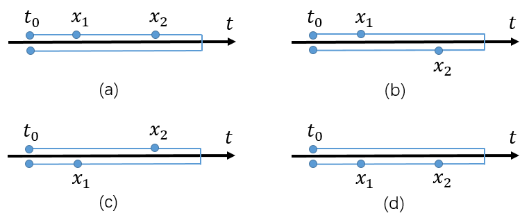
Figure 1: The closed-time path and four components of the two-point Green function on CTP. The positive and negative time-branches are denoted as C+C_{+} and CC_{-} respectively. (a) x10=t1C+x_{1}^{0}=t_{1}\in C_{+}, x20=t2C+x_{2}^{0}=t_{2}\in C_{+}; (b) x10=t1C+x_{1}^{0}=t_{1}\in C_{+}, x20=t2Cx_{2}^{0}=t_{2}\in C_{-}; (c) x10=t1Cx_{1}^{0}=t_{1}\in C_{-}, x20=t2C+x_{2}^{0}=t_{2}\in C_{+}; (d) x10=t1Cx_{1}^{0}=t_{1}\in C_{-}, x20=t2Cx_{2}^{0}=t_{2}\in C_{-}.

One can define the two-point Green function for the vector meson on the CTP

GCTPμν(x1,x2)TCAVμ(x1)AVν(x2),G_{\mathrm{CTP}}^{\mu\nu}(x_{1},x_{2})\equiv\left\langle T_{C}A_{V}^{\mu}(x_{1})A_{V}^{\nu\dagger}(x_{2})\right\rangle, (8)

where x1x_{1} and x2x_{2} are two space-time points whose time components are defined on the CTP contour and TCT_{C} represents the time-ordering on the CTP contour. We can write GμνCTP(x1,x2)G_{\mu\nu}^{\mathrm{CTP}}(x_{1},x_{2}) in a matrix form

GμνCTP(x1,x2)=(Gμν++(x1,x2)Gμν+(x1,x2)Gμν+(x1,x2)Gμν(x1,x2))=(GμνF(x1,x2)Gμν<(x1,x2)Gμν>(x1,x2)GμνF¯(x1,x2)).G_{\mu\nu}^{\mathrm{CTP}}(x_{1},x_{2})=\left(\begin{array}[]{cc}G_{\mu\nu}^{++}(x_{1},x_{2})&G_{\mu\nu}^{+-}(x_{1},x_{2})\\ G_{\mu\nu}^{-+}(x_{1},x_{2})&G_{\mu\nu}^{--}(x_{1},x_{2})\end{array}\right)=\left(\begin{array}[]{cc}G_{\mu\nu}^{F}(x_{1},x_{2})&G_{\mu\nu}^{<}(x_{1},x_{2})\\ G_{\mu\nu}^{>}(x_{1},x_{2})&G_{\mu\nu}^{\overline{F}}(x_{1},x_{2})\end{array}\right). (9)

The ’++++’ component of GμνCTPG_{\mu\nu}^{\mathrm{CTP}} with both t1t_{1} and t2t_{2} (time components of x1x_{1} and x2x_{2}) on the positive time-branch is just the Feynman propagator GμνF(x1,x2)G_{\mu\nu}^{F}(x_{1},x_{2}) as shown in Fig. 1(a). The ’++-’ component with t1t_{1} on the positive time-branch while t2t_{2} on the negative time-branch is denoted as Gμν<(x1,x2)G_{\mu\nu}^{<}(x_{1},x_{2}) meaning that t2t_{2} is always later than t1t_{1} on the CTP contour as shown in Fig. 1(b). Analogously, Gμν>(x1,x2)G_{\mu\nu}^{>}(x_{1},x_{2}) denotes the ’+-+’ component with t1t_{1} on the negative time-branch and t2t_{2} on the positive time-branch as shown in Fig. 1(c), while GμνF¯(x1,x2)G_{\mu\nu}^{\overline{F}}(x_{1},x_{2}) denotes the ’--’ component with both t1t_{1} and t2t_{2} on the negative time-branch as shown in Fig. 1(d).

The Wigner function can be defined from Gμν<(x1,x2)G_{\mu\nu}^{<}(x_{1},x_{2}) by taking a Fourier transform with respect to the relative position y=x1x2y=x_{1}-x_{2},

Gμν<(x,p)\displaystyle G_{\mu\nu}^{<}(x,p) \displaystyle\equiv d4yeipy/Gμν<(x1,x2)\displaystyle\int d^{4}y\,e^{ip\cdot y/\hbar}G_{\mu\nu}^{<}(x_{1},x_{2}) (10)
=\displaystyle= d4yeipy/Aν(x2)Aμ(x1).\displaystyle\int d^{4}y\,e^{ip\cdot y/\hbar}\left\langle A_{\nu}^{\dagger}(x_{2})A_{\mu}(x_{1})\right\rangle.

Inserting the quantized field (5) into the definition of the Wigner function (10), we obtain

Gμν<(x,p)\displaystyle G_{\mu\nu}^{<}(x,p) =\displaystyle= 2πλ1,λ2δ(p2mV2)\displaystyle 2\pi\hbar\sum_{\lambda_{1},\lambda_{2}}\delta\left(p^{2}-m_{V}^{2}\right) (11)
×{θ(p0)ϵμ(λ1,𝐩)ϵν(λ2,𝐩)fλ1λ2(x,𝐩)\displaystyle\times\left\{\theta(p^{0})\epsilon_{\mu}\left(\lambda_{1},{\bf p}\right)\epsilon_{\nu}^{\ast}\left(\lambda_{2},{\bf p}\right)f_{\lambda_{1}\lambda_{2}}(x,{\bf p})\right.
+θ(p0)ϵμ(λ1,𝐩)ϵν(λ2,𝐩)\displaystyle+\theta(-p^{0})\epsilon_{\mu}^{\ast}\left(\lambda_{1},-{\bf p}\right)\epsilon_{\nu}\left(\lambda_{2},-{\bf p}\right)
×[δλ2λ1+fλ2λ1(x,𝐩)]},\displaystyle\left.\times\left[\delta_{\lambda_{2}\lambda_{1}}+f_{\lambda_{2}\lambda_{1}}(x,-{\bf p})\right]\right\},

where the gradient expansion has been taken with spatial gradient terms being dropped, and the MVSD for the vector meson is defined as

fλ1λ2(x,𝐩)\displaystyle f_{\lambda_{1}\lambda_{2}}(x,{\bf p}) \displaystyle\equiv d4u2(2π)3δ(pu)eiux/\displaystyle\int\frac{d^{4}u}{2(2\pi\hbar)^{3}}\delta(p\cdot u)e^{-iu\cdot x/\hbar} (12)
×aV(λ2,𝐩𝐮2)aV(λ1,𝐩+𝐮2).\displaystyle\times\left\langle a_{V}^{\dagger}\left(\lambda_{2},{\bf p}-\frac{{\bf u}}{2}\right)a_{V}\left(\lambda_{1},{\bf p}+\frac{{\bf u}}{2}\right)\right\rangle.

One can check that fλ1λ2(x,𝐩)f_{\lambda_{1}\lambda_{2}}(x,{\bf p}) is a Hermitian matrix, i.e. fλ1λ2(x,𝐩)=fλ2λ1(x,𝐩)f_{\lambda_{1}\lambda_{2}}^{*}(x,{\bf p})=f_{\lambda_{2}\lambda_{1}}(x,{\bf p}). Similarly we can define another Wigner function from Gμν>(x1,x2)G_{\mu\nu}^{>}(x_{1},x_{2})

Gμν>(x,p)\displaystyle G_{\mu\nu}^{>}(x,p) \displaystyle\equiv d4yeipy/Aμ(x1)Aν(x2).\displaystyle\int d^{4}y\,e^{ip\cdot y/\hbar}\left\langle A_{\mu}(x_{1})A_{\nu}^{\dagger}(x_{2})\right\rangle. (13)
=\displaystyle= 2πλ1,λ2δ(p2mV2)\displaystyle 2\pi\hbar\sum_{\lambda_{1},\lambda_{2}}\delta\left(p^{2}-m_{V}^{2}\right)
×{θ(p0)ϵμ(λ1,𝐩)ϵν(λ2,𝐩)[δλ1λ2+fλ1λ2(x,𝐩)]\displaystyle\times\left\{\theta(p^{0})\epsilon_{\mu}\left(\lambda_{1},{\bf p}\right)\epsilon_{\nu}^{\ast}\left(\lambda_{2},{\bf p}\right)\left[\delta_{\lambda_{1}\lambda_{2}}+f_{\lambda_{1}\lambda_{2}}(x,{\bf p})\right]\right.
+θ(p0)ϵμ(λ1,𝐩)ϵν(λ2,𝐩)fλ2λ1(x,𝐩)}.\displaystyle\left.+\theta(-p^{0})\epsilon_{\mu}^{\ast}\left(\lambda_{1},-{\bf p}\right)\epsilon_{\nu}\left(\lambda_{2},-{\bf p}\right)f_{\lambda_{2}\lambda_{1}}(x,-{\bf p})\right\}.

Note that Gμν>(x,p)G_{\mu\nu}^{>}(x,p) can be obtained by replacing fλ1λ2δλ1λ2+fλ1λ2f_{\lambda_{1}\lambda_{2}}\rightarrow\delta_{\lambda_{1}\lambda_{2}}+f_{\lambda_{1}\lambda_{2}} and δλ2λ1+fλ2λ1fλ2λ1\delta_{\lambda_{2}\lambda_{1}}+f_{\lambda_{2}\lambda_{1}}\rightarrow f_{\lambda_{2}\lambda_{1}} from Gμν<(x,p)G_{\mu\nu}^{<}(x,p).

III Kadanoff-Baym equations for vector mesons

The Wigner functions for massless vector particles such as gluons and photons (Elze et al., 1986; Blaizot and Iancu, 2002; Wang et al., 2002; Huang et al., 2020b; Hattori et al., 2021; Müller and Yang, 2022) have been studies for many years, but to our knowledge there are few works about Wigner functions for massive vector mesons in the context of spin polarization (see Ref. (Weickgenannt et al., 2022) for a recent one). In this section, we will derive the Boltzmann equation for vector mesons’ Wigner functions from two-point Green functions on the CTP. The starting point is the KB equations

Lημ(x1)G<,ην(x1,x2)\displaystyle L_{\eta}^{\mu}(x_{1})G^{<,\eta\nu}(x_{1},x_{2}) (14)
=\displaystyle= i2d4x[Σα<,μ(x1,x)G>,αν(x,x2)Σα>,μ(x1,x)G<,αν(x,x2)],\displaystyle-\frac{i\hbar}{2}\int d^{4}x^{\prime}\left[\Sigma_{\ \ \ \ \alpha}^{<,\mu}(x_{1},x^{\prime})G^{>,\alpha\nu}(x^{\prime},x_{2})-\Sigma_{\ \ \ \ \alpha}^{>,\mu}(x_{1},x^{\prime})G^{<,\alpha\nu}(x^{\prime},x_{2})\right],

and

Lην(x2)G<,μη(x1,x2)\displaystyle L_{\eta}^{\nu}(x_{2})G^{<,\mu\eta}(x_{1},x_{2}) (15)
=\displaystyle= i2d4x[Gα<,μ(x1,x)Σ>,αν(x,x2)Gα>,μ(x1,x)Σ<,αν(x,x2)].\displaystyle-\frac{i\hbar}{2}\int d^{4}x^{\prime}\left[G_{\ \ \ \ \alpha}^{<,\mu}(x_{1},x^{\prime})\Sigma^{>,\alpha\nu}(x^{\prime},x_{2})-G_{\ \ \ \ \alpha}^{>,\mu}(x_{1},x^{\prime})\Sigma^{<,\alpha\nu}(x^{\prime},x_{2})\right].

Equations (14) and (15) are the result of the quasiparticle approximation (Sheng et al., 2021). Note that the integrations over xx in Eqs. (14) and (15) are ordinary ones.

Refer to caption
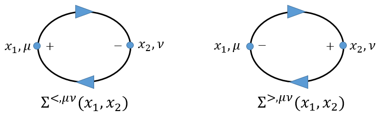
Figure 2: The self-energies Σ<,μν\Sigma^{<,\mu\nu} and Σ>,μν\Sigma^{>,\mu\nu} of vector mesons from quark loops in the quark-meson model. Two quark propagators in the loop may have different flavors corresponding to the vector meson that is not flavor neutral.

We consider the coupling between the vector meson and the quark-antiquark in the quark-meson model (Manohar and Georgi, 1984; Fernandez et al., 1993; Li et al., 1997; Zhao et al., 1998; Zacchi et al., 2015, 2017). Then at lowest order in the coupling constant, the self-energies are from quark loops as shown in Fig. 2

Σ<,μν(x1,x2)\displaystyle\Sigma^{<,\mu\nu}(x_{1},x_{2}) =\displaystyle= Tr[iΓμS<(x1,x2)iΓνS>(x2,x1)],\displaystyle-\text{Tr}\left[i\Gamma^{\mu}S^{<}(x_{1},x_{2})i\Gamma^{\nu}S^{>}(x_{2},x_{1})\right],
Σ>,μν(x1,x2)\displaystyle\Sigma^{>,\mu\nu}(x_{1},x_{2}) =\displaystyle= Tr[iΓμS>(x1,x2)iΓνS<(x2,x1)],\displaystyle-\text{Tr}\left[i\Gamma^{\mu}S^{>}(x_{1},x_{2})i\Gamma^{\nu}S^{<}(x_{2},x_{1})\right], (16)

where S>(x1,x2)S^{>}(x_{1},x_{2}) and S<(x1,x2)S^{<}(x_{1},x_{2}) are two-point Green functions of quarks, iΓμi\Gamma^{\mu} denotes the vertex of the vector meson and quark-antiquark, and the overall minus signs arise from quark loops. Inserting the self-energies (16) into Eq. (14) and taking a Fourier transform with respect to the difference y=x1x2y=x_{1}-x_{2}, we obtain the KB equation for the Wigner function as

{gημ[(p2mV224x2)ipx]\displaystyle\left\{g_{\eta}^{\mu}\left[-\left(p^{2}-m_{V}^{2}-\frac{\hbar^{2}}{4}\partial_{x}^{2}\right)-i\hbar p\cdot\partial_{x}\right]\right. (17)
24xμηx+pμpη+12i(pηxμ+pμηx)}G<,ην(x,p)\displaystyle\left.-\frac{\hbar^{2}}{4}\partial_{x}^{\mu}\partial_{\eta}^{x}+p^{\mu}p_{\eta}+\frac{1}{2}i\hbar\left(p_{\eta}\partial_{x}^{\mu}+p^{\mu}\partial_{\eta}^{x}\right)\right\}G^{<,\eta\nu}(x,p)
=\displaystyle= i2d4p(2π)4{Tr[ΓμS<(x,p+p)ΓαS>(x,p)]G>,αν(x,p)\displaystyle-\frac{i\hbar}{2}\int\frac{d^{4}p^{\prime}}{(2\pi\hbar)^{4}}\left\{\text{Tr}\left[\Gamma^{\mu}S^{<}\left(x,p+p^{\prime}\right)\Gamma_{\alpha}S^{>}\left(x,p^{\prime}\right)\right]G^{>,\alpha\nu}\left(x,p\right)\right.
Tr[ΓμS>(x,p+p)ΓαS<(x,p)]G<,αν(x,p)}\displaystyle\left.-\text{Tr}\left[\Gamma^{\mu}S^{>}\left(x,p+p^{\prime}\right)\Gamma_{\alpha}S^{<}\left(x,p^{\prime}\right)\right]G^{<,\alpha\nu}\left(x,p\right)\right\}
24d4p(2π)4[{Tr[ΓμS<(x,p+p)ΓαS>(x,p)],G>,αν(x,p)}P.B.\displaystyle-\frac{\hbar^{2}}{4}\int\frac{d^{4}p^{\prime}}{(2\pi\hbar)^{4}}\left[\left\{\text{Tr}\left[\Gamma^{\mu}S^{<}\left(x,p+p^{\prime}\right)\Gamma_{\alpha}S^{>}\left(x,p^{\prime}\right)\right],G^{>,\alpha\nu}\left(x,p\right)\right\}_{\text{P.B.}}\right.
{Tr[ΓμS>(x,p+p)ΓαS<(x,p)],G<,αν(x,p)}P.B.],\displaystyle\left.-\left\{\text{Tr}\left[\Gamma^{\mu}S^{>}\left(x,p+p^{\prime}\right)\Gamma_{\alpha}S^{<}\left(x,p^{\prime}\right)\right],G^{<,\alpha\nu}\left(x,p\right)\right\}_{\text{P.B.}}\right],

where the Poisson bracket involves space-time and momentum gradients and is defined as

{A,B}P.B.(xμA)(μpB)(pμA)(μxB).\left\{A,B\right\}_{\text{P.B.}}\equiv(\partial_{x}^{\mu}A)(\partial_{\mu}^{p}B)-(\partial_{p}^{\mu}A)(\partial_{\mu}^{x}B). (18)

In the same way, we obtain from Eq. (15) another KB equation for the Wigner function

{gην[(p2mV224x2)+ipx]\displaystyle\left\{g_{\eta}^{\nu}\left[-\left(p^{2}-m_{V}^{2}-\frac{\hbar^{2}}{4}\partial_{x}^{2}\right)+i\hbar p\cdot\partial_{x}\right]\right. (19)
24xνηx+pνpη12i(pηxν+pνηx)}G<,μη(x,p)\displaystyle\left.-\frac{\hbar^{2}}{4}\partial_{x}^{\nu}\partial_{\eta}^{x}+p^{\nu}p_{\eta}-\frac{1}{2}i\hbar\left(p_{\eta}\partial_{x}^{\nu}+p^{\nu}\partial_{\eta}^{x}\right)\right\}G^{<,\mu\eta}(x,p)
=\displaystyle= i2d4p(2π)4{Gα<,μ(x,p)Tr[ΓαS>(x,p+p)ΓνS<(x,p)]\displaystyle-\frac{i\hbar}{2}\int\frac{d^{4}p^{\prime}}{(2\pi\hbar)^{4}}\left\{G_{\ \ \ \ \alpha}^{<,\mu}(x,p)\text{Tr}\left[\Gamma^{\alpha}S^{>}\left(x,p+p^{\prime}\right)\Gamma^{\nu}S^{<}\left(x,p^{\prime}\right)\right]\right.
Gα>,μ(x,p)Tr[ΓαS<(x,p+p)ΓνS>(x,p)]}\displaystyle\left.-G_{\ \ \ \ \alpha}^{>,\mu}\left(x,p\right)\text{Tr}\left[\Gamma^{\alpha}S^{<}\left(x,p+p^{\prime}\right)\Gamma^{\nu}S^{>}\left(x,p^{\prime}\right)\right]\right\}
24d4p(2π)4[{Gα<,μ(x,p),Tr[ΓαS>(x,p+p)ΓνS<(x,p)]}P.B.\displaystyle-\frac{\hbar^{2}}{4}\int\frac{d^{4}p^{\prime}}{(2\pi\hbar)^{4}}\left[\left\{G_{\ \ \ \ \alpha}^{<,\mu}(x,p),\text{Tr}\left[\Gamma^{\alpha}S^{>}\left(x,p+p^{\prime}\right)\Gamma^{\nu}S^{<}\left(x,p^{\prime}\right)\right]\right\}_{\text{P.B.}}\right.
{Gα>,μ(x,p),Tr[ΓαS<(x,p+p)ΓνS>(x,p)]}P.B.].\displaystyle\left.-\left\{G_{\ \ \ \ \alpha}^{>,\mu}\left(x,p\right),\text{Tr}\left[\Gamma^{\alpha}S^{<}\left(x,p+p^{\prime}\right)\Gamma^{\nu}S^{>}\left(x,p^{\prime}\right)\right]\right\}_{\text{P.B.}}\right].

Taking the difference between Eq. (17) and (19), we are able to derive the Boltzmann equation for the Wigner function at the leading order

pxG<,μν(x,p)14[pμηxG<,ην(x,p)+pνηxG<,μη(x,p)]\displaystyle p\cdot\partial_{x}G^{<,\mu\nu}(x,p)-\frac{1}{4}\left[p^{\mu}\partial_{\eta}^{x}G^{<,\eta\nu}(x,p)+p^{\nu}\partial_{\eta}^{x}G^{<,\mu\eta}(x,p)\right] (20)
=\displaystyle= 14d4p(2π)4{Tr[ΓμS<(x,p+p)ΓαS>(x,p)]G>,αν(x,p)\displaystyle\frac{1}{4}\int\frac{d^{4}p^{\prime}}{(2\pi\hbar)^{4}}\left\{\text{Tr}\left[\Gamma^{\mu}S^{<}\left(x,p+p^{\prime}\right)\Gamma_{\alpha}S^{>}\left(x,p^{\prime}\right)\right]G^{>,\alpha\nu}\left(x,p\right)\right.
Tr[ΓμS>(x,p+p)ΓαS<(x,p)]G<,αν(x,p)}\displaystyle\left.-\text{Tr}\left[\Gamma^{\mu}S^{>}\left(x,p+p^{\prime}\right)\Gamma_{\alpha}S^{<}\left(x,p^{\prime}\right)\right]G^{<,\alpha\nu}\left(x,p\right)\right\}
+14d4p(2π)4{Gα>,μ(x,p)Tr[ΓαS<(x,p+p)ΓνS>(x,p)]\displaystyle+\frac{1}{4}\int\frac{d^{4}p^{\prime}}{(2\pi\hbar)^{4}}\left\{G_{\ \ \ \ \alpha}^{>,\mu}\left(x,p\right)\text{Tr}\left[\Gamma^{\alpha}S^{<}\left(x,p+p^{\prime}\right)\Gamma^{\nu}S^{>}\left(x,p^{\prime}\right)\right]\right.
Gα<,μ(x,p)Tr[ΓαS>(x,p+p)ΓνS<(x,p)]},\displaystyle\left.-G_{\ \ \ \ \alpha}^{<,\mu}(x,p)\text{Tr}\left[\Gamma^{\alpha}S^{>}\left(x,p+p^{\prime}\right)\Gamma^{\nu}S^{<}\left(x,p^{\prime}\right)\right]\right\},

where we have neglected terms with Poisson brackets and those proportional to pηp_{\eta} in the left-hand-side since their contraction with the leading-order G<,ην(x,p)G^{<,\eta\nu}(x,p) and G<,μη(x,p)G^{<,\mu\eta}(x,p) is vanishing. In the next section we will rewrite the above Boltzmann equation in terms of MVSDs for vector mesons, quarks and antiquarks.

IV Spin density matrix for quark coalescence and dissociation

The two-point Green functions S>(x,p)S^{>}\left(x,p\right) and S<(x,p)S^{<}\left(x,p\right) for quarks are given by (Sheng et al., 2021)

S<(x,p)\displaystyle S^{<}(x,p) =\displaystyle= (2π)θ(p0)δ(p2mq2)r,su(r,𝐩)u¯(s,𝐩)frs(+)(x,𝐩)\displaystyle-(2\pi\hbar)\theta(p_{0})\delta(p^{2}-m_{q}^{2})\sum_{r,s}u(r,\mathbf{p})\overline{u}(s,\mathbf{p})f_{rs}^{(+)}(x,\mathbf{p})
(2π)θ(p0)δ(p2mq2)r,sv(s,𝐩)v¯(r,𝐩)[δrsfrs()(x,𝐩)],\displaystyle-(2\pi\hbar)\theta(-p_{0})\delta(p^{2}-m_{q}^{2})\sum_{r,s}v(s,-\mathbf{p})\overline{v}(r,-\mathbf{p})\left[\delta_{rs}-f_{rs}^{(-)}(x,-\mathbf{p})\right],
S>(x,p)\displaystyle S^{>}(x,p) =\displaystyle= (2π)θ(p0)δ(p2mq2)r,su(r,𝐩)u¯(s,𝐩)[δrsfrs(+)(x,𝐩)]\displaystyle(2\pi\hbar)\theta(p_{0})\delta(p^{2}-m_{q}^{2})\sum_{r,s}u(r,\mathbf{p})\overline{u}(s,\mathbf{p})\left[\delta_{rs}-f_{rs}^{(+)}(x,\mathbf{p})\right] (21)
+(2π)θ(p0)δ(p2mq2)r,sv(s,𝐩)v¯(r,𝐩)frs()(x,𝐩),\displaystyle+(2\pi\hbar)\theta(-p_{0})\delta(p^{2}-m_{q}^{2})\sum_{r,s}v(s,-\mathbf{p})\overline{v}(r,-\mathbf{p})f_{rs}^{(-)}(x,-\mathbf{p}),

where frs(+)f_{rs}^{(+)} and frs()f_{rs}^{(-)} are MVSD for quarks and antiquarks respectively. We can parameterize them as

frs(+)(x,𝐩)\displaystyle f_{rs}^{(+)}(x,\mathbf{p}) =\displaystyle= 12fq(x,𝐩)[δrsPμq(x,𝐩)nj(+)μ(𝐩)τrsj],\displaystyle\frac{1}{2}f_{q}(x,\mathbf{p})\left[\delta_{rs}-P_{\mu}^{q}(x,\mathbf{p})n_{j}^{(+)\mu}(\mathbf{p})\tau_{rs}^{j}\right],
frs()(x,𝐩)\displaystyle f_{rs}^{(-)}(x,-\mathbf{p}) =\displaystyle= 12fq¯(x,𝐩)[δrsPμq¯(x,𝐩)nj()μ(𝐩)τrsj],\displaystyle\frac{1}{2}f_{\overline{q}}(x,-\mathbf{p})\left[\delta_{rs}-P_{\mu}^{\overline{q}}(x,-\mathbf{p})n_{j}^{(-)\mu}(\mathbf{p})\tau_{rs}^{j}\right], (22)

where fq(x,𝐩)f_{q}(x,\mathbf{p}) and fq¯(x,𝐩)f_{\overline{q}}(x,-\mathbf{p}) are MVSDs for quarks and antiquarks respectively, and Pqμ(x,𝐩)P_{q}^{\mu}(x,\mathbf{p}) and Pq¯μ(x,𝐩)P_{\overline{q}}^{\mu}(x,-\mathbf{p}) are polarization four-vectors for quarks and antiquarks respectively. The spin direction four-vectors for quarks and antiquarks are given by

nj(+)μ(𝐩)\displaystyle n_{j}^{(+)\mu}(\mathbf{p}) \displaystyle\equiv nμ(𝐧j,𝐩,mq)=(𝐧j𝐩mq,𝐧j+(𝐧j𝐩)𝐩mq(E𝐩q+mq)),\displaystyle n^{\mu}(\mathbf{n}_{j},\mathbf{p},m_{q})=\left(\frac{\mathbf{n}_{j}\cdot{\bf p}}{m_{q}},\mathbf{n}_{j}+\frac{(\mathbf{n}_{j}\cdot{\bf p}){\bf p}}{m_{q}(E_{{\bf p}}^{q}+m_{q})}\right),
nj()μ(𝐩)\displaystyle n_{j}^{(-)\mu}(\mathbf{p}) \displaystyle\equiv nμ(𝐧j,𝐩,mq¯)=(𝐧j𝐩mq¯,𝐧j+(𝐧j𝐩)𝐩mq¯(E𝐩q¯+mq¯)),\displaystyle n^{\mu}(\mathbf{n}_{j},-\mathbf{p},m_{\overline{q}})=\left(-\frac{\mathbf{n}_{j}\cdot{\bf p}}{m_{\overline{q}}},\mathbf{n}_{j}+\frac{(\mathbf{n}_{j}\cdot{\bf p}){\bf p}}{m_{\overline{q}}(E_{{\bf p}}^{\overline{q}}+m_{\overline{q}})}\right), (23)

where 𝐧j\mathbf{n}_{j} for j=1,2,3j=1,2,3 are three basis unit vectors that form a Cartesian coordinate system in the particle’s rest frame with 𝐧3\mathbf{n}_{3} being the spin quantization direction, and nj(+)μn_{j}^{(+)\mu} and nj()μn_{j}^{(-)\mu} are the Lorentz transformed four-vectors of 𝐧j\mathbf{n}_{j} for quarks and antiquarks respectively which obey the sum rules

nj(+)μ(𝐩)nj(+)ν(𝐩)\displaystyle n_{j}^{(+)\mu}(\mathbf{p})n_{j}^{(+)\nu}(\mathbf{p}) =\displaystyle= (gμνpμpνmq2),\displaystyle-\left(g^{\mu\nu}-\frac{p^{\mu}p^{\nu}}{m_{q}^{2}}\right),
nj()μ(𝐩)nj()ν(𝐩)\displaystyle n_{j}^{(-)\mu}(\mathbf{p})n_{j}^{(-)\nu}(\mathbf{p}) =\displaystyle= (gμνp¯μp¯νmq¯2),\displaystyle-\left(g^{\mu\nu}-\frac{\overline{p}^{\mu}\overline{p}^{\nu}}{m_{\overline{q}}^{2}}\right), (24)

where pμ=(Epq,𝐩)p^{\mu}=(E_{p}^{q},\mathbf{p}) and p¯μ=(Epq¯,𝐩)\overline{p}^{\mu}=(E_{p}^{\overline{q}},-\mathbf{p}). We note that frs(+)(x,𝐩)f_{rs}^{(+)}(x,\mathbf{p}) and frs()(x,𝐩)f_{rs}^{(-)}(x,-\mathbf{p}) are actually the transpose of those MVSDs defined in Eqs. (117)-(118) of Ref. (Sheng et al., 2021) in spin indices. We can flip the sign of the three-momentum, 𝐩𝐩\mathbf{p}\rightarrow-\mathbf{p}, in frs()(x,𝐩)f_{rs}^{(-)}(x,-\mathbf{p}) to obtain

frs()(x,𝐩)=12fq¯(x,𝐩)[δrsPμq¯(x,𝐩)nj()μ(𝐩)τrsj],f_{rs}^{(-)}(x,\mathbf{p})=\frac{1}{2}f_{\overline{q}}(x,\mathbf{p})\left[\delta_{rs}-P_{\mu}^{\overline{q}}(x,\mathbf{p})n_{j}^{(-)\mu}(-\mathbf{p})\tau_{rs}^{j}\right], (25)

where nj()μ(𝐩)n_{j}^{(-)\mu}(-\mathbf{p}) has the same form as nj(+)μ(𝐩)n_{j}^{(+)\mu}(\mathbf{p}) except the quark mass. Note that in the self-energy (16) of the vector meson that is not flavor neutral, S<(x,p)S^{<}(x,p) and S>(x,p)S^{>}(x,p) may involve different flavors of quarks and antiquarks.

Inserting S<(x,p)S^{<}(x,p), S>(x,p)S^{>}(x,p), G<,μν(x,p)G^{<,\mu\nu}(x,p), and G>,μν(x,p)G^{>,\mu\nu}(x,p) in Eqs. (21), (11) and (13) into Eq. (20), the Boltzmann equation can be put into the following form

pxG<,μν(x,p)14[pμηxG<,ην(x,p)+pνηxG<,μη(x,p)]\displaystyle p\cdot\partial_{x}G^{<,\mu\nu}(x,p)-\frac{1}{4}\left[p^{\mu}\partial_{\eta}^{x}G^{<,\eta\nu}(x,p)+p^{\nu}\partial_{\eta}^{x}G^{<,\mu\eta}(x,p)\right] (26)
=\displaystyle= 14(2π)d4pδ(p2mq¯2)δ[(p+p)2mq2]δ(p2mV2)\displaystyle\frac{1}{4(2\pi\hbar)}\int d^{4}p^{\prime}\delta(p^{\prime 2}-m_{\overline{q}}^{2})\delta\left[(p+p^{\prime})^{2}-m_{q}^{2}\right]\delta(p^{2}-m_{V}^{2})
×{θ(p0)θ(p0+p0)θ(p0)I+++\displaystyle\times\left\{\theta(p_{0}^{\prime})\theta\left(p_{0}+p_{0}^{\prime}\right)\theta(p_{0})I_{+++}\right.
+θ(p0)θ(p0+p0)θ(p0)I++\displaystyle+\theta(p_{0}^{\prime})\theta\left(p_{0}+p_{0}^{\prime}\right)\theta(-p_{0})I_{++-}
+θ(p0)θ(p0p0)θ(p0)I+\displaystyle+\theta(p_{0}^{\prime})\theta\left(-p_{0}-p_{0}^{\prime}\right)\theta(-p_{0})I_{+--}
+θ(p0)θ(p0+p0)θ(p0)I++\displaystyle+\theta(-p_{0}^{\prime})\theta\left(p_{0}+p_{0}^{\prime}\right)\theta(p_{0})I_{-++}
+θ(p0)θ(p0p0)θ(p0)I+\displaystyle+\theta(-p_{0}^{\prime})\theta\left(-p_{0}-p_{0}^{\prime}\right)\theta(p_{0})I_{--+}
+θ(p0)θ(p0p0)θ(p0)I}.\displaystyle\left.+\theta(-p_{0}^{\prime})\theta\left(-p_{0}-p_{0}^{\prime}\right)\theta(-p_{0})I_{---}\right\}.

The terms IijkI_{ijk}, with i,j,k=±i,j,k=\pm representing the positive/negative energy, correspond to all possible processes at lowest order in the coupling constant, as shown in Table 1. In Eq. (26), I+I_{-+-} and I++I_{+-+} are absent due to incompatibility of theta functions, and I++I_{-++} and I+I_{+--} contain the coalescence of quark-antiquark to the vector meson and vice versa, but I++I_{-++} corresponds to the positive energy sector of the two-point function for the vector meson while I+I_{+--} corresponds to the negative energy sector. All terms except I++I_{-++} and I+I_{+--} are vanishing for on-shell quarks, antiquarks and mesons at the one-loop level of the selfenergy. We distinguish mqm_{q} from mq¯m_{\overline{q}} in Eq. (26) since the quark and antiquark may have different flavors for the vector meson that is not flavor neutral so the meson and its antiparticle are not the same particle.

I+++I_{+++} I++I_{++-} I+I_{+--} I++I_{-++} I+I_{--+} II_{---}
qq+Mq\rightarrow q+M q+M¯qq+\overline{M}\rightarrow q M¯q+q¯\overline{M}\rightarrow q+\overline{q} q+q¯Mq+\overline{q}\rightarrow M q¯q¯+M\overline{q}\rightarrow\overline{q}+M q¯+M¯q¯\overline{q}+\overline{M}\rightarrow\overline{q}
q+Mqq+M\rightarrow q qq+M¯q\rightarrow q+\overline{M} q+q¯M¯q+\overline{q}\rightarrow\overline{M} Mq+q¯M\rightarrow q+\overline{q} q¯+Mq¯\overline{q}+M\rightarrow\overline{q} q¯q¯+M¯\overline{q}\rightarrow\overline{q}+\overline{M}
Table 1: Collision terms in the Boltzmann equation. All terms except I++I_{-++} and I+I_{+--} are vanishing for on-shell quarks, antiquarks and mesons at the one-loop level of the selfenergy.

In this paper, we are interested in the contribution from the coalescence and dissociation processes corresponding to I++I_{-++}. The coalescence is regarded as one of the main processes for particle production in heavy-ion collisions (Greco et al., 2003a; Fries et al., 2003a; Greco et al., 2003b; Fries et al., 2003b; Greco et al., 2004; Zhao et al., 2020). So the spin Boltzmann equation for the vector meson’s MVSD reads

pxfλ1λ2(x,𝐩)\displaystyle p\cdot\partial_{x}f_{\lambda_{1}\lambda_{2}}(x,\mathbf{p}) (27)
=\displaystyle= 116r1,s1,r2,s2,λ1,λ2d3𝐩(2π)31Epq¯E𝐩𝐩q2πδ(EpVEpq¯E𝐩𝐩q)\displaystyle\frac{1}{16}\sum_{r_{1},s_{1},r_{2},s_{2},\lambda_{1}^{\prime},\lambda_{2}^{\prime}}\int\frac{d^{3}\mathbf{p}^{\prime}}{(2\pi\hbar)^{3}}\frac{1}{E_{p^{\prime}}^{\overline{q}}E_{{\bf p}-{\bf p}^{\prime}}^{q}}2\pi\hbar\delta\left(E_{p}^{V}-E_{p^{\prime}}^{\overline{q}}-E_{{\bf p}-{\bf p}^{\prime}}^{q}\right)
×{δλ2λ2ϵμ(λ1,𝐩)ϵα(λ1,𝐩)Tr[Γαv(s1,𝐩)v¯(r1,𝐩)Γμu(r2,𝐩𝐩)u¯(s2,𝐩𝐩)]\displaystyle\times\left\{\delta_{\lambda_{2}\lambda_{2}^{\prime}}\epsilon_{\mu}^{\ast}(\lambda_{1},{\bf p})\epsilon^{\alpha}\left(\lambda_{1}^{\prime},{\bf p}\right)\text{Tr}\left[\Gamma_{\alpha}v(s_{1},{\bf p}^{\prime})\overline{v}(r_{1},{\bf p}^{\prime})\Gamma^{\mu}u(r_{2},\mathbf{p}-{\bf p}^{\prime})\overline{u}(s_{2},\mathbf{p}-{\bf p}^{\prime})\right]\right.
+δλ1λ1ϵν(λ2,𝐩)ϵα(λ2,𝐩)Tr[Γνv(s1,𝐩)v¯(r1,𝐩)Γαu(r2,𝐩𝐩)u¯(s2,𝐩𝐩)]}\displaystyle+\left.\delta_{\lambda_{1}\lambda_{1}^{\prime}}\epsilon_{\nu}(\lambda_{2},{\bf p})\epsilon_{\alpha}^{\ast}\left(\lambda_{2}^{\prime},{\bf p}\right)\text{Tr}\left[\Gamma^{\nu}v(s_{1},{\bf p}^{\prime})\overline{v}(r_{1},{\bf p}^{\prime})\Gamma^{\alpha}u(r_{2},\mathbf{p}-{\bf p}^{\prime})\overline{u}(s_{2},\mathbf{p}-{\bf p}^{\prime})\right]\right\}
×{fr1s1()(x,𝐩)fr2s2(+)(x,𝐩𝐩)[δλ1λ2+fλ1λ2(x,𝐩)]\displaystyle\times\left\{f_{r_{1}s_{1}}^{(-)}(x,{\bf p}^{\prime})f_{r_{2}s_{2}}^{(+)}(x,\mathbf{p}-\mathbf{p}^{\prime})\left[\delta_{\lambda_{1}^{\prime}\lambda_{2}^{\prime}}+f_{\lambda_{1}^{\prime}\lambda_{2}^{\prime}}(x,\mathbf{p})\right]\right.
[δr1s1fr1s1()(x,𝐩)][δr2s2fr2s2(+)(x,𝐩𝐩)]fλ1λ2(x,𝐩)},\displaystyle\left.-\left[\delta_{r_{1}s_{1}}-f_{r_{1}s_{1}}^{(-)}(x,{\bf p}^{\prime})\right]\left[\delta_{r_{2}s_{2}}-f_{r_{2}s_{2}}^{(+)}(x,\mathbf{p}-\mathbf{p}^{\prime})\right]f_{\lambda_{1}^{\prime}\lambda_{2}^{\prime}}(x,\mathbf{p})\right\},

where λ1\lambda_{1}, λ2\lambda_{2}, λ1\lambda_{1}^{\prime} and λ2\lambda_{2}^{\prime} denote the spin states along the spin quantization direction, and Γα\Gamma^{\alpha} is the qq¯Vq\overline{q}V vertex given by

ΓαgVB(𝐩𝐩,𝐩)γα,\Gamma^{\alpha}\approx g_{V}B(\mathbf{p}-\mathbf{p}^{\prime},\mathbf{p}^{\prime})\gamma^{\alpha}, (28)

where gVg_{V} is the coupling constant of the vector meson and quark-antiquark, and B(𝐩𝐩,𝐩)B(\mathbf{p}-\mathbf{p}^{\prime},\mathbf{p}^{\prime}) denotes the Bethe-Salpeter wave function of the ϕ\phi meson (Xu et al., 2019, 2021) in the following parametrization form

B(𝐩𝐩,𝐩)=1exp{[(E𝐩𝐩sE𝐩s¯)2(𝐩2𝐩)2]/σ2}[(E𝐩𝐩sE𝐩s¯)2(𝐩2𝐩)2]/σ2,B(\mathbf{p}-\mathbf{p}^{\prime},\mathbf{p}^{\prime})=\frac{1-\exp\left\{-\left[(E_{\mathbf{p}-\mathbf{p}^{\prime}}^{s}-E_{\mathbf{p}^{\prime}}^{\overline{s}})^{2}-(\mathbf{p}-2\mathbf{p}^{\prime})^{2}\right]/\sigma^{2}\right\}}{\left[(E_{\mathbf{p}-\mathbf{p}^{\prime}}^{s}-E_{\mathbf{p}^{\prime}}^{\overline{s}})^{2}-(\mathbf{p}-2\mathbf{p}^{\prime})^{2}\right]/\sigma^{2}}, (29)

with σ0.522\sigma\approx 0.522 GeV being the width parameter of the wave function. The derivation of Eq. (27) is given in Appendix A. We see that there is a gain term and a loss term in Eq. (27). In heavy ion collisions, the distribution functions are normally much less than 1, fλ1λ2(x,𝐩)frs(+)frs()1f_{\lambda_{1}\lambda_{2}}(x,\mathbf{p})\sim f_{rs}^{(+)}\sim f_{rs}^{(-)}\ll 1, so Eq. (27) can be approximated as

pEpVxfλ1λ2(x,𝐩)Rλ1λ2coal(𝐩)Rdiss(𝐩)fλ1λ2(x,𝐩),\frac{p}{E_{p}^{V}}\cdot\partial_{x}f_{\lambda_{1}\lambda_{2}}(x,\mathbf{p})\approx R_{\lambda_{1}\lambda_{2}}^{\mathrm{coal}}(\mathbf{p})-R^{\mathrm{diss}}(\mathbf{p})f_{\lambda_{1}\lambda_{2}}(x,\mathbf{p}), (30)

where Rλ1λ2coalR_{\lambda_{1}\lambda_{2}}^{\mathrm{coal}} and Rλ1λ2dissR_{\lambda_{1}\lambda_{2}}^{\mathrm{diss}} denote the coalescence and dissociation rates for the vector meson, i.e. the rates of q+q¯Mq+\overline{q}\rightarrow M and Mq+q¯M\rightarrow q+\overline{q} respectively, defined as

Rλ1λ2coal(𝐩)\displaystyle R_{\lambda_{1}\lambda_{2}}^{\mathrm{coal}}(\mathbf{p}) =\displaystyle= 18(2π)2r1,s1,r2,s2d3𝐩1Epq¯E𝐩𝐩qEpV\displaystyle\frac{1}{8(2\pi\hbar)^{2}}\sum_{r_{1},s_{1},r_{2},s_{2}}\int d^{3}\mathbf{p}^{\prime}\frac{1}{E_{p^{\prime}}^{\overline{q}}E_{{\bf p}-{\bf p}^{\prime}}^{q}E_{p}^{V}} (31)
×δ(EpVEpq¯E𝐩𝐩q)ϵα(λ1,𝐩)ϵβ(λ2,𝐩)\displaystyle\times\delta\left(E_{p}^{V}-E_{p^{\prime}}^{\overline{q}}-E_{{\bf p}-{\bf p}^{\prime}}^{q}\right)\epsilon_{\alpha}^{\ast}(\lambda_{1},{\bf p})\epsilon_{\beta}(\lambda_{2},{\bf p})
×Tr[Γβv(s1,𝐩)v¯(r1,𝐩)Γαu(r2,𝐩𝐩)u¯(s2,𝐩𝐩)]\displaystyle\times\text{Tr}\left[\Gamma^{\beta}v(s_{1},{\bf p}^{\prime})\overline{v}(r_{1},{\bf p}^{\prime})\Gamma^{\alpha}u(r_{2},\mathbf{p}-{\bf p}^{\prime})\overline{u}(s_{2},\mathbf{p}-{\bf p}^{\prime})\right]
×fr1s1()(x,𝐩)fr2s2(+)(x,𝐩𝐩),\displaystyle\times f_{r_{1}s_{1}}^{(-)}(x,{\bf p}^{\prime})f_{r_{2}s_{2}}^{(+)}(x,\mathbf{p}-{\bf p}^{\prime}),
Rdiss(𝐩)\displaystyle R^{\mathrm{diss}}(\mathbf{p}) =\displaystyle= 112(2π)2r1,r2d3𝐩1Epq¯E𝐩𝐩qEpV\displaystyle-\frac{1}{12(2\pi\hbar)^{2}}\sum_{r_{1},r_{2}}\int d^{3}\mathbf{p}^{\prime}\frac{1}{E_{p^{\prime}}^{\overline{q}}E_{{\bf p}-{\bf p}^{\prime}}^{q}E_{p}^{V}} (32)
×δ(EpVEpq¯E𝐩𝐩q)(gαβpαpβmV2)\displaystyle\times\delta\left(E_{p}^{V}-E_{p^{\prime}}^{\overline{q}}-E_{{\bf p}-{\bf p}^{\prime}}^{q}\right)\left(g_{\alpha\beta}-\frac{p_{\alpha}p_{\beta}}{m_{V}^{2}}\right)
×Tr{Γβ(pγmq¯)Γα[(pp)γ+mq]}.\displaystyle\times\text{Tr}\left\{\Gamma^{\beta}\left(p^{\prime}\cdot\gamma-m_{\overline{q}}\right)\Gamma^{\alpha}\left[(p-p^{\prime})\cdot\gamma+m_{q}\right]\right\}.

Note that Rdiss(𝐩)R^{\mathrm{diss}}(\mathbf{p}) does not depend on the MVSDs of the quark, antiquark and the vector meson, therefore it is independent of the quark polarization. Schematically the formal solution to Eq. (30) reads

fλ1λ2(x,𝐩)\displaystyle f_{\lambda_{1}\lambda_{2}}(x,\mathbf{p}) \displaystyle\sim Rλ1λ2coal(𝐩)Rdiss(𝐩)[1exp(Rdiss(𝐩)Δt)]\displaystyle\frac{R_{\lambda_{1}\lambda_{2}}^{\mathrm{coal}}(\mathbf{p})}{R^{\mathrm{diss}}(\mathbf{p})}\left[1-\exp\left(-R^{\mathrm{diss}}(\mathbf{p})\Delta t\right)\right] (33)
\displaystyle\sim {Rλ1λ2coal(𝐩)Δt,forΔt1/Rdiss(𝐩)Rλ1λ2coal(𝐩)Rdiss(𝐩),forΔt1/Rdiss(𝐩)\displaystyle\begin{cases}R_{\lambda_{1}\lambda_{2}}^{\mathrm{coal}}(\mathbf{p})\Delta t,&\mathrm{for}\;\Delta t\ll 1/R^{\mathrm{diss}}(\mathbf{p})\\ \frac{R_{\lambda_{1}\lambda_{2}}^{\mathrm{coal}}(\mathbf{p})}{R^{\mathrm{diss}}(\mathbf{p})},&\mathrm{for}\;\Delta t\gg 1/R^{\mathrm{diss}}(\mathbf{p})\end{cases}

if fλ1λ2(x,𝐩)f_{\lambda_{1}\lambda_{2}}(x,\mathbf{p}) for the vector meson at the initial time is assumed to be zero, where Δt\Delta t is the formation time of the vector meson.

The spin density matrix element ρλ1λ2V\rho_{\lambda_{1}\lambda_{2}}^{V} is assumed to be proportional to fλ1λ2(x,𝐩)f_{\lambda_{1}\lambda_{2}}(x,\mathbf{p}) which is Rλ1λ2coal(𝐩)ΔtR_{\lambda_{1}\lambda_{2}}^{\mathrm{coal}}(\mathbf{p})\Delta t if Δt1/Rdiss(𝐩)\Delta t\ll 1/R^{\mathrm{diss}}(\mathbf{p}) or Rλ1λ2coal(𝐩)/Rdiss(𝐩)R_{\lambda_{1}\lambda_{2}}^{\mathrm{coal}}(\mathbf{p})/R^{\mathrm{diss}}(\mathbf{p}) if Δt1/Rdiss(𝐩)\Delta t\gg 1/R^{\mathrm{diss}}(\mathbf{p}). In both cases, ρλ1λ2V\rho_{\lambda_{1}\lambda_{2}}^{V} is proportional to Rλ1λ2coal(𝐩)R_{\lambda_{1}\lambda_{2}}^{\mathrm{coal}}(\mathbf{p}) times a constant independent of the spin states of the vector meson. Here we assume that the coalescence of the vector meson takes place in a relatively short time, so we have

ρλ1λ2V(x,𝐩)\displaystyle\rho_{\lambda_{1}\lambda_{2}}^{V}(x,{\bf p}) \displaystyle\approx Δt8r1,s1,r2,s2d3𝐩(2π)31Epq¯E𝐩𝐩qEpV\displaystyle\frac{\Delta t}{8}\sum_{r_{1},s_{1},r_{2},s_{2}}\int\frac{d^{3}\mathbf{p}^{\prime}}{(2\pi\hbar)^{3}}\frac{1}{E_{p^{\prime}}^{\overline{q}}E_{{\bf p}-{\bf p}^{\prime}}^{q}E_{p}^{V}} (34)
×2πδ(EpVEpq¯E𝐩𝐩q)ϵα(λ1,𝐩)ϵβ(λ2,𝐩)\displaystyle\times 2\pi\hbar\delta\left(E_{p}^{V}-E_{p^{\prime}}^{\overline{q}}-E_{{\bf p}-{\bf p}^{\prime}}^{q}\right)\epsilon_{\alpha}^{\ast}(\lambda_{1},{\bf p})\epsilon_{\beta}(\lambda_{2},{\bf p})
×Tr[Γβv(s1,𝐩)v¯(r1,𝐩)Γαu(r2,𝐩𝐩)u¯(s2,𝐩𝐩)]\displaystyle\times\text{Tr}\left[\Gamma^{\beta}v(s_{1},{\bf p}^{\prime})\overline{v}(r_{1},{\bf p}^{\prime})\Gamma^{\alpha}u(r_{2},\mathbf{p}-{\bf p}^{\prime})\overline{u}(s_{2},\mathbf{p}-{\bf p}^{\prime})\right]
×fr1s1(q¯)(x,𝐩)fr2s2(q)(x,𝐩𝐩),\displaystyle\times f_{r_{1}s_{1}}^{(\overline{q})}(x,{\bf p}^{\prime})f_{r_{2}s_{2}}^{(q)}(x,\mathbf{p}-{\bf p}^{\prime}),

where we have changed the notation to frs(q/q¯)f_{rs}^{(q/\overline{q})} from frs(±)f_{rs}^{(\pm)}. The spin density matrix element (34) can be put into a compact form with an explicit dependence on the polarization vector of the quark and antiquark

ρλ1λ2V(x,𝐩)\displaystyle\rho_{\lambda_{1}\lambda_{2}}^{V}(x,{\bf p}) =\displaystyle= Δt32d3𝐩(2π)31Epq¯E𝐩𝐩qEpVfq¯(x,𝐩)fq(x,𝐩𝐩)\displaystyle\frac{\Delta t}{32}\int\frac{d^{3}\mathbf{p}^{\prime}}{(2\pi\hbar)^{3}}\frac{1}{E_{p^{\prime}}^{\overline{q}}E_{{\bf p}-{\bf p}^{\prime}}^{q}E_{p}^{V}}f_{\overline{q}}(x,\mathbf{p}^{\prime})f_{q}(x,\mathbf{p}-\mathbf{p}^{\prime}) (35)
×2πδ(EpVEpq¯E𝐩𝐩q)ϵα(λ1,𝐩)ϵβ(λ2,𝐩)\displaystyle\times 2\pi\hbar\delta\left(E_{p}^{V}-E_{p^{\prime}}^{\overline{q}}-E_{{\bf p}-{\bf p}^{\prime}}^{q}\right)\epsilon_{\alpha}^{\ast}(\lambda_{1},{\bf p})\epsilon_{\beta}(\lambda_{2},{\bf p})
×Tr{Γβ(pγmq¯)[1+γ5γPq¯(x,𝐩)]Γα\displaystyle\times\text{Tr}\left\{\Gamma^{\beta}\left(p^{\prime}\cdot\gamma-m_{\overline{q}}\right)\left[1+\gamma_{5}\gamma\cdot P^{\overline{q}}(x,\mathbf{p}^{\prime})\right]\Gamma^{\alpha}\right.
×[(pp)γ+mq][1+γ5γPq(x,𝐩𝐩)]},\displaystyle\times\left.\left[(p-p^{\prime})\cdot\gamma+m_{q}\right]\left[1+\gamma_{5}\gamma\cdot P^{q}(x,\mathbf{p}-\mathbf{p}^{\prime})\right]\right\},

where pμ=(Epq,𝐩)p^{\mu}=(E_{p}^{q},\mathbf{p}) and pμ=(Epq¯,𝐩)p^{\prime\mu}=(E_{p^{\prime}}^{\overline{q}},\mathbf{p}^{\prime}). The derivation of the expression inside the trace is given in Appendix B. The contraction of ϵα(λ1,𝐩)\epsilon_{\alpha}^{\ast}(\lambda_{1},{\bf p}) and ϵβ(λ2,𝐩)\epsilon_{\beta}(\lambda_{2},{\bf p}) with the trace can be worked out and the result is given by Eq. (86). The normalized ρλ1λ2V(x,𝐩)\rho_{\lambda_{1}\lambda_{2}}^{V}(x,{\bf p}) is defined as

ρ¯λ1λ2V(x,𝐩)=ρλ1λ2V(x,𝐩)Tr(ρV),\overline{\rho}_{\lambda_{1}\lambda_{2}}^{V}(x,{\bf p})=\frac{\rho_{\lambda_{1}\lambda_{2}}^{V}(x,{\bf p})}{\mathrm{Tr}(\rho_{V})}, (36)

where Tr(ρV)\mathrm{Tr}(\rho_{V}) is the trace of the spin density matrix and is evaluated using Eq. (87) and ρλ1λ2V(x,𝐩)\rho_{\lambda_{1}\lambda_{2}}^{V}(x,{\bf p}) is evaluated using Eq. (86).

For quarkonium vector mesons such as ϕ\phi mesons with mq=mq¯m_{q}=m_{\overline{q}}, ρλ1λ2V(x,𝐩)\rho_{\lambda_{1}\lambda_{2}}^{V}(x,{\bf p}) and Tr(ρV)\mathrm{Tr}(\rho_{V}) can be simplified as

ρλ1λ2V(x,𝐩)\displaystyle\rho_{\lambda_{1}\lambda_{2}}^{V}(x,{\bf p}) =\displaystyle= Δt8gV2d3𝐩(2π)31Epq¯E𝐩𝐩qEpVfq¯(x,𝐩)fq(x,𝐩𝐩)\displaystyle-\frac{\Delta t}{8}g_{V}^{2}\int\frac{d^{3}\mathbf{p}^{\prime}}{(2\pi\hbar)^{3}}\frac{1}{E_{p^{\prime}}^{\overline{q}}E_{{\bf p}-{\bf p}^{\prime}}^{q}E_{p}^{V}}f_{\overline{q}}(x,\mathbf{p}^{\prime})f_{q}(x,\mathbf{p}-\mathbf{p}^{\prime}) (37)
×2πδ(EpVEpq¯E𝐩𝐩q)B2(𝐩𝐩,𝐩)ϵα(λ1,𝐩)ϵβ(λ2,𝐩)\displaystyle\times 2\pi\hbar\delta\left(E_{p}^{V}-E_{p^{\prime}}^{\overline{q}}-E_{{\bf p}-{\bf p}^{\prime}}^{q}\right)B^{2}(\mathbf{p}-\mathbf{p}^{\prime},\mathbf{p}^{\prime})\epsilon_{\alpha}^{\ast}(\lambda_{1},{\bf p})\epsilon_{\beta}(\lambda_{2},{\bf p})
×{(pαPq¯β+pβPq¯α)(pPq)(pαPqβ+pβPqα)(pPq¯)\displaystyle\times\left\{\left(p^{\prime\alpha}P_{\overline{q}}^{\beta}+p^{\prime\beta}P_{\overline{q}}^{\alpha}\right)(p^{\prime}\cdot P_{q})-\left(p^{\prime\alpha}P_{q}^{\beta}+p^{\prime\beta}P_{q}^{\alpha}\right)(p\cdot P_{\overline{q}})\right.
+2pαpβ(1Pq¯Pq)+gαβ[pp+(pPq)(pPq¯)]\displaystyle+2p^{\prime\alpha}p^{\prime\beta}(1-P_{\overline{q}}\cdot P_{q})+g^{\alpha\beta}\left[p^{\prime}\cdot p+(p^{\prime}\cdot P_{q})(p\cdot P_{\overline{q}})\right]
+(pp)(Pq¯αPqβ+PqαPq¯βgαβPq¯Pq)\displaystyle+(p\cdot p^{\prime})\left(P_{\overline{q}}^{\alpha}P_{q}^{\beta}+P_{q}^{\alpha}P_{\overline{q}}^{\beta}-g^{\alpha\beta}P_{\overline{q}}\cdot P_{q}\right)
imqεαβμνpμ(Pνq+Pνq¯)},\displaystyle\left.-im_{q}\varepsilon^{\alpha\beta\mu\nu}p_{\mu}(P_{\nu}^{q}+P_{\nu}^{\overline{q}})\right\},
Tr(ρV)\displaystyle\mathrm{Tr}(\rho_{V}) =\displaystyle= Δt8gV2d3𝐩(2π)31Epq¯E𝐩𝐩qEpVfq¯(x,𝐩)fq(x,𝐩𝐩)\displaystyle\frac{\Delta t}{8}g_{V}^{2}\int\frac{d^{3}\mathbf{p}^{\prime}}{(2\pi\hbar)^{3}}\frac{1}{E_{p^{\prime}}^{\overline{q}}E_{{\bf p}-{\bf p}^{\prime}}^{q}E_{p}^{V}}f_{\overline{q}}(x,\mathbf{p}^{\prime})f_{q}(x,\mathbf{p}-\mathbf{p}^{\prime}) (38)
×2πδ(EpVEpq¯E𝐩𝐩q)B2(𝐩𝐩,𝐩)\displaystyle\times 2\pi\hbar\delta\left(E_{p}^{V}-E_{p^{\prime}}^{\overline{q}}-E_{{\bf p}-{\bf p}^{\prime}}^{q}\right)B^{2}(\mathbf{p}-\mathbf{p}^{\prime},\mathbf{p}^{\prime})
×[2mq2(Pq¯Pq)+mV2+2mq2],\displaystyle\times\left[-2m_{q}^{2}(P_{\overline{q}}\cdot P_{q})+m_{V}^{2}+2m_{q}^{2}\right],

where we have used the short-hand notation PqPq(x,𝐩𝐩)P_{q}\equiv P_{q}(x,\mathbf{p}-\mathbf{p}^{\prime}) and Pq¯Pq¯(x,𝐩)P_{\overline{q}}\equiv P_{\overline{q}}(x,\mathbf{p}^{\prime}). Equations (37) and (38) will be used in the next section for evaluating spin density matrix elements for ϕ\phi mesons.

V Spin density matrix elements for ϕ\phi mesons

Now we consider the vector meson made of a quark and its antiquark, the so-called quarkonium. For the quarkonium vector meson such as the ϕ\phi meson, the polarization distributions in phase space in Eq. (35) are given by (Becattini et al., 2013, 2017; Fang et al., 2016; Yang et al., 2018; Weickgenannt et al., 2019)

Psμ(x,𝐩)\displaystyle P_{s}^{\mu}(x,{\bf p}) =\displaystyle= 14msϵμνρσ(ωρσ+gϕEpsTeffFρσϕ)pν[1fs(x,𝐩)],\displaystyle\frac{1}{4m_{s}}\epsilon^{\mu\nu\rho\sigma}\left(\omega_{\rho\sigma}+\frac{g_{\phi}}{E_{p}^{s}T_{\mathrm{eff}}}F_{\rho\sigma}^{\phi}\right)p_{\nu}\left[1-f_{s}(x,{\bf p})\right],
Ps¯μ(x,𝐩)\displaystyle P_{\overline{s}}^{\mu}(x,{\bf p}) =\displaystyle= 14msϵμνρσ(ωρσgϕEps¯TeffFρσϕ)pν[1fs¯(x,𝐩)],\displaystyle\frac{1}{4m_{s}}\epsilon^{\mu\nu\rho\sigma}\left(\omega_{\rho\sigma}-\frac{g_{\phi}}{E_{p}^{\overline{s}}T_{\mathrm{eff}}}F_{\rho\sigma}^{\phi}\right)p_{\nu}\left[1-f_{\overline{s}}(x,{\bf p})\right], (39)

where pμ=(Eps,𝐩)p^{\mu}=(E_{p}^{s},{\bf p}) and pμ=(Eps¯,𝐩)p^{\mu}=(E_{p}^{\overline{s}},{\bf p}) denote the four-momenta of the strange quark ss and antiquark s¯\overline{s} respectively, with Eps=Eps¯=|𝐩|2+ms2E_{p}^{s}=E_{p}^{\overline{s}}=\sqrt{|\mathbf{p}|^{2}+m_{s}^{2}} and ms¯=msm_{\overline{s}}=m_{s}. We have assumed that ss and s¯\overline{s} are polarized by the thermal vorticity (tensor) field ωρσ=(1/2)[ρ(βuσ)σ(βuρ)]\omega_{\rho\sigma}=(1/2)[\partial_{\rho}(\beta u_{\sigma})-\partial_{\sigma}(\beta u_{\rho})] and ϕ\phi field strength tensor Fρσϕ=ρAσϕσAρϕF_{\rho\sigma}^{\phi}=\partial_{\rho}A_{\sigma}^{\phi}-\partial_{\sigma}A_{\rho}^{\phi} (Sheng et al., 2020a), where uσu_{\sigma} is the fluid velocity, β=1/Teff\beta=1/T_{\mathrm{eff}} is the inverse effective temperature, and AσϕA_{\sigma}^{\phi} is the vector potential of the ϕ\phi field. Note that in some literature the definition of ωρσ\omega_{\rho\sigma} may differ by a sign (Becattini et al., 2013, 2017; Huang et al., 2020a). In Eq. (39) fs(x,𝐩)f_{s}(x,{\bf p}) and fs¯(x,𝐩)f_{\overline{s}}(x,{\bf p}) are unpolarized phase space distributions of ss and s¯\overline{s} respectively and given by the Fermi-Dirac distribution

fs/s¯(x,𝐩)=11+exp(βEps/s¯μs)f_{s/\overline{s}}(x,{\bf p})=\frac{1}{1+\exp(\beta E_{p}^{s/\overline{s}}\mp\mu_{s})} (40)

where μs\mu_{s} is the chemical potential for ss (μs-\mu_{s} for s¯\overline{s}). In most cases fs/s¯f_{s/\overline{s}} are negligible relative to 1 in Ps/s¯μP_{s/\overline{s}}^{\mu} in Eq. (39). The spin-field coupling in (39) can be derived from the Wigner functions for massive fermions (Weickgenannt et al., 2019) and has a clear physical meaning: one contribution is from the magnetic field through the magnetic moment and the other contribution from the electric field through the spin-orbit coupling, the former is always there while the latter is only present for moving fermions. The mean field effects of vector mesons have been studied in the context of spin polarization of Λ\Lambda hyperons (Csernai et al., 2019) and different elliptic flows between hadrons of some species and their antiparticles (Xu et al., 2012) in heavy-ion collisions.

The spin direction four-vector for the ϕ\phi meson is given by

ϵμ(λ,𝐩)=(𝐩ϵλmϕ,ϵλ+𝐩ϵλmϕ(Epϕ+mϕ)𝐩),\epsilon^{\mu}(\lambda,{\bf p})=\left(\frac{{\bf p}\cdot\boldsymbol{\epsilon}_{\lambda}}{m_{\phi}},\boldsymbol{\epsilon}_{\lambda}+\frac{{\bf p}\cdot\boldsymbol{\epsilon}_{\lambda}}{m_{\phi}(E_{p}^{\phi}+m_{\phi})}{\bf p}\right), (41)

where Epϕmϕ2+𝐩2E_{p}^{\phi}\equiv\sqrt{m_{\phi}^{2}+{\bf p}^{2}} is the energy of the ϕ\phi meson, λ=0,±1\lambda=0,\pm 1 denotes the spin states, and ϵλ\boldsymbol{\epsilon}_{\lambda} denotes the three-vector of the spin state (spin vector) in the ϕ\phi meson’s rest frame. In order to calculate the spin alignment along the direction of the global orbital angular momentum (the yy-direction) in heavy-ion collisions, we choose the yy-direction as the spin quantization direction. So the corresponding spin vectors are

ϵ0\displaystyle\boldsymbol{\epsilon}_{0} =\displaystyle= (0,1,0),\displaystyle\left(0,1,0\right),
ϵ+1\displaystyle\boldsymbol{\epsilon}_{+1} =\displaystyle= 12(i,0,1),\displaystyle-\frac{1}{\sqrt{2}}\left(i,0,1\right),
ϵ1\displaystyle\boldsymbol{\epsilon}_{-1} =\displaystyle= 12(i,0,1).\displaystyle\frac{1}{\sqrt{2}}\left(-i,0,1\right). (42)

The 00-component of the spin density matrix is what can be measured in experiments which concerns the real vector ϵ0\boldsymbol{\epsilon}_{0} satisfying ϵ0=ϵ0\boldsymbol{\epsilon}_{0}=\boldsymbol{\epsilon}_{0}^{*}.

Substituting Eq. (39) into Eq. (35), we obtain

ρλ1λ2ϕ\displaystyle\rho_{\lambda_{1}\lambda_{2}}^{\phi} =\displaystyle= ρλ1λ2ϕ(0)+ρλ1λ2ϕ(ω1)+ρλ1λ2ϕ(Fϕ1)\displaystyle\rho_{\lambda_{1}\lambda_{2}}^{\phi}(0)+\rho_{\lambda_{1}\lambda_{2}}^{\phi}(\omega^{1})+\rho_{\lambda_{1}\lambda_{2}}^{\phi}(F_{\phi}^{1}) (43)
+ρλ1λ2ϕ(ω2)+ρλ1λ2ϕ(Fϕ2),\displaystyle+\rho_{\lambda_{1}\lambda_{2}}^{\phi}(\omega^{2})+\rho_{\lambda_{1}\lambda_{2}}^{\phi}(F_{\phi}^{2}),

where ωi\omega^{i} and FϕiF_{\phi}^{i} with i=0,1,2i=0,1,2 denote the zeroth, first, and second order terms in the vorticity and ϕ\phi field respectively. The zeroth order term ρλ1λ2ϕ(0)\rho_{\lambda_{1}\lambda_{2}}^{\phi}(0) represents the unpolarized contribution. In (43), we neglected mixing terms of ωμν\omega_{\mu\nu} and FμνϕF_{\mu\nu}^{\phi} since we assume that there is no correlation between them in space-time so these terms are vanishing after taking a space-time average of ρλ1λ2ϕ\rho_{\lambda_{1}\lambda_{2}}^{\phi}. For λ1=λ2=0\lambda_{1}=\lambda_{2}=0, ϵα(0,𝐩)ϵβ(0,𝐩)=ϵα(0,𝐩)ϵβ(0,𝐩)\epsilon_{\alpha}^{\ast}(0,{\bf p})\epsilon_{\beta}(0,{\bf p})=\epsilon_{\alpha}(0,{\bf p})\epsilon_{\beta}(0,{\bf p}) is symmetric in α\alpha and β\beta, then one can verify that the first order terms ρ00ϕ(ω1)\rho_{00}^{\phi}(\omega^{1}) and ρ00ϕ(Fϕ1)\rho_{00}^{\phi}(F_{\phi}^{1}) are vanishing. The zeroth order term ρ00ϕ(0)\rho_{00}^{\phi}(0) is given by

ρ00ϕ(0)\displaystyle\rho_{00}^{\phi}(0) =\displaystyle= Δt8gϕ2d3𝐩(2π)31Eps¯E𝐩𝐩sEpϕfs¯(𝐩)fs(𝐩𝐩)B2(𝐩𝐩,𝐩)\displaystyle\frac{\Delta t}{8}g_{\phi}^{2}\int\frac{d^{3}\mathbf{p}^{\prime}}{(2\pi\hbar)^{3}}\frac{1}{E_{p^{\prime}}^{\overline{s}}E_{{\bf p}-{\bf p}^{\prime}}^{s}E_{p}^{\phi}}f_{\overline{s}}(\mathbf{p}^{\prime})f_{s}(\mathbf{p}-\mathbf{p}^{\prime})B^{2}(\mathbf{p}-\mathbf{p}^{\prime},\mathbf{p}^{\prime}) (44)
×2πδ(EpϕEps¯E𝐩𝐩s){(pp)2[pϵ(0,𝐩)]2},\displaystyle\times 2\pi\hbar\delta\left(E_{p}^{\phi}-E_{p^{\prime}}^{\overline{s}}-E_{{\bf p}-{\bf p}^{\prime}}^{s}\right)\left\{(p^{\prime}\cdot p)-2[p^{\prime}\cdot\epsilon(0,{\bf p})]^{2}\right\},

where we have used the second relation of Eq. (7). The second order terms ρλ1λ2ϕ(ω2)\rho_{\lambda_{1}\lambda_{2}}^{\phi}(\omega^{2}) and ρλ1λ2ϕ(Fϕ2)\rho_{\lambda_{1}\lambda_{2}}^{\phi}(F_{\phi}^{2}) read

ρλ1λ2ϕ(ω2)\displaystyle\rho_{\lambda_{1}\lambda_{2}}^{\phi}(\omega^{2}) \displaystyle\approx Δt3214ms2gϕ2d3𝐩(2π)31Eps¯E𝐩𝐩sEpϕB2(𝐩𝐩,𝐩)\displaystyle-\frac{\Delta t}{32}\frac{1}{4m_{s}^{2}}g_{\phi}^{2}\int\frac{d^{3}\mathbf{p}^{\prime}}{(2\pi\hbar)^{3}}\frac{1}{E_{p^{\prime}}^{\overline{s}}E_{{\bf p}-{\bf p}^{\prime}}^{s}E_{p}^{\phi}}B^{2}(\mathbf{p}-\mathbf{p}^{\prime},\mathbf{p}^{\prime}) (45)
×fs¯(𝐩)fs(𝐩𝐩)2πδ(EpϕEps¯E𝐩𝐩s)\displaystyle\times f_{\overline{s}}(\mathbf{p}^{\prime})f_{s}(\mathbf{p}-\mathbf{p}^{\prime})2\pi\hbar\delta\left(E_{p}^{\phi}-E_{p^{\prime}}^{\overline{s}}-E_{{\bf p}-{\bf p}^{\prime}}^{s}\right)
×ϵα(λ1,𝐩)ϵβ(λ2,𝐩)ω~ρξ(x)ω~σγ(x)pξ(pp)γ\displaystyle\times\epsilon_{\alpha}^{\ast}(\lambda_{1},{\bf p})\epsilon_{\beta}(\lambda_{2},{\bf p})\widetilde{\omega}_{\rho\xi}(x)\widetilde{\omega}_{\sigma\gamma}(x)p^{\prime\xi}(p-p^{\prime})^{\gamma}
×Tr{γβ(pγ+ms)γργα[(pp)γ+ms]γσ},\displaystyle\times\text{Tr}\left\{\gamma^{\beta}\left(p^{\prime}\cdot\gamma+m_{s}\right)\gamma^{\rho}\gamma^{\alpha}\left[(p-p^{\prime})\cdot\gamma+m_{s}\right]\gamma^{\sigma}\right\},

and

ρλ1λ2ϕ(Fϕ2)\displaystyle\rho_{\lambda_{1}\lambda_{2}}^{\phi}(F_{\phi}^{2}) \displaystyle\approx Δt3214ms2Teff2gϕ4d3𝐩(2π)31(Eps¯)2(E𝐩𝐩s)2EpϕB2(𝐩𝐩,𝐩)\displaystyle\frac{\Delta t}{32}\frac{1}{4m_{s}^{2}T_{\mathrm{eff}}^{2}}g_{\phi}^{4}\int\frac{d^{3}\mathbf{p}^{\prime}}{(2\pi\hbar)^{3}}\frac{1}{(E_{p^{\prime}}^{\overline{s}})^{2}(E_{{\bf p}-{\bf p}^{\prime}}^{s})^{2}E_{p}^{\phi}}B^{2}(\mathbf{p}-\mathbf{p}^{\prime},\mathbf{p}^{\prime}) (46)
×fs¯(𝐩)fs(𝐩𝐩)2πδ(EpϕEps¯E𝐩𝐩s)\displaystyle\times f_{\overline{s}}(\mathbf{p}^{\prime})f_{s}(\mathbf{p}-\mathbf{p}^{\prime})2\pi\hbar\delta\left(E_{p}^{\phi}-E_{p^{\prime}}^{\overline{s}}-E_{{\bf p}-{\bf p}^{\prime}}^{s}\right)
×ϵα(λ1,𝐩)ϵβ(λ2,𝐩)F~ρξϕ(x)F~σγϕ(x)pξ(pp)γ\displaystyle\times\epsilon_{\alpha}^{\ast}(\lambda_{1},{\bf p})\epsilon_{\beta}(\lambda_{2},{\bf p})\widetilde{F}_{\rho\xi}^{\phi}(x)\widetilde{F}_{\sigma\gamma}^{\phi}(x)p^{\prime\xi}(p-p^{\prime})^{\gamma}
×Tr{γβ(pγ+ms)γργα[(pp)γ+ms]γσ}.\displaystyle\times\text{Tr}\left\{\gamma^{\beta}\left(p^{\prime}\cdot\gamma+m_{s}\right)\gamma^{\rho}\gamma^{\alpha}\left[(p-p^{\prime})\cdot\gamma+m_{s}\right]\gamma^{\sigma}\right\}.

In Eqs. (45) and (46) we have used ω~ρξ=(1/2)ϵρξαβωαβ\widetilde{\omega}_{\rho\xi}=(1/2)\epsilon_{\rho\xi\alpha\beta}\omega^{\alpha\beta}, F~ρξϕ=(1/2)ϵρξαβFϕαβ\widetilde{F}_{\rho\xi}^{\phi}=(1/2)\epsilon_{\rho\xi\alpha\beta}F_{\phi}^{\alpha\beta}, and neglected fs/s¯f_{s/\overline{s}} relative to 1 in Ps/s¯μP_{s/\overline{s}}^{\mu}. The tensor part of ρλ1λ2ϕ(ω2)\rho_{\lambda_{1}\lambda_{2}}^{\phi}(\omega^{2}) and ρλ1λ2ϕ(Fϕ2)\rho_{\lambda_{1}\lambda_{2}}^{\phi}(F_{\phi}^{2}) that is contracted with ϵαϵβω~ρξω~σγ\epsilon_{\alpha}^{\ast}\epsilon_{\beta}\widetilde{\omega}_{\rho\xi}\widetilde{\omega}_{\sigma\gamma} and ϵαϵβF~ρξϕF~σγϕ\epsilon_{\alpha}^{\ast}\epsilon_{\beta}\widetilde{F}_{\rho\xi}^{\phi}\widetilde{F}_{\sigma\gamma}^{\phi} respectively can be evaluated as

Iαβ;ρξ;σγ\displaystyle I^{\alpha\beta;\rho\xi;\sigma\gamma} =\displaystyle= pξ(pp)γTr{γβ(pγ+ms)γργα[(pp)γ+ms]γσ}\displaystyle p^{\prime\xi}(p-p^{\prime})^{\gamma}\text{Tr}\left\{\gamma^{\beta}\left(p^{\prime}\cdot\gamma+m_{s}\right)\gamma^{\rho}\gamma^{\alpha}\left[(p-p^{\prime})\cdot\gamma+m_{s}\right]\gamma^{\sigma}\right\} (47)
=\displaystyle= 2pξpγ[mϕ2(gβρgασgαβgρσ+gβσgαρ)\displaystyle 2p^{\prime\xi}p^{\gamma}\left[m_{\phi}^{2}\left(g^{\beta\rho}g^{\alpha\sigma}-g^{\alpha\beta}g^{\rho\sigma}+g^{\beta\sigma}g^{\alpha\rho}\right)\right.
+2pρ(gαβpσgασpβgβσpα)\displaystyle+2p^{\rho}\left(g^{\alpha\beta}p^{\prime\sigma}-g^{\alpha\sigma}p^{\prime\beta}-g^{\beta\sigma}p^{\prime\alpha}\right)
+2(gβρpαpσ+gαρpβpσ2gρσpαpβ)]\displaystyle\left.+2\left(g^{\beta\rho}p^{\prime\alpha}p^{\prime\sigma}+g^{\alpha\rho}p^{\prime\beta}p^{\prime\sigma}-2g^{\rho\sigma}p^{\prime\alpha}p^{\prime\beta}\right)\right]
2pξpγ[mϕ2(gβρgασgαβgρσ+gβσgαρ)\displaystyle-2p^{\prime\xi}p^{\prime\gamma}\left[m_{\phi}^{2}\left(g^{\beta\rho}g^{\alpha\sigma}-g^{\alpha\beta}g^{\rho\sigma}+g^{\beta\sigma}g^{\alpha\rho}\right)\right.
2pρ(gασpβ+gβσpα)4gρσpαpβ].\displaystyle\left.-2p^{\rho}\left(g^{\alpha\sigma}p^{\prime\beta}+g^{\beta\sigma}p^{\prime\alpha}\right)-4g^{\rho\sigma}p^{\prime\alpha}p^{\prime\beta}\right].

With the above tensor and the quantity inside the curly brackets in (44), ρ00ϕ(0)\rho_{00}^{\phi}(0), ρλ1λ2ϕ(ω2)\rho_{\lambda_{1}\lambda_{2}}^{\phi}(\omega^{2}) and ρλ1λ2ϕ(F2)\rho_{\lambda_{1}\lambda_{2}}^{\phi}(F^{2}) involve following moments of momenta

{I0,I0μ,I0μν,I0μνρ,I0μνρσ}\displaystyle\left\{I_{0},I_{0}^{\mu},I_{0}^{\mu\nu},I_{0}^{\mu\nu\rho},I_{0}^{\mu\nu\rho\sigma}\right\} =\displaystyle= d3𝐩(2π)31Eps¯E𝐩𝐩sB2(𝐩𝐩,𝐩)\displaystyle\int\frac{d^{3}\mathbf{p}^{\prime}}{(2\pi\hbar)^{3}}\frac{1}{E_{p^{\prime}}^{\overline{s}}E_{{\bf p}-{\bf p}^{\prime}}^{s}}B^{2}(\mathbf{p}-\mathbf{p}^{\prime},\mathbf{p}^{\prime}) (48)
×fs¯(𝐩)fs(𝐩𝐩)2πδ(EpϕEps¯E𝐩𝐩s)\displaystyle\times f_{\overline{s}}(\mathbf{p}^{\prime})f_{s}(\mathbf{p}-\mathbf{p}^{\prime})2\pi\hbar\delta\left(E_{p}^{\phi}-E_{p^{\prime}}^{\overline{s}}-E_{{\bf p}-{\bf p}^{\prime}}^{s}\right)
×{1,pμ,pμpν,pμpνpρ,pμpνpρpσ},\displaystyle\times\left\{1,p^{\prime\mu},p^{\prime\mu}p^{\prime\nu},p^{\prime\mu}p^{\prime\nu}p^{\prime\rho},p^{\prime\mu}p^{\prime\nu}p^{\prime\rho}p^{\prime\sigma}\right\},
{IFμ,IFμν,IFμνρ,IFμνρσ}\displaystyle\left\{I_{F}^{\mu},I_{F}^{\mu\nu},I_{F}^{\mu\nu\rho},I_{F}^{\mu\nu\rho\sigma}\right\} =\displaystyle= d3𝐩(2π)31(Eps¯)2(E𝐩𝐩s)2B2(𝐩𝐩,𝐩)\displaystyle\int\frac{d^{3}\mathbf{p}^{\prime}}{(2\pi\hbar)^{3}}\frac{1}{(E_{p^{\prime}}^{\overline{s}})^{2}(E_{{\bf p}-{\bf p}^{\prime}}^{s})^{2}}B^{2}(\mathbf{p}-\mathbf{p}^{\prime},\mathbf{p}^{\prime}) (49)
×fs¯(𝐩)fs(𝐩𝐩)2πδ(EpϕEps¯E𝐩𝐩s)\displaystyle\times f_{\overline{s}}(\mathbf{p}^{\prime})f_{s}(\mathbf{p}-\mathbf{p}^{\prime})2\pi\hbar\delta\left(E_{p}^{\phi}-E_{p^{\prime}}^{\overline{s}}-E_{{\bf p}-{\bf p}^{\prime}}^{s}\right)
×{pμ,pμpν,pμpνpρ,pμpνpρpσ}.\displaystyle\times\left\{p^{\prime\mu},p^{\prime\mu}p^{\prime\nu},p^{\prime\mu}p^{\prime\nu}p^{\prime\rho},p^{\prime\mu}p^{\prime\nu}p^{\prime\rho}p^{\prime\sigma}\right\}.

The tensors in (48) with the subscript ’0’ are those in ρ00ϕ(0)\rho_{00}^{\phi}(0) and ρλ1λ2ϕ(ω2)\rho_{\lambda_{1}\lambda_{2}}^{\phi}(\omega^{2}), and the tensors in (49) with the subscript ’F’ are those in ρλ1λ2ϕ(Fϕ2)\rho_{\lambda_{1}\lambda_{2}}^{\phi}(F_{\phi}^{2}). The difference between Eq. (48) and Eq. (49) is in the powers of Eps¯E_{p^{\prime}}^{\overline{s}} and E𝐩𝐩sE_{{\bf p}-{\bf p}^{\prime}}^{s} in the denominators. Note that all above tensors with 2 or more indices are symmetric with respect to the interchange of any two indices.

Using Eqs. (47)-(49), the zeroth and second order terms of the spin density matrix in (44), (45) and (46) can be expressed in terms of moments of momenta

ρ00ϕ(0)=Δt16gϕ2mϕ21EpϕI0[14ϵα(0,𝐩)ϵβ(0,𝐩)I0αβmϕ2I0],\rho_{00}^{\phi}(0)=\frac{\Delta t}{16}g_{\phi}^{2}m_{\phi}^{2}\frac{1}{E_{p}^{\phi}}I_{0}\left[1-4\epsilon_{\alpha}(0,{\bf p})\epsilon_{\beta}(0,{\bf p})\frac{I_{0}^{\alpha\beta}}{m_{\phi}^{2}I_{0}}\right], (50)
ρ00ϕ(ω2)\displaystyle\rho_{00}^{\phi}(\omega^{2}) =\displaystyle= Δt64gϕ2ms21Epϕϵα(0,𝐩)ϵβ(0,𝐩)ω~ρξ(x)ω~σγ(x)\displaystyle-\frac{\Delta t}{64}\frac{g_{\phi}^{2}}{m_{s}^{2}}\frac{1}{E_{p}^{\phi}}\epsilon_{\alpha}(0,{\bf p})\epsilon_{\beta}(0,{\bf p})\widetilde{\omega}_{\rho\xi}(x)\widetilde{\omega}_{\sigma\gamma}(x) (51)
×[pγmϕ2(gβρgασgαβgρσ+gβσgαρ)I0ξ\displaystyle\times\left[p^{\gamma}m_{\phi}^{2}\left(g^{\beta\rho}g^{\alpha\sigma}-g^{\alpha\beta}g^{\rho\sigma}+g^{\beta\sigma}g^{\alpha\rho}\right)I_{0}^{\xi}\right.
+2pγpρ(gαβI0ξσgασI0ξβgβσI0ξα)\displaystyle+2p^{\gamma}p^{\rho}\left(g^{\alpha\beta}I_{0}^{\xi\sigma}-g^{\alpha\sigma}I_{0}^{\xi\beta}-g^{\beta\sigma}I_{0}^{\xi\alpha}\right)
+2pγ(gβρI0ξσα+I0ξσβgαρ2gρσI0ξαβ)\displaystyle+2p^{\gamma}\left(g^{\beta\rho}I_{0}^{\xi\sigma\alpha}+I_{0}^{\xi\sigma\beta}g^{\alpha\rho}-2g^{\rho\sigma}I_{0}^{\xi\alpha\beta}\right)
mϕ2(gβρgασgαβgρσ+gβσgαρ)I0ξγ\displaystyle-m_{\phi}^{2}\left(g^{\beta\rho}g^{\alpha\sigma}-g^{\alpha\beta}g^{\rho\sigma}+g^{\beta\sigma}g^{\alpha\rho}\right)I_{0}^{\xi\gamma}
+2pρ(gασI0ξβγ+gβσI0ξαγ)+4gρσI0ξαβγ],\displaystyle\left.+2p^{\rho}\left(g^{\alpha\sigma}I_{0}^{\xi\beta\gamma}+g^{\beta\sigma}I_{0}^{\xi\alpha\gamma}\right)+4g^{\rho\sigma}I_{0}^{\xi\alpha\beta\gamma}\right],
ρ00ϕ(Fϕ2)\displaystyle\rho_{00}^{\phi}(F_{\phi}^{2}) =\displaystyle= Δt64gϕ4ms2Teff21Epϕϵα(0,𝐩)ϵβ(0,𝐩)F~ρξϕ(x)F~σγϕ(x)\displaystyle\frac{\Delta t}{64}\frac{g_{\phi}^{4}}{m_{s}^{2}T_{\mathrm{eff}}^{2}}\frac{1}{E_{p}^{\phi}}\epsilon_{\alpha}(0,{\bf p})\epsilon_{\beta}(0,{\bf p})\widetilde{F}_{\rho\xi}^{\phi}(x)\widetilde{F}_{\sigma\gamma}^{\phi}(x) (52)
×[pγmϕ2(gβρgασgαβgρσ+gβσgαρ)IFξ\displaystyle\times\left[p^{\gamma}m_{\phi}^{2}\left(g^{\beta\rho}g^{\alpha\sigma}-g^{\alpha\beta}g^{\rho\sigma}+g^{\beta\sigma}g^{\alpha\rho}\right)I_{F}^{\xi}\right.
+2pγpρ(gαβIFξσgασIFξβgβσIFξα)\displaystyle+2p^{\gamma}p^{\rho}\left(g^{\alpha\beta}I_{F}^{\xi\sigma}-g^{\alpha\sigma}I_{F}^{\xi\beta}-g^{\beta\sigma}I_{F}^{\xi\alpha}\right)
+2pγ(gβρIFξσα+IFξσβgαρ2gρσIFξαβ)\displaystyle+2p^{\gamma}\left(g^{\beta\rho}I_{F}^{\xi\sigma\alpha}+I_{F}^{\xi\sigma\beta}g^{\alpha\rho}-2g^{\rho\sigma}I_{F}^{\xi\alpha\beta}\right)
mϕ2(gβρgασgαβgρσ+gβσgαρ)IFξγ\displaystyle-m_{\phi}^{2}\left(g^{\beta\rho}g^{\alpha\sigma}-g^{\alpha\beta}g^{\rho\sigma}+g^{\beta\sigma}g^{\alpha\rho}\right)I_{F}^{\xi\gamma}
+2pρ(gασIFξβγ+gβσIFξαγ)+4gρσIFξαβγ].\displaystyle\left.+2p^{\rho}\left(g^{\alpha\sigma}I_{F}^{\xi\beta\gamma}+g^{\beta\sigma}I_{F}^{\xi\alpha\gamma}\right)+4g^{\rho\sigma}I_{F}^{\xi\alpha\beta\gamma}\right].

From Eq. (38), the trace of the spin density matrix for the ϕ\phi meson reads

Tr(ρϕ)\displaystyle\mathrm{Tr}(\rho_{\phi}) =\displaystyle= Δt8gϕ2(mϕ2+2ms2)1EpϕI0\displaystyle\frac{\Delta t}{8}g_{\phi}^{2}(m_{\phi}^{2}+2m_{s}^{2})\frac{1}{E_{p}^{\phi}}I_{0} (53)
×[112(mϕ2+2ms2)ω~ρξ(x)ω~σγ(x)gρσ1I0(pγI0ξI0ξγ)\displaystyle\times\left[1-\frac{1}{2(m_{\phi}^{2}+2m_{s}^{2})}\widetilde{\omega}_{\rho\xi}(x)\widetilde{\omega}_{\sigma\gamma}(x)g^{\rho\sigma}\frac{1}{I_{0}}\left(p^{\gamma}I_{0}^{\xi}-I_{0}^{\xi\gamma}\right)\right.
+gϕ22(mϕ2+2ms2)Teff2F~ρξϕ(x)F~σγϕ(x)gρσ1I0(pγIFξIFξγ)].\displaystyle\left.+\frac{g_{\phi}^{2}}{2(m_{\phi}^{2}+2m_{s}^{2})T_{\mathrm{eff}}^{2}}\widetilde{F}_{\rho\xi}^{\phi}(x)\widetilde{F}_{\sigma\gamma}^{\phi}(x)g^{\rho\sigma}\frac{1}{I_{0}}\left(p^{\gamma}I_{F}^{\xi}-I_{F}^{\xi\gamma}\right)\right].

Here we have neglected mixing terms of ωμν\omega_{\mu\nu} and FμνϕF_{\mu\nu}^{\phi} since we assume that there is no correlation in space-time between them.

From Eqs. (50)-(53) we obtain the 00-component of the normalized spin density matrix for the ϕ\phi meson defined in (36)

ρ¯00ϕ(x,𝐩)=c0(𝐩)+cω(x,𝐩)+cF(x,𝐩),\overline{\rho}_{00}^{\phi}(x,{\bf p})=c_{0}({\bf p})+c_{\omega}(x,{\bf p})+c_{F}(x,{\bf p}), (54)

where c0c_{0}, cωc_{\omega} and cFc_{F} are given by

c0(𝐩)=mϕ22(mϕ2+2ms2)[14ϵα(0,𝐩)ϵβ(0,𝐩)I0αβmϕ2I0],c_{0}({\bf p})=\frac{m_{\phi}^{2}}{2(m_{\phi}^{2}+2m_{s}^{2})}\left[1-4\epsilon_{\alpha}(0,{\bf p})\epsilon_{\beta}(0,{\bf p})\frac{I_{0}^{\alpha\beta}}{m_{\phi}^{2}I_{0}}\right], (55)
cω(x,𝐩)\displaystyle c_{\omega}(x,{\bf p}) =\displaystyle= 18ms2(mϕ2+2ms2)ϵα(0,𝐩)ϵβ(0,𝐩)ω~ρξ(x)ω~σγ(x)\displaystyle-\frac{1}{8m_{s}^{2}(m_{\phi}^{2}+2m_{s}^{2})}\epsilon_{\alpha}(0,{\bf p})\epsilon_{\beta}(0,{\bf p})\widetilde{\omega}_{\rho\xi}(x)\widetilde{\omega}_{\sigma\gamma}(x) (56)
×1I0[pγmϕ2(gβρgασgαβgρσ+gβσgαρ)I0ξ\displaystyle\times\frac{1}{I_{0}}\left[p^{\gamma}m_{\phi}^{2}\left(g^{\beta\rho}g^{\alpha\sigma}-g^{\alpha\beta}g^{\rho\sigma}+g^{\beta\sigma}g^{\alpha\rho}\right)I_{0}^{\xi}\right.
+2pγpρ(gαβI0ξσgασI0ξβgβσI0ξα)\displaystyle+2p^{\gamma}p^{\rho}\left(g^{\alpha\beta}I_{0}^{\xi\sigma}-g^{\alpha\sigma}I_{0}^{\xi\beta}-g^{\beta\sigma}I_{0}^{\xi\alpha}\right)
+2pγ(gβρI0ξσα+I0ξσβgαρ2gρσI0ξαβ)\displaystyle+2p^{\gamma}\left(g^{\beta\rho}I_{0}^{\xi\sigma\alpha}+I_{0}^{\xi\sigma\beta}g^{\alpha\rho}-2g^{\rho\sigma}I_{0}^{\xi\alpha\beta}\right)
mϕ2(gβρgασgαβgρσ+gβσgαρ)I0ξγ\displaystyle-m_{\phi}^{2}\left(g^{\beta\rho}g^{\alpha\sigma}-g^{\alpha\beta}g^{\rho\sigma}+g^{\beta\sigma}g^{\alpha\rho}\right)I_{0}^{\xi\gamma}
+2pρ(gασI0ξβγ+gβσI0ξαγ)+4gρσI0ξαβγ]\displaystyle\left.+2p^{\rho}\left(g^{\alpha\sigma}I_{0}^{\xi\beta\gamma}+g^{\beta\sigma}I_{0}^{\xi\alpha\gamma}\right)+4g^{\rho\sigma}I_{0}^{\xi\alpha\beta\gamma}\right]
+c0(𝐩)2(mϕ2+2ms2)ω~ρξ(x)ω~σγ(x)gρσ1I0(pγI0ξI0ξγ),\displaystyle+\frac{c_{0}({\bf p})}{2(m_{\phi}^{2}+2m_{s}^{2})}\widetilde{\omega}_{\rho\xi}(x)\widetilde{\omega}_{\sigma\gamma}(x)g^{\rho\sigma}\frac{1}{I_{0}}\left(p^{\gamma}I_{0}^{\xi}-I_{0}^{\xi\gamma}\right),

and

cF(x,𝐩)\displaystyle c_{F}(x,{\bf p}) =\displaystyle= 18ms2(mϕ2+2ms2)gϕ2Teff2ϵα(0,𝐩)ϵβ(0,𝐩)F~ρξϕ(x)F~σγϕ(x)\displaystyle\frac{1}{8m_{s}^{2}(m_{\phi}^{2}+2m_{s}^{2})}\frac{g_{\phi}^{2}}{T_{\mathrm{eff}}^{2}}\epsilon_{\alpha}(0,{\bf p})\epsilon_{\beta}(0,{\bf p})\widetilde{F}_{\rho\xi}^{\phi}(x)\widetilde{F}_{\sigma\gamma}^{\phi}(x) (57)
×1I0[pγmϕ2(gβρgασgαβgρσ+gβσgαρ)IFξ\displaystyle\times\frac{1}{I_{0}}\left[p^{\gamma}m_{\phi}^{2}\left(g^{\beta\rho}g^{\alpha\sigma}-g^{\alpha\beta}g^{\rho\sigma}+g^{\beta\sigma}g^{\alpha\rho}\right)I_{F}^{\xi}\right.
+2pγpρ(gαβIFξσgασIFξβgβσIFξα)\displaystyle+2p^{\gamma}p^{\rho}\left(g^{\alpha\beta}I_{F}^{\xi\sigma}-g^{\alpha\sigma}I_{F}^{\xi\beta}-g^{\beta\sigma}I_{F}^{\xi\alpha}\right)
+2pγ(gβρIFξσα+IFξσβgαρ2gρσIFξαβ)\displaystyle+2p^{\gamma}\left(g^{\beta\rho}I_{F}^{\xi\sigma\alpha}+I_{F}^{\xi\sigma\beta}g^{\alpha\rho}-2g^{\rho\sigma}I_{F}^{\xi\alpha\beta}\right)
mϕ2(gβρgασgαβgρσ+gβσgαρ)IFξγ\displaystyle-m_{\phi}^{2}\left(g^{\beta\rho}g^{\alpha\sigma}-g^{\alpha\beta}g^{\rho\sigma}+g^{\beta\sigma}g^{\alpha\rho}\right)I_{F}^{\xi\gamma}
+2pρ(gασIFξβγ+gβσIFξαγ)+4gρσIFξαβγ]\displaystyle\left.+2p^{\rho}\left(g^{\alpha\sigma}I_{F}^{\xi\beta\gamma}+g^{\beta\sigma}I_{F}^{\xi\alpha\gamma}\right)+4g^{\rho\sigma}I_{F}^{\xi\alpha\beta\gamma}\right]
gϕ2c0(𝐩)2(mϕ2+2ms2)Teff2F~ρξϕ(x)F~σγϕ(x)gρσ1I0(pγIFξIFξγ).\displaystyle-\frac{g_{\phi}^{2}c_{0}({\bf p})}{2(m_{\phi}^{2}+2m_{s}^{2})T_{\mathrm{eff}}^{2}}\widetilde{F}_{\rho\xi}^{\phi}(x)\widetilde{F}_{\sigma\gamma}^{\phi}(x)g^{\rho\sigma}\frac{1}{I_{0}}\left(p^{\gamma}I_{F}^{\xi}-I_{F}^{\xi\gamma}\right).

We see in Eqs. (55)-(57) that the momentum moments always come with the factor 1/I01/I_{0}, so they can be understood as normalized moments by I0I_{0}, a kind of momentum averages.

IμI^{\mu} I00I^{00} IaaI^{aa} I000I^{000} I0aaI^{0aa} I0000I^{0000} I00aaI^{00aa} IaabbI^{aabb} IaaaaI^{aaaa}
ω\omega (mϕ/2)gμ0(m_{\phi}/2)g^{\mu 0} mϕ2/4m_{\phi}^{2}/4 d0mϕ2/4d_{0}m_{\phi}^{2}/4 mϕ3/8m_{\phi}^{3}/8 d0mϕ3/8d_{0}m_{\phi}^{3}/8 mϕ4/16m_{\phi}^{4}/16 d0mϕ4/16d_{0}m_{\phi}^{4}/16 d02mϕ4/80d_{0}^{2}m_{\phi}^{4}/80 3d02mϕ4/803d_{0}^{2}m_{\phi}^{4}/80
FϕF_{\phi} (2/mϕ)gμ0(2/m_{\phi})g^{\mu 0} 11 d0d_{0} mϕ/2m_{\phi}/2 d0mϕ/2d_{0}m_{\phi}/2 mϕ2/4m_{\phi}^{2}/4 d0mϕ2/4d_{0}m_{\phi}^{2}/4 d02mϕ2/20d_{0}^{2}m_{\phi}^{2}/20 3d02mϕ2/203d_{0}^{2}m_{\phi}^{2}/20
Table 2: All nonvanishing moments of momenta normalized by I0I_{0} in ρ¯00ϕ\overline{\rho}_{00}^{\phi} from contributions of the vorticity and the ϕ\phi field, which are evaluated in the rest frame of the vector meson. Note that II represents either I0I_{0} or IFI_{F}. The definition for some quantities are IaaI11+I22+I33I^{aa}\equiv I^{11}+I^{22}+I^{33}, I0aaI011+I022+I033I^{0aa}\equiv I^{011}+I^{022}+I^{033}, I00aaI0011+I0022+I0033I^{00aa}\equiv I^{0011}+I^{0022}+I^{0033}, IaabbI1122+I2233+I3311I^{aabb}\equiv I^{1122}+I^{2233}+I^{3311}, and IaaaaI1111+I2222+I3333I^{aaaa}\equiv I^{1111}+I^{2222}+I^{3333}. The constant d0d_{0} is defined as d014ms2/mϕ2d_{0}\equiv 1-4m_{s}^{2}/m_{\phi}^{2}.

We see in Eqs. (55)-(57) that c0c_{0}, cωc_{\omega} and cFc_{F} are all Lorentz scalars, so it is convenient to evaluate them in the rest frame of the vector meson. All nonvanishing moments of momenta in Eqs. (55)-(57) that are evaluated in the rest frame of the vector meson are listed in Table 2. Finally the result for ρ¯00ϕ\overline{\rho}_{00}^{\phi} is

ρ¯00ϕ(x,𝐩)\displaystyle\overline{\rho}_{00}^{\phi}(x,{\bf p}) \displaystyle\approx 13+C1[13(𝝎𝝎4gϕ2mϕ2Teff2𝐁ϕ𝐁ϕ)(ϵ0𝝎)2+4gϕ2mϕ2Teff2(ϵ0𝐁ϕ)2]\displaystyle\frac{1}{3}+C_{1}\left[\frac{1}{3}\left(\boldsymbol{\omega}^{\prime}\cdot\boldsymbol{\omega}^{\prime}-\frac{4g_{\phi}^{2}}{m_{\phi}^{2}T_{\mathrm{eff}}^{2}}{\bf B}_{\phi}^{\prime}\cdot{\bf B}_{\phi}^{\prime}\right)-(\boldsymbol{\epsilon}_{0}\cdot\boldsymbol{\omega}^{\prime})^{2}+\frac{4g_{\phi}^{2}}{m_{\phi}^{2}T_{\mathrm{eff}}^{2}}\left(\boldsymbol{\epsilon}_{0}\cdot{\bf B}_{\phi}^{\prime}\right)^{2}\right] (58)
+C2[13(𝜺𝜺4gϕ2mϕ2Teff2𝐄ϕ𝐄ϕ)(ϵ0𝜺)2+4gϕ2mϕ2Teff2(ϵ0𝐄ϕ)2],\displaystyle+C_{2}\left[\frac{1}{3}\left(\boldsymbol{\varepsilon}^{\prime}\cdot\boldsymbol{\varepsilon}^{\prime}-\frac{4g_{\phi}^{2}}{m_{\phi}^{2}T_{\mathrm{eff}}^{2}}{\bf E}_{\phi}^{\prime}\cdot{\bf E}_{\phi}^{\prime}\right)-(\boldsymbol{\epsilon}_{0}\cdot\boldsymbol{\varepsilon}^{\prime})^{2}+\frac{4g_{\phi}^{2}}{m_{\phi}^{2}T_{\mathrm{eff}}^{2}}(\boldsymbol{\epsilon}_{0}\cdot{\bf E}_{\phi}^{\prime})^{2}\right],

where the fields with primes are in the rest frame of the vector meson, 𝜺\boldsymbol{\varepsilon} and 𝝎\boldsymbol{\omega} denote the electric and magnetic part of the vorticity tensor ωμν\omega^{\mu\nu} respectively, 𝐄ϕ{\bf E}_{\phi} and 𝐁ϕ{\bf B}_{\phi} denote the electric and magnetic part of the ϕ\phi field tensor FϕμνF_{\phi}^{\mu\nu} respectively, and C1C_{1} and C2C_{2} are two coefficients depending on masses of the quark and vector meson defined as

C1\displaystyle C_{1} =\displaystyle= 8ms4+16ms2mϕ2+3mϕ4120ms2(mϕ2+2ms2),\displaystyle\frac{8m_{s}^{4}+16m_{s}^{2}m_{\phi}^{2}+3m_{\phi}^{4}}{120m_{s}^{2}(m_{\phi}^{2}+2m_{s}^{2})},
C2\displaystyle C_{2} =\displaystyle= 8ms414ms2mϕ2+3mϕ4120ms2(mϕ2+2ms2).\displaystyle\frac{8m_{s}^{4}-14m_{s}^{2}m_{\phi}^{2}+3m_{\phi}^{4}}{120m_{s}^{2}(m_{\phi}^{2}+2m_{s}^{2})}. (59)

The result for ρ¯00ϕ(x,𝐩)\overline{\rho}_{00}^{\phi}(x,{\bf p}) in Eq. (58) is rigorous and remarkable since all contributions are in squares of the fields. This is a clear piece of evidence that there exists in the ϕ\phi meson an exact correlation between the strong force field coupled to the ss quark and that coupled to the s¯\overline{s} quark. This feature makes ρ00\rho_{00} for quarkonium vector mesons very different from that for other vector mesons carrying net charges or flavors.

One can approximate ρ¯00ϕ\overline{\rho}_{00}^{\phi} by expanding C1C_{1} and C2C_{2} in terms of the average quark momentum inside the vector meson as

C1\displaystyle C_{1} \displaystyle\approx 16+19d0+O(d02),\displaystyle\frac{1}{6}+\frac{1}{9}d_{0}+O(d_{0}^{2}),
C2\displaystyle C_{2} \displaystyle\approx 118d0+O(d02),\displaystyle\frac{1}{18}d_{0}+O(d_{0}^{2}), (60)

with d014ms2/mϕ2d_{0}\equiv 1-4m_{s}^{2}/m_{\phi}^{2}, the result is

ρ¯00ϕ(x,𝐩)\displaystyle\overline{\rho}_{00}^{\phi}(x,{\bf p}) \displaystyle\approx 13+(16+19d0){13(𝝎𝝎4gϕ2mϕ2Teff2𝐁ϕ𝐁ϕ)\displaystyle\frac{1}{3}+\left(\frac{1}{6}+\frac{1}{9}d_{0}\right)\left\{\frac{1}{3}\left(\boldsymbol{\omega}^{\prime}\cdot\boldsymbol{\omega}^{\prime}-\frac{4g_{\phi}^{2}}{m_{\phi}^{2}T_{\mathrm{eff}}^{2}}{\bf B}_{\phi}^{\prime}\cdot{\bf B}_{\phi}^{\prime}\right)\right. (61)
(ϵ0𝝎)2+4gϕ2mϕ2Teff2(ϵ0𝐁ϕ)2}\displaystyle\left.-(\boldsymbol{\epsilon}_{0}\cdot\boldsymbol{\omega}^{\prime})^{2}+\frac{4g_{\phi}^{2}}{m_{\phi}^{2}T_{\mathrm{eff}}^{2}}\left(\boldsymbol{\epsilon}_{0}\cdot{\bf B}_{\phi}^{\prime}\right)^{2}\right\}
+118d0{13(𝜺𝜺4gϕ2mϕ2Teff2𝐄ϕ𝐄ϕ)\displaystyle+\frac{1}{18}d_{0}\left\{\frac{1}{3}\left(\boldsymbol{\varepsilon}^{\prime}\cdot\boldsymbol{\varepsilon}^{\prime}-\frac{4g_{\phi}^{2}}{m_{\phi}^{2}T_{\mathrm{eff}}^{2}}{\bf E}_{\phi}^{\prime}\cdot{\bf E}_{\phi}^{\prime}\right)\right.
(ϵ0𝜺)2+4gϕ2mϕ2Teff2(ϵ0𝐄ϕ)2}+O(d02).\displaystyle\left.-(\boldsymbol{\epsilon}_{0}\cdot\boldsymbol{\varepsilon}^{\prime})^{2}+\frac{4g_{\phi}^{2}}{m_{\phi}^{2}T_{\mathrm{eff}}^{2}}(\boldsymbol{\epsilon}_{0}\cdot{\bf E}_{\phi}^{\prime})^{2}\right\}+O(d_{0}^{2}).

The above result can be compared with that in the nonrelativistic limit (see Appendix C). In order to recover the momentum dependence, one can express ρ¯00ϕ\overline{\rho}_{00}^{\phi} in terms of lab-frame fields. The transformation of the fields between the lab and rest frame reads

𝐁ϕ\displaystyle{\bf B}_{\phi}^{\prime} =\displaystyle= γ𝐁ϕγ𝐯×𝐄ϕ+(1γ)𝐯𝐁ϕv2𝐯,\displaystyle\gamma{\bf B}_{\phi}-\gamma{\bf v}\times{\bf E}_{\phi}+(1-\gamma)\frac{{\bf v}\cdot{\bf B}_{\phi}}{v^{2}}{\bf v},
𝐄ϕ\displaystyle{\bf E}_{\phi}^{\prime} =\displaystyle= γ𝐄ϕ+γ𝐯×𝐁ϕ+(1γ)𝐯𝐄ϕv2𝐯,\displaystyle\gamma{\bf E}_{\phi}+\gamma{\bf v}\times{\bf B}_{\phi}+(1-\gamma)\frac{{\bf v}\cdot{\bf E}_{\phi}}{v^{2}}{\bf v},
𝝎\displaystyle\boldsymbol{\omega}^{\prime} =\displaystyle= γ𝝎γ𝐯×𝜺+(1γ)𝐯𝝎v2𝐯,\displaystyle\gamma\boldsymbol{\omega}-\gamma{\bf v}\times\boldsymbol{\varepsilon}+(1-\gamma)\frac{{\bf v}\cdot\boldsymbol{\omega}}{v^{2}}{\bf v},
𝜺\displaystyle\boldsymbol{\varepsilon}^{\prime} =\displaystyle= γ𝜺+γ𝐯×𝝎+(1γ)𝐯𝜺v2𝐯,\displaystyle\gamma\boldsymbol{\varepsilon}+\gamma{\bf v}\times\boldsymbol{\omega}+(1-\gamma)\frac{{\bf v}\cdot\boldsymbol{\varepsilon}}{v^{2}}{\bf v}, (62)

where γ=E𝐩ϕ/mϕ\gamma=E_{{\bf p}}^{\phi}/m_{\phi} is the Lorentz factor and 𝐯=𝐩/E𝐩ϕ{\bf v}=\mathbf{p}/E_{{\bf p}}^{\phi} is the velocity of the ϕ\phi meson. Taking the yy-direction as the spin quantization direction, ϵ0=(0,1,0)\boldsymbol{\epsilon}_{0}=(0,1,0), we obtain ρ¯00ϕ\overline{\rho}_{00}^{\phi} in terms of the fields in the lab frame

ρ¯00ϕ(x,𝐩)\displaystyle\overline{\rho}_{00}^{\phi}(x,{\bf p}) \displaystyle\approx 13+13i=1,2,3IB,i(𝐩)1mϕ2[𝝎i24gϕ2mϕ2Teff2(𝐁iϕ)2]\displaystyle\frac{1}{3}+\frac{1}{3}\sum_{i=1,2,3}I_{B,i}({\bf p})\frac{1}{m_{\phi}^{2}}\left[\boldsymbol{\omega}_{i}^{2}-\frac{4g_{\phi}^{2}}{m_{\phi}^{2}T_{\mathrm{eff}}^{2}}(\mathbf{B}_{i}^{\phi})^{2}\right] (63)
+13i=1,2,3IE,i(𝐩)1mϕ2[𝜺i24gϕ2mϕ2Teff2(𝐄iϕ)2],\displaystyle+\frac{1}{3}\sum_{i=1,2,3}I_{E,i}({\bf p})\frac{1}{m_{\phi}^{2}}\left[\boldsymbol{\varepsilon}_{i}^{2}-\frac{4g_{\phi}^{2}}{m_{\phi}^{2}T_{\mathrm{eff}}^{2}}(\mathbf{E}_{i}^{\phi})^{2}\right],

where the coefficients are given by

IB,x(𝐩)\displaystyle I_{B,x}({\bf p}) =\displaystyle= C1[(E𝐩ϕ)2(1+3py2(mϕ+E𝐩ϕ)2)px2]+C2(py22pz2),\displaystyle C_{1}\left[(E_{{\bf p}}^{\phi})^{2}-\left(1+\frac{3p_{y}^{2}}{(m_{\phi}+E_{{\bf p}}^{\phi})^{2}}\right)p_{x}^{2}\right]+C_{2}(p_{y}^{2}-2p_{z}^{2}),
IE,x(𝐩)\displaystyle I_{E,x}({\bf p}) =\displaystyle= C1(py22pz2)+C2[(E𝐩ϕ)2(1+3py2(mϕ+E𝐩ϕ)2)px2],\displaystyle C_{1}(p_{y}^{2}-2p_{z}^{2})+C_{2}\left[(E_{{\bf p}}^{\phi})^{2}-\left(1+\frac{3p_{y}^{2}}{(m_{\phi}+E_{{\bf p}}^{\phi})^{2}}\right)p_{x}^{2}\right],
IB,y(𝐩)\displaystyle I_{B,y}({\bf p}) =\displaystyle= C1[6E𝐩ϕmϕ+E𝐩ϕpy22(E𝐩ϕ)2py23py4(mϕ+E𝐩ϕ)2]+C2(px2+pz2),\displaystyle C_{1}\left[6\frac{E_{{\bf p}}^{\phi}}{m_{\phi}+E_{{\bf p}}^{\phi}}p_{y}^{2}-2(E_{{\bf p}}^{\phi})^{2}-p_{y}^{2}-\frac{3p_{y}^{4}}{(m_{\phi}+E_{{\bf p}}^{\phi})^{2}}\right]+C_{2}(p_{x}^{2}+p_{z}^{2}),
IE,y(𝐩)\displaystyle I_{E,y}({\bf p}) =\displaystyle= C1(px2+pz2)+C2[6E𝐩ϕmϕ+E𝐩ϕpy22(E𝐩ϕ)2py23py4(mϕ+E𝐩ϕ)2],\displaystyle C_{1}(p_{x}^{2}+p_{z}^{2})+C_{2}\left[6\frac{E_{{\bf p}}^{\phi}}{m_{\phi}+E_{{\bf p}}^{\phi}}p_{y}^{2}-2(E_{{\bf p}}^{\phi})^{2}-p_{y}^{2}-\frac{3p_{y}^{4}}{(m_{\phi}+E_{{\bf p}}^{\phi})^{2}}\right],
IB,z(𝐩)\displaystyle I_{B,z}({\bf p}) =\displaystyle= C1[(E𝐩ϕ)2(1+3py2(mϕ+E𝐩ϕ)2)pz2]+C2(py22px2),\displaystyle C_{1}\left[(E_{{\bf p}}^{\phi})^{2}-\left(1+\frac{3p_{y}^{2}}{(m_{\phi}+E_{{\bf p}}^{\phi})^{2}}\right)p_{z}^{2}\right]+C_{2}(p_{y}^{2}-2p_{x}^{2}),
IE,z(𝐩)\displaystyle I_{E,z}({\bf p}) =\displaystyle= C1(py22px2)+C2[(E𝐩ϕ)2(1+3py2(mϕ+E𝐩ϕ)2)pz2].\displaystyle C_{1}(p_{y}^{2}-2p_{x}^{2})+C_{2}\left[(E_{{\bf p}}^{\phi})^{2}-\left(1+\frac{3p_{y}^{2}}{(m_{\phi}+E_{{\bf p}}^{\phi})^{2}}\right)p_{z}^{2}\right]. (64)

The result in Eq. (63) is remarkable in its factorization form: the momentum functions are separated from space-time functions. This has an advantage that the momentum functions can be determined by experimental data on momentum spectra while unknown space-time functions can be extracted from data on ρ¯00ϕ\overline{\rho}_{00}^{\phi}.

One can take an average of ρ¯00ϕ(x,𝐩)\overline{\rho}_{00}^{\phi}(x,{\bf p}) over the local space-time volume in which the vector meson is formed as

ρ¯00ϕ(x,𝐩)x\displaystyle\left\langle\overline{\rho}_{00}^{\phi}(x,{\bf p})\right\rangle_{x} \displaystyle\approx 13+13i=1,2,3IB,i(𝐩)1mϕ2[𝝎i24gϕ2mϕ2Teff2(𝐁iϕ)2]\displaystyle\frac{1}{3}+\frac{1}{3}\sum_{i=1,2,3}I_{B,i}({\bf p})\frac{1}{m_{\phi}^{2}}\left[\left\langle\boldsymbol{\omega}_{i}^{2}\right\rangle-\frac{4g_{\phi}^{2}}{m_{\phi}^{2}T_{\mathrm{eff}}^{2}}\left\langle(\mathbf{B}_{i}^{\phi})^{2}\right\rangle\right] (65)
+13i=1,2,3IE,i(𝐩)1mϕ2[𝜺i24gϕ2mϕ2Teff2(𝐄iϕ)2].\displaystyle+\frac{1}{3}\sum_{i=1,2,3}I_{E,i}({\bf p})\frac{1}{m_{\phi}^{2}}\left[\left\langle\boldsymbol{\varepsilon}_{i}^{2}\right\rangle-\frac{4g_{\phi}^{2}}{m_{\phi}^{2}T_{\mathrm{eff}}^{2}}\left\langle(\mathbf{E}_{i}^{\phi})^{2}\right\rangle\right].

These averaged field squares can play as parameters and be determined by comparing ρ¯00ϕ(x,𝐩)x\left\langle\overline{\rho}_{00}^{\phi}(x,{\bf p})\right\rangle_{x} with the data of ρ00ϕ\rho_{00}^{\phi} as functions of transverse momenta. One can further take a momentum average of ρ¯00ϕ(x,𝐩)x\left\langle\overline{\rho}_{00}^{\phi}(x,{\bf p})\right\rangle_{x} and compare with the data as functions of collision energies,

ρ¯00ϕ(x,𝐩)x,𝐩\displaystyle\left\langle\overline{\rho}_{00}^{\phi}(x,{\bf p})\right\rangle_{x,\mathbf{p}} \displaystyle\approx 13+13i=1,2,3IB,i(𝐩)1mϕ2[𝝎i24gϕ2mϕ2Teff2(𝐁iϕ)2]\displaystyle\frac{1}{3}+\frac{1}{3}\sum_{i=1,2,3}\left\langle I_{B,i}({\bf p})\right\rangle\frac{1}{m_{\phi}^{2}}\left[\left\langle\boldsymbol{\omega}_{i}^{2}\right\rangle-\frac{4g_{\phi}^{2}}{m_{\phi}^{2}T_{\mathrm{eff}}^{2}}\left\langle(\mathbf{B}_{i}^{\phi})^{2}\right\rangle\right] (66)
+13i=1,2,3IE,i(𝐩)1mϕ2[𝜺i24gϕ2mϕ2Teff2(𝐄iϕ)2],\displaystyle+\frac{1}{3}\sum_{i=1,2,3}\left\langle I_{E,i}({\bf p})\right\rangle\frac{1}{m_{\phi}^{2}}\left[\left\langle\boldsymbol{\varepsilon}_{i}^{2}\right\rangle-\frac{4g_{\phi}^{2}}{m_{\phi}^{2}T_{\mathrm{eff}}^{2}}\left\langle(\mathbf{E}_{i}^{\phi})^{2}\right\rangle\right],

where the momentum average is defined as

O(𝐩)=d3𝐩O(𝐩)fϕ(𝐩)d3𝐩fϕ(𝐩),\left\langle O(\mathbf{p})\right\rangle=\frac{\int d^{3}\mathbf{p}O(\mathbf{p})f_{\phi}(\mathbf{p})}{\int d^{3}\mathbf{p}f_{\phi}(\mathbf{p})}, (67)

with fϕ(𝐩)f_{\phi}(\mathbf{p}) being the momentum distribution of the ϕ\phi meson which can be determined by experimental data. The theoretical results for ρ00ϕ\rho_{00}^{\phi} as functions of transverse momenta, collision energies and centralities are presented in Ref. (Sheng et al., 2022), which are in a good agreement with recent STAR data (Abdallah et al., 2022).

VI Discussions and conclusions

In this section we will discuss about the main results as well as approximations or assumptions that have been made in this paper.

The Lagrangian (1) is for real vector fields since we are concerned about the charge or flavor neutral particles such as quarkonia made of a quark and its antiquark. To describe those particles that carry net charge or flavor, we have to consider complex vector fields. The generalization of the formalism to complex vector fields is straightforward.

The vector fields that polarize ss and s¯\overline{s} are assumed to be the ϕ\phi fields, the effective (color singlet) modes of the strong force that carry vacuum quantum number. As an input to the general formula (35) we assume that PqμP_{q}^{\mu} and Pq¯μP_{\overline{q}}^{\mu} have the linear form in Eq. (39) in the vorticity and ϕ\phi fields. The coupling between the spin and fluid velocity field is assumed to be through the vorticity. One can also introduce other coupling forms such as spin-shear couplings (Liu and Yin, 2021; Becattini et al., 2021a; Fu et al., 2021; Becattini et al., 2021b). The spin coupling to the ϕ\phi field is assumed to have a covariant form ϵμναβFαβϕpν\sim\epsilon^{\mu\nu\alpha\beta}F_{\alpha\beta}^{\phi}p_{\nu}. This is one of our main assumptions. Of course one can use other forms of spin-field couplings or add more terms to Eq. (39). An alternative choice is to use the coupling of the spin and gluon field as in the nonrelativistic quantum chromodynamics (NRQCD) (Bodwin et al., 1995; Braaten, 1996). But the Hamiltonian of NRQCD is not covariant at all and may be different from the covariant from ϵμναβFαβcpν\sim\epsilon^{\mu\nu\alpha\beta}F_{\alpha\beta}^{c}p_{\nu} where FαβcF_{\alpha\beta}^{c} is the gluon field with adjoint color cc. In this case the final result may be different from the result in this paper.

If we use gluon fields that are coupled to the spin, the MVSD for the quark and antiquark in (22) and the polarization vectors in (39) have to be modified to include color indices. The effect to ρλ1λ2V\rho_{\lambda_{1}\lambda_{2}}^{V} in (35) is to replace PqμPqμ,cP_{q}^{\mu}\rightarrow P_{q}^{\mu,c} and Pq¯μPq¯μ,cP_{\overline{q}}^{\mu}\rightarrow P_{\overline{q}}^{\mu,c} with cc denoting the adjoint color of the gluon and to sum over the gluon color cc to accommodate the color singlet requirement. Correspondingly, in Eq. (39), we replace PsμPsμ,cP_{s}^{\mu}\rightarrow P_{s}^{\mu,c}, Ps¯μPs¯μ,cP_{\overline{s}}^{\mu}\rightarrow P_{\overline{s}}^{\mu,c}, and FρσϕFρσcλc/2F_{\rho\sigma}^{\phi}\rightarrow F_{\rho\sigma}^{c}\lambda^{c}/2, where λc\lambda^{c} are Gell-mann matrices. The effect to ρ00ϕ(Fϕ2)\rho_{00}^{\phi}(F_{\phi}^{2}) in (46) is to replace F~ρξϕ(x)F~σγϕ(x)cF~ρξc(x)F~σγc(x)\widetilde{F}_{\rho\xi}^{\phi}(x)\widetilde{F}_{\sigma\gamma}^{\phi}(x)\rightarrow\sum_{c}\widetilde{F}_{\rho\xi}^{c}(x)\widetilde{F}_{\sigma\gamma}^{c}(x) up to a color factor, which results in the replacements (𝐄iϕ)2c(𝐄ic)2(\mathbf{E}_{i}^{\phi})^{2}\rightarrow\sum_{c}(\mathbf{E}_{i}^{c})^{2} and (𝐁iϕ)2c(𝐁ic)2(\mathbf{B}_{i}^{\phi})^{2}\rightarrow\sum_{c}(\mathbf{B}_{i}^{c})^{2} in the final results in Eqs. (63)-(66), where 𝐄c\mathbf{E}^{c} and 𝐁c\mathbf{B}^{c} are the chromoelectric and chromomagnetic fields respectively.

In evaluating the integrals in momentum moments in the rest frame of the vector meson, we assume a simple form for the fluid four-velocity uμ=(1,𝟎)u^{\prime\mu}=(1,\mathbf{0}) so that the quark and antiquark distributions depend only on energies. Then we obtain the simple form of ρ¯00ϕ(x,𝐩)\overline{\rho}_{00}^{\phi}(x,{\bf p}) in Eq. (58) with C1C_{1} and C2C_{2} depending only on masses as shown in (59). In general the fluid four-velocity has also a spatial component or three-velocity, in this case ρ¯00ϕ(x,𝐩)\overline{\rho}_{00}^{\phi}(x,{\bf p}) should have much more complicated form than Eq. (58) where the coefficients also depend on the three-velocity of the fluid in a more sophisticated way.

According to the chiral quark model in Ref. (Manohar and Georgi, 1984) the local averaged field squares (𝐁iϕ)2\left\langle(\mathbf{B}_{i}^{\phi})^{2}\right\rangle and (𝐄iϕ)2\left\langle(\mathbf{E}_{i}^{\phi})^{2}\right\rangle are related to the fields of psuedo-Goldstone bosons. They are also related to gluon fluctuation of instantons (Shuryak, 1982a, b) according to the quark model based on instanton vacuum (Diakonov and Petrov, 1986). If quarks and antiquarks are polarized by gluon fields, the local averaged field squares are related to the gluon condensate which contributes to the trace anomaly of the energy momentum tensor. Therefore the local averaged field squares are in connection with fundamental properties of the QCD vacuum which play an important role in hadron structures (Shifman et al., 1979a, b).

In summary, a relativistic theory for the spin density matrix of vector mesons is constructed based on Kadanoff-Baym (KB) equations from which the spin Boltzmann equations are derived. With the spin Boltzmann equations we formulate the spin density matrix element ρ00\rho_{00} for ϕ\phi mesons. The dominant contributions to ρ00ϕ\rho_{00}^{\phi} at lower energies are assumed to come from the ϕ\phi field, a kind of the strong force field that can polarize the strange quark and antiquark in the same way as the electromagnetic field. The key observation is that there is correlation inside the ϕ\phi meson wave function between the ϕ\phi field that polarizes the strange quark and that polarizes the strange antiquark. This is reflected by the fact that the contributions to ρ00ϕ\rho_{00}^{\phi} are all in squares of the fields which are nonvanishing even if the fields may strongly fluctuate. Then the fluctuations of strong force fields can be extracted from ρ00\rho_{00} of quarkonium vector mesons as links to fundamental properties of QCD.

Acknowledgement

The authors thank C.D. Roberts for providing us with the Bethe-Salpeter wave function of the ϕ\phi meson. The authors thank X. G. Huang, J. F. Liao, S. Pu, A. H. Tang, D. L. Yang and Y. Yin for helpful discussion. This work is supported in part by the National Natural Science Foundation of China (NSFC) under Grants No. 12135011, 11890713 (a subgrant of 11890710), the Strategic Priority Research Program of the Chinese Academy of Sciences (CAS) under Grant No. XDB34030102, and by the Director, Office of Energy Research, Office of High Energy and Nuclear Physics, Division of Nuclear Physics, of the U.S. Department of Energy under Contract No. DE-AC02-05CH11231.

Appendix A Collision terms for coalescence and dissociation

In this appendix, we will derive the collision term for the coalescence process of the quark and antiquark into the vector meson corresponding to I++I_{-++} in Eq. (26).

The explicit form of I++I_{-++} is

I++\displaystyle I_{-++} =\displaystyle= r1,s1,r2,s2,λ1,λ2{ϵα(λ1,𝐩)ϵν(λ2,𝐩)\displaystyle\sum_{r_{1},s_{1},r_{2},s_{2},\lambda_{1}^{\prime},\lambda_{2}^{\prime}}\left\{\epsilon^{\alpha}\left(\lambda_{1}^{\prime},{\bf p}\right)\epsilon^{\nu\ast}\left(\lambda_{2}^{\prime},{\bf p}\right)\right. (68)
×Tr[Γαv(s1,𝐩)v¯(r1,𝐩)Γμu(r2,𝐩+𝐩)u¯(s2,𝐩+𝐩)]\displaystyle\times\text{Tr}\left[\Gamma_{\alpha}v(s_{1},-{\bf p}^{\prime})\overline{v}(r_{1},-{\bf p}^{\prime})\Gamma^{\mu}u(r_{2},\mathbf{p}+\mathbf{p}^{\prime})\overline{u}(s_{2},\mathbf{p}+\mathbf{p}^{\prime})\right]
+ϵμ(λ1,𝐩)ϵα(λ2,𝐩)\displaystyle+\epsilon^{\mu}\left(\lambda_{1}^{\prime},{\bf p}\right)\epsilon_{\alpha}^{\ast}\left(\lambda_{2}^{\prime},{\bf p}\right)
×Tr[Γνv(s1,𝐩)v¯(r1,𝐩)Γαu(r2,𝐩+𝐩)u¯(s2,𝐩+𝐩)]}\displaystyle\times\left.\text{Tr}\left[\Gamma^{\nu}v(s_{1},-{\bf p}^{\prime})\overline{v}(r_{1},-{\bf p}^{\prime})\Gamma^{\alpha}u(r_{2},\mathbf{p}+\mathbf{p}^{\prime})\overline{u}(s_{2},\mathbf{p}+\mathbf{p}^{\prime})\right]\right\}
×{[δr1s1fr1s1()(x,𝐩)][δr2s2fr2s2(+)(x,𝐩+𝐩)]fλ1λ2(x,𝐩)\displaystyle\times\left\{\left[\delta_{r_{1}s_{1}}-f_{r_{1}s_{1}}^{(-)}(x,-{\bf p}^{\prime})\right]\left[\delta_{r_{2}s_{2}}-f_{r_{2}s_{2}}^{(+)}(x,\mathbf{p}+\mathbf{p}^{\prime})\right]f_{\lambda_{1}^{\prime}\lambda_{2}^{\prime}}(x,\mathbf{p})\right.
fr1s1()(x,𝐩)fr2s2(+)(x,𝐩+𝐩)[δλ1λ2+fλ1λ2(x,𝐩)]}.\displaystyle\left.-f_{r_{1}s_{1}}^{(-)}(x,-{\bf p}^{\prime})f_{r_{2}s_{2}}^{(+)}(x,\mathbf{p}+\mathbf{p}^{\prime})\left[\delta_{\lambda_{1}^{\prime}\lambda_{2}^{\prime}}+f_{\lambda_{1}^{\prime}\lambda_{2}^{\prime}}(x,\mathbf{p})\right]\right\}.

The corresponding collision term reads

Ccoalescenceμν\displaystyle C_{\text{coalescence}}^{\mu\nu} =\displaystyle= 14(2π)r1,s1,r2,s2,λ1,λ2d3𝐩18Epq¯E𝐩𝐩qEpVδ(EpVEpq¯E𝐩𝐩q)δ(p0EpV)\displaystyle\frac{1}{4(2\pi\hbar)}\sum_{r_{1},s_{1},r_{2},s_{2},\lambda_{1}^{\prime},\lambda_{2}^{\prime}}\int d^{3}\mathbf{p}^{\prime}\frac{1}{8E_{p^{\prime}}^{\overline{q}}E_{{\bf p}-{\bf p}^{\prime}}^{q}E_{p}^{V}}\delta\left(E_{p}^{V}-E_{p^{\prime}}^{\overline{q}}-E_{{\bf p}-{\bf p}^{\prime}}^{q}\right)\delta(p^{0}-E_{p}^{V}) (69)
×{ϵα(λ1,𝐩)ϵν(λ2,𝐩)Tr[Γαv(s1,𝐩)v¯(r1,𝐩)Γμu(r2,𝐩𝐩)u¯(s2,𝐩𝐩)]\displaystyle\times\left\{\epsilon^{\alpha}\left(\lambda_{1}^{\prime},{\bf p}\right)\epsilon^{\nu\ast}\left(\lambda_{2}^{\prime},{\bf p}\right)\text{Tr}\left[\Gamma_{\alpha}v(s_{1},{\bf p}^{\prime})\overline{v}(r_{1},{\bf p}^{\prime})\Gamma^{\mu}u(r_{2},\mathbf{p}-{\bf p}^{\prime})\overline{u}(s_{2},\mathbf{p}-{\bf p}^{\prime})\right]\right.
+ϵμ(λ1,𝐩)ϵα(λ2,𝐩)Tr[Γνv(s1,𝐩)v¯(r1,𝐩)Γαu(r2,𝐩𝐩)u¯(s2,𝐩𝐩)]}\displaystyle+\left.\epsilon^{\mu}\left(\lambda_{1}^{\prime},{\bf p}\right)\epsilon_{\alpha}^{\ast}\left(\lambda_{2}^{\prime},{\bf p}\right)\text{Tr}\left[\Gamma^{\nu}v(s_{1},{\bf p}^{\prime})\overline{v}(r_{1},{\bf p}^{\prime})\Gamma^{\alpha}u(r_{2},\mathbf{p}-{\bf p}^{\prime})\overline{u}(s_{2},\mathbf{p}-{\bf p}^{\prime})\right]\right\}
×{[δr1s1fr1s1()(x,𝐩)][δr2s2fr2s2(+)(x,𝐩𝐩)]fλ1λ2(x,𝐩)\displaystyle\times\left\{\left[\delta_{r_{1}s_{1}}-f_{r_{1}s_{1}}^{(-)}(x,{\bf p}^{\prime})\right]\left[\delta_{r_{2}s_{2}}-f_{r_{2}s_{2}}^{(+)}(x,\mathbf{p}-\mathbf{p}^{\prime})\right]f_{\lambda_{1}^{\prime}\lambda_{2}^{\prime}}(x,\mathbf{p})\right.
fr1s1()(x,𝐩)fr2s2(+)(x,𝐩𝐩)[δλ1λ2+fλ1λ2(x,𝐩)]},\displaystyle\left.-f_{r_{1}s_{1}}^{(-)}(x,{\bf p}^{\prime})f_{r_{2}s_{2}}^{(+)}(x,\mathbf{p}-\mathbf{p}^{\prime})\left[\delta_{\lambda_{1}^{\prime}\lambda_{2}^{\prime}}+f_{\lambda_{1}^{\prime}\lambda_{2}^{\prime}}(x,\mathbf{p})\right]\right\},

where we have changed the sign of the antiquark’s three-momentum as 𝐩𝐩{\bf p}^{\prime}\rightarrow-{\bf p}^{\prime} in the integral, used Eq. (7) and the relation

δ(p2mq2)δ[(p+p)2mq2]δ(p2mV2)θ(p0)θ(p0+p0)θ(p0)\displaystyle\delta(p^{\prime 2}-m_{q}^{2})\delta\left[(p+p^{\prime})^{2}-m_{q}^{2}\right]\delta(p^{2}-m_{V}^{2})\theta(-p_{0}^{\prime})\theta\left(p_{0}+p_{0}^{\prime}\right)\theta(p_{0}) (70)
=\displaystyle= 18Epq¯E𝐩+𝐩qEpVδ(p0+Epq¯)δ(p0+p0E𝐩+𝐩q)δ(p0EpV)\displaystyle\frac{1}{8E_{p^{\prime}}^{\overline{q}}E_{{\bf p}+{\bf p}^{\prime}}^{q}E_{p}^{V}}\delta(p_{0}^{\prime}+E_{p^{\prime}}^{\overline{q}})\delta\left(p_{0}+p_{0}^{\prime}-E_{{\bf p}+{\bf p}^{\prime}}^{q}\right)\delta(p_{0}-E_{p}^{V})
=\displaystyle= 18Epq¯E𝐩+𝐩qEpVδ(p0+Epq¯)δ(EpVEpq¯E𝐩+𝐩q)δ(p0EpV).\displaystyle\frac{1}{8E_{p^{\prime}}^{\overline{q}}E_{{\bf p}+{\bf p}^{\prime}}^{q}E_{p}^{V}}\delta(p_{0}^{\prime}+E_{p^{\prime}}^{\overline{q}})\delta\left(E_{p}^{V}-E_{p^{\prime}}^{\overline{q}}-E_{{\bf p}+{\bf p}^{\prime}}^{q}\right)\delta(p_{0}-E_{p}^{V}).

From (11), the particle sector of pxG<,μν(x,p)p\cdot\partial_{x}G^{<,\mu\nu}(x,p) in the left-hand-side of Eq. (26) becomes

pxG<,μν(x,p)\displaystyle p\cdot\partial_{x}G^{<,\mu\nu}(x,p) =\displaystyle= 2π12EpVδ(p0EpV)\displaystyle 2\pi\hbar\frac{1}{2E_{p}^{V}}\delta(p_{0}-E_{p}^{V}) (71)
×λ1,λ2ϵμ(λ1,𝐩)ϵν(λ2,𝐩)pxfλ1λ2(x,𝐩).\displaystyle\times\sum_{\lambda_{1}^{\prime},\lambda_{2}^{\prime}}\epsilon^{\mu}\left(\lambda_{1}^{\prime},{\bf p}\right)\epsilon^{\nu\ast}\left(\lambda_{2}^{\prime},{\bf p}\right)p\cdot\partial_{x}f_{\lambda_{1}^{\prime}\lambda_{2}^{\prime}}(x,\mathbf{p}).

Using Eqs. (69) and (71) into Eq. (26), taking a contraction of the resulting equation with ϵμ(λ1,𝐩)\epsilon_{\mu}^{\ast}(\lambda_{1},{\bf p}) and ϵν(λ2,𝐩)\epsilon_{\nu}(\lambda_{2},{\bf p}), and using the first identity in (7), we obtain

pxfλ1λ2(x,𝐩)\displaystyle p\cdot\partial_{x}f_{\lambda_{1}\lambda_{2}}(x,\mathbf{p}) (72)
=\displaystyle= 116r1,s1,r2,s2,λ1,λ2d3𝐩(2π)31Epq¯E𝐩𝐩q2πδ(EpVEpq¯E𝐩𝐩q)\displaystyle\frac{1}{16}\sum_{r_{1},s_{1},r_{2},s_{2},\lambda_{1}^{\prime},\lambda_{2}^{\prime}}\int\frac{d^{3}\mathbf{p}^{\prime}}{(2\pi\hbar)^{3}}\frac{1}{E_{p^{\prime}}^{\overline{q}}E_{{\bf p}-{\bf p}^{\prime}}^{q}}2\pi\hbar\delta\left(E_{p}^{V}-E_{p^{\prime}}^{\overline{q}}-E_{{\bf p}-{\bf p}^{\prime}}^{q}\right)
×{δλ2λ2ϵμ(λ1,𝐩)ϵα(λ1,𝐩)Tr[Γαv(s1,𝐩)v¯(r1,𝐩)Γμu(r2,𝐩𝐩)u¯(s2,𝐩𝐩)]\displaystyle\times\left\{\delta_{\lambda_{2}\lambda_{2}^{\prime}}\epsilon_{\mu}^{\ast}(\lambda_{1},{\bf p})\epsilon^{\alpha}\left(\lambda_{1}^{\prime},{\bf p}\right)\text{Tr}\left[\Gamma_{\alpha}v(s_{1},{\bf p}^{\prime})\overline{v}(r_{1},{\bf p}^{\prime})\Gamma^{\mu}u(r_{2},\mathbf{p}-{\bf p}^{\prime})\overline{u}(s_{2},\mathbf{p}-{\bf p}^{\prime})\right]\right.
+δλ1λ1ϵν(λ2,𝐩)ϵα(λ2,𝐩)Tr[Γνv(s1,𝐩)v¯(r1,𝐩)Γαu(r2,𝐩𝐩)u¯(s2,𝐩𝐩)]}\displaystyle+\left.\delta_{\lambda_{1}\lambda_{1}^{\prime}}\epsilon_{\nu}(\lambda_{2},{\bf p})\epsilon_{\alpha}^{\ast}\left(\lambda_{2}^{\prime},{\bf p}\right)\text{Tr}\left[\Gamma^{\nu}v(s_{1},{\bf p}^{\prime})\overline{v}(r_{1},{\bf p}^{\prime})\Gamma^{\alpha}u(r_{2},\mathbf{p}-{\bf p}^{\prime})\overline{u}(s_{2},\mathbf{p}-{\bf p}^{\prime})\right]\right\}
×{fr1s1()(x,𝐩)fr2s2(+)(x,𝐩𝐩)[δλ1λ2+fλ1λ2(x,𝐩)]\displaystyle\times\left\{f_{r_{1}s_{1}}^{(-)}(x,{\bf p}^{\prime})f_{r_{2}s_{2}}^{(+)}(x,\mathbf{p}-\mathbf{p}^{\prime})\left[\delta_{\lambda_{1}^{\prime}\lambda_{2}^{\prime}}+f_{\lambda_{1}^{\prime}\lambda_{2}^{\prime}}(x,\mathbf{p})\right]\right.
[δr1s1fr1s1()(x,𝐩)][δr2s2fr2s2(+)(x,𝐩𝐩)]fλ1λ2(x,𝐩)},\displaystyle\left.-\left[\delta_{r_{1}s_{1}}-f_{r_{1}s_{1}}^{(-)}(x,{\bf p}^{\prime})\right]\left[\delta_{r_{2}s_{2}}-f_{r_{2}s_{2}}^{(+)}(x,\mathbf{p}-\mathbf{p}^{\prime})\right]f_{\lambda_{1}^{\prime}\lambda_{2}^{\prime}}(x,\mathbf{p})\right\},

which reproduces Eq. (27). Note that the terms proportional to pμp^{\mu} and pνp^{\nu} in the left-hand-side of Eq. (26) do not contribute since their contraction with ϵμ(λ1,𝐩)\epsilon_{\mu}^{\ast}(\lambda_{1},{\bf p}) and ϵν(λ2,𝐩)\epsilon_{\nu}(\lambda_{2},{\bf p}) is vanishing.

We consider the coalescence process in heavy ion collisions in which the MVSDs of quarks, antiquarks and vector mesons are assumed to be much smaller than unity. So the term with δλ1λ2\delta_{\lambda_{1}\lambda_{2}} dominates the gain term which can be simplified as

gain\displaystyle\mathrm{gain} \displaystyle\approx 18(2π)2r1,s1,r2,s2d3𝐩1Epq¯E𝐩𝐩qδ(EpVEpq¯E𝐩𝐩q)\displaystyle\frac{1}{8(2\pi\hbar)^{2}}\sum_{r_{1},s_{1},r_{2},s_{2}}\int d^{3}\mathbf{p}^{\prime}\frac{1}{E_{p^{\prime}}^{\overline{q}}E_{{\bf p}-{\bf p}^{\prime}}^{q}}\delta\left(E_{p}^{V}-E_{p^{\prime}}^{\overline{q}}-E_{{\bf p}-{\bf p}^{\prime}}^{q}\right) (73)
×ϵμ(λ1,𝐩)ϵα(λ2,𝐩)Tr[Γαv(s1,𝐩)v¯(r1,𝐩)Γμu(r2,𝐩𝐩)u¯(s2,𝐩𝐩)]\displaystyle\times\epsilon_{\mu}^{\ast}\left(\lambda_{1},{\bf p}\right)\epsilon_{\alpha}\left(\lambda_{2},{\bf p}\right)\text{Tr}\left[\Gamma^{\alpha}v(s_{1},{\bf p}^{\prime})\overline{v}(r_{1},{\bf p}^{\prime})\Gamma^{\mu}u(r_{2},\mathbf{p}-{\bf p}^{\prime})\overline{u}(s_{2},\mathbf{p}-{\bf p}^{\prime})\right]
×fr1s1()(x,𝐩)fr2s2(+)(x,𝐩𝐩),\displaystyle\times f_{r_{1}s_{1}}^{(-)}(x,{\bf p}^{\prime})f_{r_{2}s_{2}}^{(+)}(x,\mathbf{p}-\mathbf{p}^{\prime}),

which gives Eq. (31). The loss term can be simplified as

loss\displaystyle\mathrm{loss} \displaystyle\approx 116(2π)2r1,s1,r2,s2d3𝐩1Epq¯E𝐩𝐩qδ(EpVEpq¯E𝐩𝐩q)\displaystyle-\frac{1}{16(2\pi\hbar)^{2}}\sum_{r_{1},s_{1},r_{2},s_{2}}\int d^{3}\mathbf{p}^{\prime}\frac{1}{E_{p^{\prime}}^{\overline{q}}E_{{\bf p}-{\bf p}^{\prime}}^{q}}\delta\left(E_{p}^{V}-E_{p^{\prime}}^{\overline{q}}-E_{{\bf p}-{\bf p}^{\prime}}^{q}\right) (74)
×{δλ2λ2ϵμ(λ1,𝐩)ϵα(λ1,𝐩)Tr[Γαv(s1,𝐩)v¯(r1,𝐩)Γμu(r2,𝐩𝐩)u¯(s2,𝐩𝐩)]\displaystyle\times\left\{\delta_{\lambda_{2}\lambda_{2}^{\prime}}\epsilon_{\mu}^{\ast}\left(\lambda_{1},{\bf p}\right)\epsilon^{\alpha}\left(\lambda_{1}^{\prime},{\bf p}\right)\text{Tr}\left[\Gamma_{\alpha}v(s_{1},{\bf p}^{\prime})\overline{v}(r_{1},{\bf p}^{\prime})\Gamma^{\mu}u(r_{2},\mathbf{p}-{\bf p}^{\prime})\overline{u}(s_{2},\mathbf{p}-{\bf p}^{\prime})\right]\right.
+δλ1λ1ϵν(λ2,𝐩)ϵα(λ2,𝐩)Tr[Γνv(s1,𝐩)v¯(r1,𝐩)Γαu(r2,𝐩𝐩)u¯(s2,𝐩𝐩)]}\displaystyle+\left.\delta_{\lambda_{1}\lambda_{1}^{\prime}}\epsilon_{\nu}\left(\lambda_{2},{\bf p}\right)\epsilon_{\alpha}^{\ast}\left(\lambda_{2}^{\prime},{\bf p}\right)\text{Tr}\left[\Gamma^{\nu}v(s_{1},{\bf p}^{\prime})\overline{v}(r_{1},{\bf p}^{\prime})\Gamma^{\alpha}u(r_{2},\mathbf{p}-{\bf p}^{\prime})\overline{u}(s_{2},\mathbf{p}-{\bf p}^{\prime})\right]\right\}
×δr1s1δr2s2fλ1λ2(x,𝐩),\displaystyle\times\delta_{r_{1}s_{1}}\delta_{r_{2}s_{2}}f_{\lambda_{1}^{\prime}\lambda_{2}^{\prime}}(x,\mathbf{p}),
=\displaystyle= 116(2π)2d3𝐩1Epq¯E𝐩𝐩qδ(EpVEpq¯E𝐩𝐩q)\displaystyle-\frac{1}{16(2\pi\hbar)^{2}}\int d^{3}\mathbf{p}^{\prime}\frac{1}{E_{p^{\prime}}^{\overline{q}}E_{{\bf p}-{\bf p}^{\prime}}^{q}}\delta\left(E_{p}^{V}-E_{p^{\prime}}^{\overline{q}}-E_{{\bf p}-{\bf p}^{\prime}}^{q}\right)
×{λ1fλ1λ2(x,𝐩)ϵμ(λ1,𝐩)ϵα(λ1,𝐩)Tr[Γα(pγmq¯)Γμ((pp)γ+mq)]\displaystyle\times\left\{\sum_{\lambda_{1}^{\prime}}f_{\lambda_{1}^{\prime}\lambda_{2}}(x,\mathbf{p})\epsilon_{\mu}^{\ast}\left(\lambda_{1},{\bf p}\right)\epsilon^{\alpha}\left(\lambda_{1}^{\prime},{\bf p}\right)\text{Tr}\left[\Gamma_{\alpha}\left(p^{\prime}\cdot\gamma-m_{\overline{q}}\right)\Gamma^{\mu}\left((p-p^{\prime})\cdot\gamma+m_{q}\right)\right]\right.
+λ2fλ1λ2(x,𝐩)ϵν(λ2,𝐩)ϵα(λ2,𝐩)Tr[Γν(pγmq¯)Γα((pp)γ+mq)]}\displaystyle+\left.\sum_{\lambda_{2}^{\prime}}f_{\lambda_{1}\lambda_{2}^{\prime}}(x,\mathbf{p})\epsilon_{\nu}\left(\lambda_{2},{\bf p}\right)\epsilon_{\alpha}^{\ast}\left(\lambda_{2}^{\prime},{\bf p}\right)\text{Tr}\left[\Gamma^{\nu}\left(p^{\prime}\cdot\gamma-m_{\overline{q}}\right)\Gamma^{\alpha}\left((p-p^{\prime})\cdot\gamma+m_{q}\right)\right]\right\}
=\displaystyle= 116(2π)2d3𝐩1Epq¯E𝐩𝐩qδ(EpVEpq¯E𝐩𝐩q)\displaystyle-\frac{1}{16(2\pi\hbar)^{2}}\int d^{3}\mathbf{p}^{\prime}\frac{1}{E_{p^{\prime}}^{\overline{q}}E_{{\bf p}-{\bf p}^{\prime}}^{q}}\delta\left(E_{p}^{V}-E_{p^{\prime}}^{\overline{q}}-E_{{\bf p}-{\bf p}^{\prime}}^{q}\right)
×[λ1fλ1λ2(x,𝐩)ϵμ(λ1,𝐩)ϵα(λ1,𝐩)+λ2fλ1λ2(x,𝐩)ϵμ(λ2,𝐩)ϵα(λ2,𝐩)]\displaystyle\times\left[\sum_{\lambda_{1}^{\prime}}f_{\lambda_{1}^{\prime}\lambda_{2}}(x,\mathbf{p})\epsilon_{\mu}^{\ast}\left(\lambda_{1},{\bf p}\right)\epsilon_{\alpha}\left(\lambda_{1}^{\prime},{\bf p}\right)+\sum_{\lambda_{2}^{\prime}}f_{\lambda_{1}\lambda_{2}^{\prime}}(x,\mathbf{p})\epsilon_{\mu}^{\ast}\left(\lambda_{2}^{\prime},{\bf p}\right)\epsilon_{\alpha}\left(\lambda_{2},{\bf p}\right)\right]
×Tr{Γα(pγmq¯)Γμ[(pp)γ+mq]},\displaystyle\times\text{Tr}\left\{\Gamma^{\alpha}\left(p^{\prime}\cdot\gamma-m_{\overline{q}}\right)\Gamma^{\mu}\left[(p-p^{\prime})\cdot\gamma+m_{q}\right]\right\},

where we have neglected fr1s1()f_{r_{1}s_{1}}^{(-)} and fr2s2(+)f_{r_{2}s_{2}}^{(+)} relative to δr1s1\delta_{r_{1}s_{1}} and δr2s2\delta_{r_{2}s_{2}} respectively. After completing the integral over 𝐩\mathbf{p}^{\prime} in the vector meson’s rest frame, one can prove

ϵμ(λ1,𝐩)ϵα(λ1,𝐩)d3𝐩14Epq¯E𝐩𝐩qδ(EpVEpq¯E𝐩𝐩q)\displaystyle\epsilon_{\mu}^{\ast}\left(\lambda_{1},{\bf p}\right)\epsilon_{\alpha}\left(\lambda_{1}^{\prime},{\bf p}\right)\int d^{3}\mathbf{p}^{\prime}\frac{1}{4E_{p^{\prime}}^{\overline{q}}E_{{\bf p}-{\bf p}^{\prime}}^{q}}\delta\left(E_{p}^{V}-E_{p^{\prime}}^{\overline{q}}-E_{{\bf p}-{\bf p}^{\prime}}^{q}\right)
×Tr{Γα(pγmq¯)Γμ[(pp)γ+mq]}δλ1λ1,\displaystyle\times\text{Tr}\left\{\Gamma^{\alpha}\left(p^{\prime}\cdot\gamma-m_{\overline{q}}\right)\Gamma^{\mu}\left[(p-p^{\prime})\cdot\gamma+m_{q}\right]\right\}\propto\delta_{\lambda_{1}\lambda_{1}^{\prime}}, (75)

so we can replace

λ1fλ1λ2(x,𝐩)ϵμ(λ1,𝐩)ϵα(λ1,𝐩)+λ2fλ1λ2(x,𝐩)ϵμ(λ2,𝐩)ϵα(λ2,𝐩)\displaystyle\sum_{\lambda_{1}^{\prime}}f_{\lambda_{1}^{\prime}\lambda_{2}}(x,\mathbf{p})\epsilon_{\mu}^{\ast}\left(\lambda_{1},{\bf p}\right)\epsilon_{\alpha}\left(\lambda_{1}^{\prime},{\bf p}\right)+\sum_{\lambda_{2}^{\prime}}f_{\lambda_{1}^{\prime}\lambda_{2}}(x,\mathbf{p})\epsilon_{\mu}^{\ast}\left(\lambda_{2},{\bf p}\right)\epsilon_{\alpha}(\lambda_{2}^{\prime},{\bf p}) (76)
\displaystyle\rightarrow 23fλ1λ2(x,𝐩)(gμαpμpαmV2),\displaystyle-\frac{2}{3}f_{\lambda_{1}\lambda_{2}}(x,\mathbf{p})\left(g_{\mu\alpha}-\frac{p_{\mu}p_{\alpha}}{m_{V}^{2}}\right),

then the loss term becomes

loss\displaystyle\mathrm{loss} \displaystyle\approx 112(2π)2fλ1λ2(x,𝐩)(gμαpμpαmV2)d3𝐩1Epq¯E𝐩𝐩qδ(EpVEpq¯E𝐩𝐩q)\displaystyle\frac{1}{12(2\pi\hbar)^{2}}f_{\lambda_{1}\lambda_{2}}(x,\mathbf{p})\left(g_{\mu\alpha}-\frac{p_{\mu}p_{\alpha}}{m_{V}^{2}}\right)\int d^{3}\mathbf{p}^{\prime}\frac{1}{E_{p^{\prime}}^{\overline{q}}E_{{\bf p}-{\bf p}^{\prime}}^{q}}\delta\left(E_{p}^{V}-E_{p^{\prime}}^{\overline{q}}-E_{{\bf p}-{\bf p}^{\prime}}^{q}\right) (77)
×Tr{Γα(pγmq¯)Γμ[(pp)γ+mq]}.\displaystyle\times\text{Tr}\left\{\Gamma^{\alpha}\left(p^{\prime}\cdot\gamma-m_{\overline{q}}\right)\Gamma^{\mu}\left[(p-p^{\prime})\cdot\gamma+m_{q}\right]\right\}.

This gives Eq. (32).

Appendix B Collision kernel

The spin density matrix element for vector mesons is given by Eq. (35). In this appendix we evaluate the collision kernel in Eq. (35)

Iλ1λ2(𝐩,𝐩)\displaystyle I_{\lambda_{1}\lambda_{2}}({\bf p},{\bf p}^{\prime}) =\displaystyle= Iαβ(𝐩,𝐩)ϵα(λ1,𝐩)ϵβ(λ2,𝐩),\displaystyle I^{\alpha\beta}({\bf p},{\bf p}^{\prime})\epsilon_{\alpha}^{\ast}(\lambda_{1},{\bf p})\epsilon_{\beta}(\lambda_{2},{\bf p}), (78)

where Iαβ(𝐩,𝐩)I^{\alpha\beta}({\bf p},{\bf p}^{\prime}) is defined as

Iαβ(𝐩,𝐩)\displaystyle I^{\alpha\beta}({\bf p},{\bf p}^{\prime}) \displaystyle\equiv Tr[Γβv(s1,𝐩)v¯(r1,𝐩)Γαu(r2,𝐩𝐩)u¯(s2,𝐩𝐩)]\displaystyle\text{Tr}\left[\Gamma^{\beta}v(s_{1},\mathbf{p}^{\prime})\overline{v}(r_{1},\mathbf{p}^{\prime})\Gamma^{\alpha}u(r_{2},\mathbf{p}-\mathbf{p}^{\prime})\overline{u}(s_{2},\mathbf{p}-\mathbf{p}^{\prime})\right] (79)
×fr1s1(q¯)(x,𝐩)fr2s2(q)(x,𝐩𝐩).\displaystyle\times f_{r_{1}s_{1}}^{(\overline{q})}(x,\mathbf{p}^{\prime})f_{r_{2}s_{2}}^{(q)}(x,\mathbf{p}-\mathbf{p}^{\prime}).

Now we use following formula to simplify IαβI^{\alpha\beta}. For quark spinors of particles and antiparticles we have

u(r,𝐩)u¯(s,𝐩)\displaystyle u(r,\mathbf{p})\overline{u}(s,\mathbf{p}) =\displaystyle= 12(mq+γμpμ)δrs+12mqγ5γμnμ(𝐧sr,𝐩,mq)\displaystyle\frac{1}{2}\left(m_{q}+\gamma^{\mu}p_{\mu}\right)\delta_{rs}+\frac{1}{2}m_{q}\gamma^{5}\gamma^{\mu}n_{\mu}(\mathbf{n}_{sr},\mathbf{p},m_{q})
14ϵμναβσμνpαnβ(𝐧sr,𝐩,mq),\displaystyle-\frac{1}{4}\epsilon_{\mu\nu\alpha\beta}\sigma^{\mu\nu}p^{\alpha}n^{\beta}(\mathbf{n}_{sr},\mathbf{p},m_{q}),
r,su(r,𝐩)u¯(s,𝐩)(τj)rs\displaystyle\sum_{r,s}u(r,\mathbf{p})\overline{u}(s,\mathbf{p})(\tau_{j})_{rs} =\displaystyle= mqγ5γμnμ(𝐧j,𝐩,mq)12ϵμναβσμνpαnβ(𝐧j,𝐩,mq),\displaystyle m_{q}\gamma^{5}\gamma^{\mu}n_{\mu}(\mathbf{n}_{j},\mathbf{p},m_{q})-\frac{1}{2}\epsilon_{\mu\nu\alpha\beta}\sigma^{\mu\nu}p^{\alpha}n^{\beta}(\mathbf{n}_{j},\mathbf{p},m_{q}),
v(r,𝐩)v¯(s,𝐩)\displaystyle v(r,\mathbf{p})\overline{v}(s,\mathbf{p}) =\displaystyle= 12(mq¯+pμγμ)δrs12mq¯γ5γμnμ(𝐧sr,𝐩,mq¯)\displaystyle\frac{1}{2}(-m_{\overline{q}}+p^{\mu}\gamma_{\mu})\delta_{rs}-\frac{1}{2}m_{\overline{q}}\gamma_{5}\gamma_{\mu}n^{\mu}(\mathbf{n}_{sr}^{*},\mathbf{p},m_{\overline{q}})
14ϵμναβσμνpαnβ(𝐧sr,𝐩,mq¯),\displaystyle-\frac{1}{4}\epsilon^{\mu\nu\alpha\beta}\sigma_{\mu\nu}p_{\alpha}n_{\beta}(\mathbf{n}_{sr}^{*},\mathbf{p},m_{\overline{q}}),
r,sv(r,𝐩)v¯(s,𝐩)(τj)sr\displaystyle\sum_{r,s}v(r,\mathbf{p})\overline{v}(s,\mathbf{p})(\tau_{j})_{sr} =\displaystyle= mq¯γ5γμnμ(𝐧j,𝐩,mq¯)12ϵμναβσμνpαnβ(𝐧j,𝐩,mq¯),\displaystyle-m_{\overline{q}}\gamma_{5}\gamma_{\mu}n^{\mu}(\mathbf{n}_{j},\mathbf{p},m_{\overline{q}})-\frac{1}{2}\epsilon^{\mu\nu\alpha\beta}\sigma_{\mu\nu}p_{\alpha}n_{\beta}(\mathbf{n}_{j},\mathbf{p},m_{\overline{q}}), (80)

where we have used 𝐧sr=𝐧rs=𝐧i(τi)rs\mathbf{n}_{sr}^{*}=\mathbf{n}_{rs}=\mathbf{n}_{i}(\tau_{i})_{rs}. Inserting Eq. (22) into Eq. (79) gives

Iαβ(𝐩,𝐩)\displaystyle I^{\alpha\beta}({\bf p},{\bf p}^{\prime}) =\displaystyle= Tr[Γβv(s1,𝐩)v¯(r1,𝐩)Γαu(r2,𝐩𝐩)u¯(s2,𝐩𝐩)]\displaystyle\text{Tr}\left[\Gamma^{\beta}v(s_{1},\mathbf{p}^{\prime})\overline{v}(r_{1},\mathbf{p}^{\prime})\Gamma^{\alpha}u(r_{2},\mathbf{p}-\mathbf{p}^{\prime})\overline{u}(s_{2},\mathbf{p}-\mathbf{p}^{\prime})\right] (81)
×12fq¯(x,𝐩)[δr1s1Pμq¯(x,𝐩)nj()μ(𝐩)τr1s1j]\displaystyle\times\frac{1}{2}f_{\overline{q}}(x,\mathbf{p}^{\prime})\left[\delta_{r_{1}s_{1}}-P_{\mu}^{\overline{q}}(x,\mathbf{p}^{\prime})n_{j}^{(-)\mu}(-\mathbf{p}^{\prime})\tau_{r_{1}s_{1}}^{j}\right]
×12fq(x,𝐩𝐩)[δr2s2Pμq(x,𝐩𝐩)nj(+)μ(𝐩𝐩)τr2s2j]\displaystyle\times\frac{1}{2}f_{q}(x,\mathbf{p}-\mathbf{p}^{\prime})\left[\delta_{r_{2}s_{2}}-P_{\mu}^{q}(x,\mathbf{p}-\mathbf{p}^{\prime})n_{j}^{(+)\mu}(\mathbf{p}-\mathbf{p}^{\prime})\tau_{r_{2}s_{2}}^{j}\right]
=\displaystyle= 14fq¯(x,𝐩)fq(x,𝐩𝐩)\displaystyle\frac{1}{4}f_{\overline{q}}(x,\mathbf{p}^{\prime})f_{q}(x,\mathbf{p}-\mathbf{p}^{\prime})
×Tr{Γβ(pγmq¯)[1+γ5γPq¯(x,𝐩)]Γα\displaystyle\times\text{Tr}\left\{\Gamma^{\beta}\left(p^{\prime}\cdot\gamma-m_{\overline{q}}\right)\left[1+\gamma_{5}\gamma\cdot P^{\overline{q}}(x,\mathbf{p}^{\prime})\right]\Gamma^{\alpha}\right.
×[(pp)γ+mq][1+γ5γPq(x,𝐩𝐩)]},\displaystyle\times\left.\left[(p-p^{\prime})\cdot\gamma+m_{q}\right]\left[1+\gamma_{5}\gamma\cdot P^{q}(x,\mathbf{p}-\mathbf{p}^{\prime})\right]\right\},

where we have used

v(s1,𝐩)v¯(r1,𝐩)[δr1s1Pμq¯(x,𝐩)nj()μ(𝐩)τr1s1j]\displaystyle v(s_{1},\mathbf{p}^{\prime})\overline{v}(r_{1},\mathbf{p}^{\prime})\left[\delta_{r_{1}s_{1}}-P_{\mu}^{\overline{q}}(x,\mathbf{p}^{\prime})n_{j}^{(-)\mu}(-\mathbf{p}^{\prime})\tau_{r_{1}s_{1}}^{j}\right] (82)
=\displaystyle= (pγmq¯)[1+γ5γPq¯(x,𝐩)],\displaystyle\left(p^{\prime}\cdot\gamma-m_{\overline{q}}\right)\left[1+\gamma_{5}\gamma\cdot P^{\overline{q}}(x,\mathbf{p}^{\prime})\right],

and

u(r2,𝐩𝐩)u¯(s2,𝐩𝐩)\displaystyle u(r_{2},\mathbf{p}-\mathbf{p}^{\prime})\overline{u}(s_{2},\mathbf{p}-\mathbf{p}^{\prime}) (83)
×[δr2s2Pμq(x,𝐩𝐩)nj(+)μ(𝐩𝐩)τr2s2j]\displaystyle\times\left[\delta_{r_{2}s_{2}}-P_{\mu}^{q}(x,\mathbf{p}-\mathbf{p}^{\prime})n_{j}^{(+)\mu}(\mathbf{p}-\mathbf{p}^{\prime})\tau_{r_{2}s_{2}}^{j}\right]
=\displaystyle= [(pp)γ+mq][1+γ5γPq(x,𝐩𝐩)].\displaystyle\left[(p-p^{\prime})\cdot\gamma+m_{q}\right]\left[1+\gamma^{5}\gamma\cdot P^{q}(x,\mathbf{p}-\mathbf{p}^{\prime})\right].

In deriving (82) and (83) we have used

12ϵαβμνσμν\displaystyle\frac{1}{2}\epsilon^{\alpha\beta\mu\nu}\sigma_{\mu\nu} =\displaystyle= γ5γαγβgαβγ5,\displaystyle\gamma_{5}\gamma^{\alpha}\gamma^{\beta}-g^{\alpha\beta}\gamma_{5},
nj()μ(𝐩)\displaystyle n_{j}^{(-)\mu}(-\mathbf{p}^{\prime}) =\displaystyle= nμ(𝐧j,𝐩,mq¯),\displaystyle n^{\mu}(\mathbf{n}_{j},\mathbf{p}^{\prime},m_{\overline{q}}),
pμPμq¯(x,𝐩)\displaystyle p^{\prime\mu}P_{\mu}^{\overline{q}}(x,\mathbf{p}^{\prime}) =\displaystyle= (pp)μPμq(x,𝐩𝐩)=0.\displaystyle(p-p^{\prime})^{\mu}P_{\mu}^{q}(x,\mathbf{p}-\mathbf{p}^{\prime})=0. (84)

Inserting (81) into (78) we obtain

Iλ1λ2\displaystyle I_{\lambda_{1}\lambda_{2}} =\displaystyle= ϵα(λ1,𝐩)ϵβ(λ2,𝐩)\displaystyle\epsilon_{\alpha}^{\ast}(\lambda_{1},{\bf p})\epsilon_{\beta}(\lambda_{2},{\bf p}) (85)
×Tr{Γβ(pγmq¯)[1+γ5γPq¯(x,𝐩)]Γα\displaystyle\times\text{Tr}\left\{\Gamma^{\beta}\left(p^{\prime}\cdot\gamma-m_{\overline{q}}\right)\left[1+\gamma_{5}\gamma\cdot P_{\overline{q}}(x,\mathbf{p}^{\prime})\right]\Gamma^{\alpha}\right.
×[(pp)γ+mq][1+γ5γPq(x,𝐩𝐩)]}.\displaystyle\times\left.\left[(p-p^{\prime})\cdot\gamma+m_{q}\right]\left[1+\gamma_{5}\gamma\cdot P_{q}(x,\mathbf{p}-\mathbf{p}^{\prime})\right]\right\}.

From Eq. (85) one arrives at Eq. 35. Using (28), the trace in (85) can be worked out and the result of Iλ1λ2I_{\lambda_{1}\lambda_{2}} is

Iλ1λ2\displaystyle I_{\lambda_{1}\lambda_{2}} =\displaystyle= 4gV2B2(𝐩𝐩,𝐩)ϵα(λ1)ϵβ(λ2)\displaystyle-4g_{V}^{2}B^{2}(\mathbf{p}-\mathbf{p}^{\prime},\mathbf{p}^{\prime})\epsilon_{\alpha}^{\ast}(\lambda_{1})\epsilon_{\beta}(\lambda_{2}) (86)
×{(pαPq¯β+pβPq¯α)(pPq)(pαPqβ+pβPqα)(pPq¯)\displaystyle\times\left\{\left(p^{\prime\alpha}P_{\overline{q}}^{\beta}+p^{\prime\beta}P_{\overline{q}}^{\alpha}\right)(p^{\prime}\cdot P_{q})-\left(p^{\prime\alpha}P_{q}^{\beta}+p^{\prime\beta}P_{q}^{\alpha}\right)(p\cdot P_{\overline{q}})\right.
+2pαpβ(1Pq¯Pq)+gαβ[pp+(pPq)(pPq¯)]\displaystyle+2p^{\prime\alpha}p^{\prime\beta}(1-P_{\overline{q}}\cdot P_{q})+g^{\alpha\beta}\left[p^{\prime}\cdot p+(p^{\prime}\cdot P_{q})(p\cdot P_{\overline{q}})\right]
+[(mqmq¯)mq¯+pp](Pq¯αPqβ+PqαPq¯βgαβPq¯Pq)\displaystyle+\left[(m_{q}-m_{\overline{q}})m_{\overline{q}}+p\cdot p^{\prime}\right]\left(P_{\overline{q}}^{\alpha}P_{q}^{\beta}+P_{q}^{\alpha}P_{\overline{q}}^{\beta}-g^{\alpha\beta}P_{\overline{q}}\cdot P_{q}\right)
(mq¯mq)mq¯gαβi(mqmq¯)εαβμνpμ(Pνq+Pνq¯)\displaystyle-(m_{\overline{q}}-m_{q})m_{\overline{q}}g^{\alpha\beta}-i(m_{q}-m_{\overline{q}})\varepsilon^{\alpha\beta\mu\nu}p_{\mu}^{\prime}(P_{\nu}^{q}+P_{\nu}^{\overline{q}})
imq¯εαβμνpμ(Pνq+Pνq¯)},\displaystyle\left.-im_{\overline{q}}\varepsilon^{\alpha\beta\mu\nu}p_{\mu}(P_{\nu}^{q}+P_{\nu}^{\overline{q}})\right\},

where we have used shorthand notations ϵ(λ)ϵ(λ,𝐩)\epsilon(\lambda)\equiv\epsilon(\lambda,\mathbf{p}), PqPq(x,𝐩𝐩)P_{q}\equiv P_{q}(x,\mathbf{p}-\mathbf{p}^{\prime}), and Pq¯Pq¯(x,𝐩)P_{\overline{q}}\equiv P_{\overline{q}}(x,\mathbf{p}^{\prime}). We can take the sum of IλλI_{\lambda\lambda} over λ\lambda as

λIλλ\displaystyle\sum_{\lambda}I_{\lambda\lambda} =\displaystyle= 2gV2B2(𝐩𝐩,𝐩)\displaystyle 2g_{V}^{2}B^{2}(\mathbf{p}-\mathbf{p}^{\prime},\mathbf{p}^{\prime}) (87)
×{[(mq+mq¯)2+1mV2(mq¯2mq2)2](Pq¯Pq)\displaystyle\times\left\{\left[-\left(m_{q}+m_{\overline{q}}\right)^{2}+\frac{1}{m_{V}^{2}}\left(m_{\overline{q}}^{2}-m_{q}^{2}\right)^{2}\right](P_{\overline{q}}\cdot P_{q})\right.
+2mV2(mqmq¯)2(pPq)(pPq¯)\displaystyle+\frac{2}{m_{V}^{2}}\left(m_{q}-m_{\overline{q}}\right)^{2}(p\cdot P_{q})(p\cdot P_{\overline{q}})
+2mV2+6mqmq¯mq¯2mq21mV2(mq¯2mq2)2}.\displaystyle\left.+2m_{V}^{2}+6m_{q}m_{\overline{q}}-m_{\overline{q}}^{2}-m_{q}^{2}-\frac{1}{m_{V}^{2}}\left(m_{\overline{q}}^{2}-m_{q}^{2}\right)^{2}\right\}.

From Eq. (87) one can obtain Tr(ρV)\mathrm{Tr}(\rho_{V}) in Eq. (36).

Appendix C Spin density matrix in nonrelativistic limit

We consider mq=mq¯m_{q}=m_{\overline{q}} and assume mV2mqm_{V}\approx 2m_{q}. In non-relativistic limit, we can approximate

pμ\displaystyle p^{\mu} \displaystyle\approx (mV,𝟎),\displaystyle(m_{V},{\bf 0}),
pμ\displaystyle p^{\prime\mu} \displaystyle\approx (mq¯,𝟎)(mq,𝟎),\displaystyle(m_{\overline{q}},{\bf 0})\approx(m_{q},{\bf 0}),
pμpμ\displaystyle p^{\mu}-p^{\prime\mu} \displaystyle\approx (mVmq¯,0)(mq,0),\displaystyle(m_{V}-m_{\overline{q}},0)\approx(m_{q},0),
Pq¯μ(x,𝐩)\displaystyle P_{\overline{q}}^{\mu}(x,\mathbf{p}^{\prime}) \displaystyle\approx (0,𝐏q¯(x,𝐩)),\displaystyle(0,\mathbf{P}_{\overline{q}}(x,\mathbf{p}^{\prime})),
Pqμ(x,𝐩𝐩)\displaystyle P_{q}^{\mu}(x,\mathbf{p}-\mathbf{p}^{\prime}) \displaystyle\approx (0,𝐏q(x,𝐩𝐩)),\displaystyle(0,\mathbf{P}_{q}(x,\mathbf{p}-\mathbf{p}^{\prime})),
ϵμ(λ1)\displaystyle\epsilon^{\mu}(\lambda_{1}) \displaystyle\approx (0,ϵ(λ1)),\displaystyle(0,\boldsymbol{\epsilon}(\lambda_{1})),
ϵμ(λ2)\displaystyle\epsilon^{\mu}(\lambda_{2}) \displaystyle\approx (0,ϵ(λ2)),\displaystyle(0,\boldsymbol{\epsilon}(\lambda_{2})), (88)

which leads to

pϵ(λ1)\displaystyle p^{\prime}\cdot\epsilon^{\ast}(\lambda_{1}) \displaystyle\approx 0,\displaystyle 0,
pϵ(λ2)\displaystyle p^{\prime}\cdot\epsilon(\lambda_{2}) \displaystyle\approx 0,\displaystyle 0,
pp\displaystyle p^{\prime}\cdot p \displaystyle\approx mVmq,\displaystyle m_{V}m_{q},
ϵ(λ1)ϵ(λ2)\displaystyle\epsilon^{\ast}(\lambda_{1})\cdot\epsilon(\lambda_{2}) \displaystyle\approx ϵ(λ1)ϵ(λ2).\displaystyle-\boldsymbol{\epsilon}^{\ast}(\lambda_{1})\cdot\boldsymbol{\epsilon}(\lambda_{2}). (89)

In Eqs. (88) and (89) we have used the shorthand notation ϵ(λ)ϵ(λ,𝐩)\epsilon(\lambda)\equiv\epsilon(\lambda,\mathbf{p}). Using (88) and (89), Iλ1λ2I_{\lambda_{1}\lambda_{2}} in Eq. (86) has a simple form

Iλ1λ2\displaystyle I_{\lambda_{1}\lambda_{2}} =\displaystyle= 4gV2mVmq{ϵ(λ1)ϵ(λ2)(1+𝐏q¯𝐏q)\displaystyle 4g_{V}^{2}m_{V}m_{q}\left\{\boldsymbol{\epsilon}^{\ast}(\lambda_{1})\cdot\boldsymbol{\epsilon}(\lambda_{2})\left(1+\mathbf{P}_{\overline{q}}\cdot\mathbf{P}_{q}\right)\right. (90)
[𝐏q¯ϵ(λ1)][𝐏qϵ(λ2)][𝐏qϵ(λ1)][𝐏q¯ϵ(λ2)]\displaystyle-[\mathbf{P}_{\overline{q}}\cdot\boldsymbol{\epsilon}^{\ast}(\lambda_{1})][\mathbf{P}_{q}\cdot\boldsymbol{\epsilon}(\lambda_{2})]-[\mathbf{P}_{q}\cdot\boldsymbol{\epsilon}^{\ast}(\lambda_{1})][\mathbf{P}_{\overline{q}}\cdot\boldsymbol{\epsilon}(\lambda_{2})]
i[ϵ(λ1)×ϵ(λ2)](𝐏q+𝐏q¯)}.\displaystyle\left.-i[\boldsymbol{\epsilon}^{\ast}(\lambda_{1})\times\boldsymbol{\epsilon}(\lambda_{2})]\cdot(\mathbf{P}_{q}+\mathbf{P}_{\overline{q}})\right\}.

One can verify Iλ2λ1=Iλ1λ2I_{\lambda_{2}\lambda_{1}}=I_{\lambda_{1}\lambda_{2}}^{*}.

From (35), the spin density matrix for the vector meson in the non-relativistic limit is given by

ρλ1λ2V(x,𝐩)\displaystyle\rho_{\lambda_{1}\lambda_{2}}^{V}(x,{\bf p}) =\displaystyle= Δt8gV2mVmqd3𝐩(2π)31Epq¯E𝐩𝐩qEpV\displaystyle\frac{\Delta t}{8}g_{V}^{2}m_{V}m_{q}\int\frac{d^{3}\mathbf{p}^{\prime}}{(2\pi\hbar)^{3}}\frac{1}{E_{p^{\prime}}^{\overline{q}}E_{{\bf p}-{\bf p}^{\prime}}^{q}E_{p}^{V}} (91)
×fq¯(x,𝐩)fq(x,𝐩𝐩)2πδ(EpVEpq¯E𝐩𝐩q)\displaystyle\times f_{\overline{q}}(x,\mathbf{p}^{\prime})f_{q}(x,\mathbf{p}-\mathbf{p}^{\prime})2\pi\hbar\delta\left(E_{p}^{V}-E_{p^{\prime}}^{\overline{q}}-E_{{\bf p}-{\bf p}^{\prime}}^{q}\right)
×{ϵ(λ1)ϵ(λ2)[1+𝐏q(x,𝐩𝐩)𝐏q¯(x,𝐩)]\displaystyle\times\left\{\boldsymbol{\epsilon}^{\ast}(\lambda_{1})\cdot\boldsymbol{\epsilon}(\lambda_{2})\left[1+{\bf P}_{q}(x,{\bf p}-{\bf p}^{\prime})\cdot{\bf P}_{\overline{q}}(x,{\bf p}^{\prime})\right]\right.
[𝐏q(x,𝐩𝐩)ϵ(λ2)][𝐏q¯(x,𝐩)ϵ(λ1)]\displaystyle-\left[\mathbf{P}_{q}(x,{\bf p}-{\bf p}^{\prime})\cdot\boldsymbol{\epsilon}(\lambda_{2})\right]\left[\mathbf{P}_{\overline{q}}(x,{\bf p}^{\prime})\cdot\boldsymbol{\epsilon}^{\ast}(\lambda_{1})\right]
[𝐏q(x,𝐩𝐩)ϵ(λ1)][𝐏q¯(x,𝐩)ϵ(λ2)]\displaystyle-\left[\mathbf{P}_{q}(x,{\bf p}-{\bf p}^{\prime})\cdot\boldsymbol{\epsilon}^{\ast}(\lambda_{1})\right]\left[\mathbf{P}_{\overline{q}}(x,{\bf p}^{\prime})\cdot\boldsymbol{\epsilon}(\lambda_{2})\right]
i[ϵ(λ1)×ϵ(λ2)][𝐏q(x,𝐩𝐩)+𝐏q¯(x,𝐩)]}.\displaystyle\left.-i\left[\boldsymbol{\epsilon}^{\ast}(\lambda_{1})\times\boldsymbol{\epsilon}(\lambda_{2})\right]\cdot\left[\mathbf{P}_{q}(x,{\bf p}-{\bf p}^{\prime})+\mathbf{P}_{\overline{q}}(x,{\bf p}^{\prime})\right]\right\}.

We can simplify the above formula by using the shorthand notation

Dp\displaystyle Dp^{\prime} \displaystyle\equiv Δt8gV2mVmqd3𝐩(2π)31Epq¯E𝐩𝐩qEpV\displaystyle\frac{\Delta t}{8}g_{V}^{2}m_{V}m_{q}\int\frac{d^{3}\mathbf{p}^{\prime}}{(2\pi\hbar)^{3}}\frac{1}{E_{p^{\prime}}^{\overline{q}}E_{{\bf p}-{\bf p}^{\prime}}^{q}E_{p}^{V}} (92)
×fq¯(x,𝐩)fq(x,𝐩𝐩)2πδ(EpVEpq¯E𝐩𝐩q).\displaystyle\times f_{\overline{q}}(x,\mathbf{p}^{\prime})f_{q}(x,\mathbf{p}-\mathbf{p}^{\prime})2\pi\hbar\delta\left(E_{p}^{V}-E_{p^{\prime}}^{\overline{q}}-E_{{\bf p}-{\bf p}^{\prime}}^{q}\right).

We can put ρλ1λ2V\rho_{\lambda_{1}\lambda_{2}}^{V} into a matrix form

ρV\displaystyle\rho^{V} =\displaystyle= (ρ11ρ10ρ1,1ρ1,0ρ00ρ0,1ρ1,1ρ0,1ρ1,1).\displaystyle\left(\begin{array}[]{ccc}\rho_{11}&\rho_{10}&\rho_{1,-1}\\ \rho_{1,0}^{*}&\rho_{00}&\rho_{0,-1}\\ \rho_{1,-1}^{*}&\rho_{0,-1}^{*}&\rho_{-1,-1}\end{array}\right). (96)

Note that ρV\rho^{V} is a Hermitian matrix and we have suppressed the index ’V’ in all elements.

For a given spin quantization direction 𝐧3{\bf n}_{3}, we can construct ϵ(λ)\boldsymbol{\epsilon}(\lambda) as follows

ϵ(0)\displaystyle\boldsymbol{\epsilon}(0) =\displaystyle= 𝐧3,\displaystyle{\bf n}_{3},
ϵ(1)\displaystyle\boldsymbol{\epsilon}(1) =\displaystyle= 12(𝐧1+i𝐧2),\displaystyle-\frac{1}{\sqrt{2}}\left({\bf n}_{1}+i{\bf n}_{2}\right),
ϵ(1)\displaystyle\boldsymbol{\epsilon}(-1) =\displaystyle= 12(𝐧1i𝐧2),\displaystyle\frac{1}{\sqrt{2}}\left({\bf n}_{1}-i{\bf n}_{2}\right), (97)

where 𝐧1{\bf n}_{1}, 𝐧2{\bf n}_{2} and 𝐧3{\bf n}_{3} form orthogonal basis vectors in the rest frame of the vector meson. From (91) we obtain

ρ11\displaystyle\rho_{11} =\displaystyle= Dp(1+𝐧3𝐏q)(1+𝐧3𝐏q¯),\displaystyle\int Dp^{\prime}\left(1+{\bf n}_{3}\cdot{\bf P}_{q}\right)\left(1+{\bf n}_{3}\cdot{\bf P}_{\overline{q}}\right),
ρ10\displaystyle\rho_{10} =\displaystyle= 12Dp{[(𝐧1i𝐧2)𝐏q](1+𝐧3𝐏q¯)\displaystyle\frac{1}{\sqrt{2}}\int Dp^{\prime}\left\{\left[({\bf n}_{1}-i{\bf n}_{2})\cdot{\bf P}_{q}\right]\left(1+{\bf n}_{3}\cdot{\bf P}_{\overline{q}}\right)\right.
+[(𝐧1i𝐧2)𝐏q¯](1+𝐧3𝐏q)},\displaystyle\left.+\left[({\bf n}_{1}-i{\bf n}_{2})\cdot{\bf P}_{\overline{q}}\right]\left(1+{\bf n}_{3}\cdot{\bf P}_{q}\right)\right\},
ρ1,1\displaystyle\rho_{1,-1} =\displaystyle= Dp[(𝐧1i𝐧2)𝐏q][(𝐧1i𝐧2)𝐏q¯],\displaystyle\int Dp^{\prime}\left[({\bf n}_{1}-i{\bf n}_{2})\cdot{\bf P}_{q}\right]\left[({\bf n}_{1}-i{\bf n}_{2})\cdot{\bf P}_{\overline{q}}\right],
ρ00\displaystyle\rho_{00} =\displaystyle= Dp{1+𝐏q𝐏q¯2(𝐧3𝐏q)(𝐧3𝐏q¯)}\displaystyle\int Dp^{\prime}\left\{1+{\bf P}_{q}\cdot{\bf P}_{\overline{q}}-2\left({\bf n}_{3}\cdot{\bf P}_{q}\right)\left({\bf n}_{3}\cdot{\bf P}_{\overline{q}}\right)\right\}
ρ1,0\displaystyle\rho_{-1,0} =\displaystyle= 12Dp{[(𝐧1+i𝐧2)𝐏q](1𝐧3𝐏q¯)\displaystyle-\frac{1}{\sqrt{2}}\int Dp^{\prime}\left\{\left[({\bf n}_{1}+i{\bf n}_{2})\cdot{\bf P}_{q}\right]\left(1-{\bf n}_{3}\cdot{\bf P}_{\overline{q}}\right)\right.
+[(𝐧1+i𝐧2)𝐏q¯](1𝐧3𝐏q)},\displaystyle\left.+\left[({\bf n}_{1}+i{\bf n}_{2})\cdot{\bf P}_{\overline{q}}\right]\left(1-{\bf n}_{3}\cdot{\bf P}_{q}\right)\right\},
ρ1,1\displaystyle\rho_{-1,-1} =\displaystyle= Dp(1𝐧3𝐏q)(1𝐧3𝐏q¯),\displaystyle\int Dp^{\prime}\left(1-{\bf n}_{3}\cdot{\bf P}_{q}\right)\left(1-{\bf n}_{3}\cdot{\bf P}_{\overline{q}}\right), (98)

where we have used shorthand notations 𝐏q𝐏q(x,𝐩𝐩){\bf P}_{q}\equiv{\bf P}_{q}(x,{\bf p}-{\bf p}^{\prime}) and 𝐏q¯𝐏q¯(x,𝐩){\bf P}_{\overline{q}}\equiv{\bf P}_{\overline{q}}(x,{\bf p}^{\prime}). The 00-element of the normalized density matrix is given by

ρ¯00\displaystyle\overline{\rho}_{00} =\displaystyle= ρ00ρ11+ρ00+ρ1,1\displaystyle\frac{\rho_{00}}{\rho_{11}+\rho_{00}+\rho_{-1,-1}} (99)
=\displaystyle= Dp[1+𝐏q𝐏q¯2(𝐧3𝐏q)(𝐧3𝐏q¯)]Dp(3+𝐏q𝐏q¯),\displaystyle\frac{\int Dp^{\prime}\left[1+{\bf P}_{q}\cdot{\bf P}_{\overline{q}}-2\left({\bf n}_{3}\cdot{\bf P}_{q}\right)\left({\bf n}_{3}\cdot{\bf P}_{\overline{q}}\right)\right]}{\int Dp^{\prime}\left(3+{\bf P}_{q}\cdot{\bf P}_{\overline{q}}\right)},

where NDpN\equiv\int Dp^{\prime} is the normalization constant. If the magnitude of the polarization is much smaller than 1, we can make a Taylor expansion in it and obtain

ρ¯00(x,𝐩)\displaystyle\overline{\rho}_{00}(x,\mathbf{p}) \displaystyle\simeq 13+29NDp[(𝐧1𝐏q)(𝐧1𝐏q¯)+(𝐧2𝐏q)(𝐧2𝐏q¯)\displaystyle\frac{1}{3}+\frac{2}{9N}\int Dp^{\prime}\left[\left({\bf n}_{1}\cdot{\bf P}_{q}\right)\left({\bf n}_{1}\cdot{\bf P}_{\overline{q}}\right)+\left({\bf n}_{2}\cdot{\bf P}_{q}\right)\left({\bf n}_{2}\cdot{\bf P}_{\overline{q}}\right)\right. (100)
2(𝐧3𝐏q)(𝐧3𝐏q¯)].\displaystyle\left.-2\left({\bf n}_{3}\cdot{\bf P}_{q}\right)\left({\bf n}_{3}\cdot{\bf P}_{\overline{q}}\right)\right].

If we assume 𝐏q{\bf P}_{q} and 𝐏q¯{\bf P}_{\overline{q}} are only in the direction of 𝐧3{\bf n}_{3}, i.e.

𝐧x𝐏q=𝐧y𝐏q=𝐧x𝐏q¯=𝐧y𝐏q¯=0,{\bf n}_{x}\cdot{\bf P}_{q}={\bf n}_{y}\cdot{\bf P}_{q}={\bf n}_{x}\cdot{\bf P}_{\overline{q}}={\bf n}_{y}\cdot{\bf P}_{\overline{q}}=0, (101)

we obtain

ρ¯00(x,𝐩)1349NDp[𝐧3𝐏q(x,𝐩𝐩)][𝐧3𝐏q¯(x,𝐩)].\overline{\rho}_{00}(x,\mathbf{p})\approx\frac{1}{3}-\frac{4}{9N}\int Dp^{\prime}\left[{\bf n}_{3}\cdot{\bf P}_{q}(x,{\bf p}-{\bf p}^{\prime})\right]\left[{\bf n}_{3}\cdot{\bf P}_{\overline{q}}(x,{\bf p}^{\prime})\right]. (102)

which recovers the similar form to the previous result but expressed in terms of the weighted integral DpDp^{\prime} in (92).

References

  • Barnett (1935) S. Barnett, Rev. Mod. Phys. 7, 129 (1935).
  • Einstein and de Haas (1915) A. Einstein and W. de Haas, Deutsche Physikalische Gesellschaft, Verhandlungen 17, 152 (1915).
  • Takahashi et al. (2016) R. Takahashi, M. Matsuo, M. Ono, K. Harii, H. Chudo, S. Okayasu, J. Ieda, S. Takahashi, S. Maekawa, and E. Saitoh, Nat. Phys. 12, 52 (2016).
  • Liang and Wang (2005a) Z.-T. Liang and X.-N. Wang, Phys. Rev. Lett. 94, 102301 (2005a), [Erratum: Phys. Rev. Lett.96,039901(2006)], eprint nucl-th/0410079.
  • Liang and Wang (2005b) Z.-T. Liang and X.-N. Wang, Phys. Lett. B629, 20 (2005b), eprint nucl-th/0411101.
  • Voloshin (2004) S. A. Voloshin (2004), eprint nucl-th/0410089.
  • Betz et al. (2007) B. Betz, M. Gyulassy, and G. Torrieri, Phys. Rev. C76, 044901 (2007), eprint 0708.0035.
  • Becattini et al. (2008) F. Becattini, F. Piccinini, and J. Rizzo, Phys. Rev. C77, 024906 (2008), eprint 0711.1253.
  • Gao et al. (2008) J.-H. Gao, S.-W. Chen, W.-t. Deng, Z.-T. Liang, Q. Wang, and X.-N. Wang, Phys. Rev. C77, 044902 (2008), eprint 0710.2943.
  • Wang (2017) Q. Wang, Nucl. Phys. A967, 225 (2017), eprint 1704.04022.
  • Florkowski et al. (2019) W. Florkowski, A. Kumar, and R. Ryblewski, Prog. Part. Nucl. Phys. 108, 103709 (2019), eprint 1811.04409.
  • Becattini and Lisa (2020) F. Becattini and M. A. Lisa, Ann. Rev. Nucl. Part. Sci. 70, 395 (2020), eprint 2003.03640.
  • Gao et al. (2021) J.-H. Gao, Z.-T. Liang, Q. Wang, and X.-N. Wang, Lect. Notes Phys. 987, 195 (2021), eprint 2009.04803.
  • Huang et al. (2020a) X.-G. Huang, J. Liao, Q. Wang, and X.-L. Xia (2020a), eprint 2010.08937.
  • Adamczyk et al. (2017) L. Adamczyk et al. (STAR), Nature 548, 62 (2017), eprint 1701.06657.
  • Adam et al. (2018) J. Adam et al. (STAR), Phys. Rev. C98, 014910 (2018), eprint 1805.04400.
  • Yang et al. (2018) Y.-G. Yang, R.-H. Fang, Q. Wang, and X.-N. Wang, Phys. Rev. C97, 034917 (2018), eprint 1711.06008.
  • Tang et al. (2018) A. H. Tang, B. Tu, and C. S. Zhou, Phys. Rev. C 98, 044907 (2018), eprint 1803.05777.
  • Gonçalves and Torrieri (2022) K. J. Gonçalves and G. Torrieri, Phys. Rev. C 105, 034913 (2022), eprint 2104.12941.
  • Abelev et al. (2008) B. I. Abelev et al. (STAR), Phys. Rev. C77, 061902 (2008), eprint 0801.1729.
  • Abdallah et al. (2022) M. Abdallah et al. (STAR) (2022), eprint 2204.02302.
  • Xia et al. (2021) X.-L. Xia, H. Li, X.-G. Huang, and H. Zhong Huang, Phys. Lett. B 817, 136325 (2021), eprint 2010.01474.
  • Gao (2021) J.-H. Gao, Phys. Rev. D 104, 076016 (2021), eprint 2105.08293.
  • Müller and Yang (2022) B. Müller and D.-L. Yang, Phys. Rev. D 105, L011901 (2022), eprint 2110.15630.
  • Sheng et al. (2020a) X.-L. Sheng, L. Oliva, and Q. Wang, Phys. Rev. D 101, 096005 (2020a), eprint 1910.13684.
  • Sheng et al. (2020b) X.-L. Sheng, Q. Wang, and X.-N. Wang, Phys. Rev. D 102, 056013 (2020b), eprint 2007.05106.
  • Kadanoff and Baym (1962) L. P. Kadanoff and G. Baym, Quantum Statistical Mechanics (Benjamin, New York, 1962).
  • Martin and Schwinger (1959) P. C. Martin and J. S. Schwinger, Phys. Rev. 115, 1342 (1959), [,427(1959)].
  • Keldysh (1964) L. V. Keldysh, Zh. Eksp. Teor. Fiz. 47, 1515 (1964), [Sov. Phys. JETP20,1018(1965)].
  • Chou et al. (1985) K.-c. Chou, Z.-b. Su, B.-l. Hao, and L. Yu, Phys. Rept. 118, 1 (1985).
  • Blaizot and Iancu (2002) J.-P. Blaizot and E. Iancu, Phys. Rept. 359, 355 (2002), eprint hep-ph/0101103.
  • Berges (2004) J. Berges, AIP Conf. Proc. 739, 3 (2004), eprint hep-ph/0409233.
  • Cassing (2009) W. Cassing, Eur. Phys. J. ST 168, 3 (2009), eprint 0808.0715.
  • Sheng et al. (2021) X.-L. Sheng, N. Weickgenannt, E. Speranza, D. H. Rischke, and Q. Wang, Phys. Rev. D 104, 016029 (2021), eprint 2103.10636.
  • Proca (1936) A. Proca, Journal de Physique et le Radium 7, 347 (1936).
  • Itzykson and Zuber (1980) C. Itzykson and J. B. Zuber, Quantum Field Theory, International Series In Pure and Applied Physics (McGraw-Hill, New York, 1980), ISBN 978-0-486-44568-7.
  • Elze et al. (1986) H. T. Elze, M. Gyulassy, and D. Vasak, Phys. Lett. B 177, 402 (1986).
  • Wang et al. (2002) Q. Wang, K. Redlich, H. Stoecker, and W. Greiner, Phys. Rev. Lett. 88, 132303 (2002), eprint nucl-th/0111040.
  • Huang et al. (2020b) X.-G. Huang, P. Mitkin, A. V. Sadofyev, and E. Speranza, JHEP 10, 117 (2020b), eprint 2006.03591.
  • Hattori et al. (2021) K. Hattori, Y. Hidaka, N. Yamamoto, and D.-L. Yang, JHEP 02, 001 (2021), eprint 2010.13368.
  • Weickgenannt et al. (2022) N. Weickgenannt, D. Wagner, and E. Speranza (2022), eprint 2204.01797.
  • Manohar and Georgi (1984) A. Manohar and H. Georgi, Nucl. Phys. B 234, 189 (1984).
  • Fernandez et al. (1993) F. Fernandez, A. Valcarce, U. Straub, and A. Faessler, J. Phys. G 19, 2013 (1993).
  • Li et al. (1997) Z.-p. Li, H.-x. Ye, and M.-h. Lu, Phys. Rev. C 56, 1099 (1997), eprint nucl-th/9706010.
  • Zhao et al. (1998) Q. Zhao, Z.-p. Li, and C. Bennhold, Phys. Rev. C 58, 2393 (1998), eprint nucl-th/9806100.
  • Zacchi et al. (2015) A. Zacchi, R. Stiele, and J. Schaffner-Bielich, Phys. Rev. D92, 045022 (2015), eprint 1506.01868.
  • Zacchi et al. (2017) A. Zacchi, L. Tolos, and J. Schaffner-Bielich, Phys. Rev. D95, 103008 (2017), eprint 1612.06167.
  • Greco et al. (2003a) V. Greco, C. M. Ko, and P. Levai, Phys. Rev. Lett. 90, 202302 (2003a), eprint nucl-th/0301093.
  • Fries et al. (2003a) R. J. Fries, B. Muller, C. Nonaka, and S. A. Bass, Phys. Rev. Lett. 90, 202303 (2003a), eprint nucl-th/0301087.
  • Greco et al. (2003b) V. Greco, C. M. Ko, and P. Levai, Phys. Rev. C 68, 034904 (2003b), eprint nucl-th/0305024.
  • Fries et al. (2003b) R. J. Fries, B. Muller, C. Nonaka, and S. A. Bass, Phys. Rev. C 68, 044902 (2003b), eprint nucl-th/0306027.
  • Greco et al. (2004) V. Greco, C. M. Ko, and R. Rapp, Phys. Lett. B 595, 202 (2004), eprint nucl-th/0312100.
  • Zhao et al. (2020) W. Zhao, C. M. Ko, Y.-X. Liu, G.-Y. Qin, and H. Song, Phys. Rev. Lett. 125, 072301 (2020), eprint 1911.00826.
  • Xu et al. (2019) Y.-Z. Xu, D. Binosi, Z.-F. Cui, B.-L. Li, C. D. Roberts, S.-S. Xu, and H. S. Zong, Phys. Rev. D 100, 114038 (2019), eprint 1911.05199.
  • Xu et al. (2021) Y.-Z. Xu, S. Chen, Z.-Q. Yao, D. Binosi, Z.-F. Cui, and C. D. Roberts, Eur. Phys. J. C 81, 895 (2021), eprint 2107.03488.
  • Becattini et al. (2013) F. Becattini, V. Chandra, L. Del Zanna, and E. Grossi, Annals Phys. 338, 32 (2013), eprint 1303.3431.
  • Becattini et al. (2017) F. Becattini, I. Karpenko, M. Lisa, I. Upsal, and S. Voloshin, Phys. Rev. C 95, 054902 (2017), eprint 1610.02506.
  • Fang et al. (2016) R.-h. Fang, L.-g. Pang, Q. Wang, and X.-n. Wang, Phys. Rev. C 94, 024904 (2016), eprint 1604.04036.
  • Weickgenannt et al. (2019) N. Weickgenannt, X.-L. Sheng, E. Speranza, Q. Wang, and D. H. Rischke, Phys. Rev. D 100, 056018 (2019), eprint 1902.06513.
  • Csernai et al. (2019) L. P. Csernai, J. I. Kapusta, and T. Welle, Phys. Rev. C 99, 021901 (2019), eprint 1807.11521.
  • Xu et al. (2012) J. Xu, L.-W. Chen, C. M. Ko, and Z.-W. Lin, Phys. Rev. C 85, 041901 (2012), eprint 1201.3391.
  • Sheng et al. (2022) X.-L. Sheng, L. Oliva, Z.-T. Liang, Q. Wang, and X.-N. Wang (2022), eprint 2205.15689.
  • Liu and Yin (2021) S. Y. F. Liu and Y. Yin, JHEP 07, 188 (2021), eprint 2103.09200.
  • Becattini et al. (2021a) F. Becattini, M. Buzzegoli, and A. Palermo, Phys. Lett. B 820, 136519 (2021a), eprint 2103.10917.
  • Fu et al. (2021) B. Fu, S. Y. F. Liu, L. Pang, H. Song, and Y. Yin, Phys. Rev. Lett. 127, 142301 (2021), eprint 2103.10403.
  • Becattini et al. (2021b) F. Becattini, M. Buzzegoli, G. Inghirami, I. Karpenko, and A. Palermo, Phys. Rev. Lett. 127, 272302 (2021b), eprint 2103.14621.
  • Bodwin et al. (1995) G. T. Bodwin, E. Braaten, and G. P. Lepage, Phys. Rev. D 51, 1125 (1995), [Erratum: Phys.Rev.D 55, 5853 (1997)], eprint hep-ph/9407339.
  • Braaten (1996) E. Braaten, in 3rd International Workshop on Particle Physics Phenomenology (1996), eprint hep-ph/9702225.
  • Shuryak (1982a) E. V. Shuryak, Nucl. Phys. B 203, 93 (1982a).
  • Shuryak (1982b) E. V. Shuryak, Nucl. Phys. B 203, 116 (1982b).
  • Diakonov and Petrov (1986) D. Diakonov and V. Y. Petrov, Nucl. Phys. B 272, 457 (1986).
  • Shifman et al. (1979a) M. A. Shifman, A. I. Vainshtein, and V. I. Zakharov, Nucl. Phys. B 147, 385 (1979a).
  • Shifman et al. (1979b) M. A. Shifman, A. I. Vainshtein, and V. I. Zakharov, Nucl. Phys. B 147, 448 (1979b).