Relaxation-rate formula for the entropic lattice Boltzmann method
Abstract
An elegant and uniform relaxation-rate formula is presented for the entropic lattice Boltzmann method (ELBM). The formula not only guarantees the discrete time H-theorem at numerical level but also gives full consideration to the consistency with hydrodynamics. With this novel formula, the computational cost of the ELBM is significantly reduced and the method now can be efficiently used for a broad range of hydrodynamics applications including high Renolds number flows. Moreover, we demonstrate that the grid points where flow fields change drastically are effectively marked by the formula.
pacs:
51.10.+y, 05.20.Dd, 47.11.-jIn the last three decades, the lattice Boltzmann method (LBM) has become a popular mesoscopic numerical method for fluid dynamics, with applications ranging from high Reynolds number flows to flows at porous media and relativistic hydrodynamics Su ; Gu . We refer to BSV ; CD ; AC for reviews of the method and its applications. As a discrete space-time kinetic theory for hydrodynamics, the LBM employs discretized particle distribution functions associated with discrete velocities to describe the flow field Su ; Gu . By fitting the discrete velocities into a regular lattice, the LBM realizes the propagation and collision of distribution functions efficiently.
Though simple and efficient, the standard LBM is limited to moderate Reynolds number flows due to the lack of numerical stability Su ; AK ; BYCW . To alleviate this obstacle, the entropic LBM (ELBM) restoring the discrete H-theorem has been proposed in KGSB ; KFO ; AK2002 ; AK2002jsp ; AKO2003 ; BLY2004 ; CAK2006 ; KVYSV2007 ; KBC2014 ; AKTA2017 as a paradigm shift for computational fluid dynamics. The introduction of the discrete H-theorem in the ELBM significantly extends the operation range of the discrete kinetic theory to turbulent flows CFKTB2010 ; DBCBK2016 , binary droplet collisions MCK2015 ; MCK2016 , multiphase fluid-solid interface problems MCK2015pre and compressible flows FCK2015 . The solid physical background and successful applications make the ELBM a powerful approach for the study of complex flows.
A key step in the ELBM is to determine the relaxation-rate involving a parameter introduced in KFO for ensuring the discrete H-theorem. It needs to solve a complicated nonlinear algebraic equation, which greatly affects the efficiency of the ELBM. Though considerable efforts have been made in the past AK2002 ; AK2002jsp ; CAK2006 ; TUSK2007 to improve the efficiency, it was only recognized by Brownlee et al. BGL2007 that the computational value of should not lead to a numerical entropy increase. This requirement essentially guarantees the discrete H-theorem at the numerical level and is further emphasised in AKTA2017 recently. Therein some analytical approximate expressions of , which also guarantee the discrete H-theorem numerically, are derived by relaxing the entropy equality AKTA2017 and by making a near-equilibrium assumption. Nevertheless, the first-order approximation is too dissipative while higher-order approximations are difficult to be explicitly obtained. Therefore, a critical breakthrough is much needed for the efficient determination of .
In this Letter, we solve this long-standing problem by proposing an elegant and uniform formula for the parameter , or equivalently the relaxation-rate of the ELBM. This formula is based on a novel combination of the consistency of the ELBM and the constraint that the entropy must not increase within a discrete time step. Besides compliance of the discrete H-theorem at numerical level, an excellent property of the formula is that it is applicable to arbitrary convex entropy functions. Additionally, numerical simulations demonstrate that the grid points where flow fields change drastically are effectively marked by the formula.
Before presenting our formula, we recall from AKO2003 that the entropic lattice Boltzmann method (ELBM) reads as
| (1) |
with . Here is the -th distribution function for particles with velocity at position and time , is the time step, is the relaxation-rate with related to the fluid viscosity via
| (2) |
is the sound speed and is the equilibrium minimizing the convex entropy function
| (3) |
subject to the conservation laws of mass and momentum (for the isothermal case):
In the above equations, stands for the vector , is the -th weight and and are the macroscopic fluid density and velocity, respectively. A key point of the ELBM is the parameter in (1) that maintains the entropy balance
| (4) |
If and is taken as polynomials, (1) degenerates to the standard lattice Bhatnagar-Gross-Krook (LBGK) model QDL .
With the equal entropy auxiliary distribution , the ELBM (1) can be rewritten as
| (5a) | |||
| (5b) | |||
By the convexity of the function defined in (3), we see from (4) and (5a) that
Furthermore, for a periodic domain we have
| (6) |
This is a discrete H-theorem for the ELBM.
In spite of this H-theorem, the entropy balance equation (4) requires an additional step of searching for the parameter . The efficiency of this search is crucial for the realization of the ELBM.
Here we derive a simple approximate solution formula for . Observe that the discrete H-theorem (6) holds true for all satisfying
| (7) |
instead of the entropy balance (4). Then we can relax Eq. (4) and replace it with the inequality (7) as in AKTA2017 . Based on this observation, we propose an efficient implementation different from that in AKTA2017 . In what follows, we assume that . Otherwise, can be any number.
First, we follow AK2002jsp and define for non-negative :
which partly measures the departure of distribution from equilibrium. Because , the above set is non-empty. Notice that ensures the nonnegativity of the distribution and thereby the entropy function is well defined AK2002jsp . Moreover, from the convexity of it follows that is convex and increasing on (see Fig. 1 and the Supplementary Material).
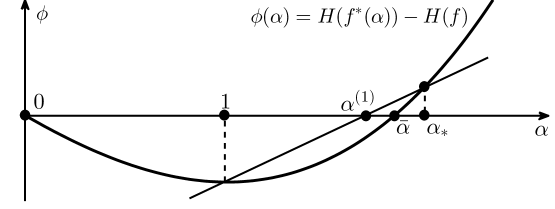
Recall from AK2002jsp that the viscosity relation (2) is derived with . Then should be close to 2 as much as possible in order to maintain the consistency. To this end, we introduce
| (8) |
Notice that near equilibrium. If , then is taken as , which maintains the entropy inequality (7). Otherwise, we refer to Fig. 1 and take
| (9) |
From Fig. 1 we can see that this will be very close to the solution of the entropy balance equation (4) if is small, which is of frequent occurrence. Thanks to the convexity of function , it is proved in the Supplementary Material that
About the above implementation, three remarks are in order. (a). The implementation not only guarantees the nonnegativity of distributions but also maintains the discrete H-theorem (6). The former is due to and the latter follows from or . (b). The introduction of is a key in our implementation, it reduces the computational cost drastically. Indeed, is often much smaller than used in AK2002jsp ; AK2002 ; TUSK2007 ; BGL2007 . It also extracts lots of grid points where the entropy balance (4) is irrelevant. Moreover, our numerical example shows that the number of grid points where is about half of the total grid point number, see Fig. 5. (c). Formula (9) is much simpler than those given in AKTA2017 . It relies neither on any near-equilibrium assumption nor on the specific form of the entropy function , while those in AKTA2017 do.
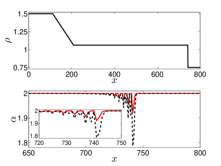
To compare Formula (9) and the essentially ELBM (EELBM) with its first-order approximation AKTA2017 , we simulate the one-dimensional shock tube problem in AK . The exact density profile is displayed in Fig. 2 and the two implementations both produce solutions oscillating near the shock. We see that in a narrow region of the shock front, obtained with the implementations is not larger than 2 and our implementation gives larger than the EELBM. At the point of maximum departure, the deviation of from 2 is 10.71% for the EELBM while that for the present implementation is only 3.96%. This clearly shows that Formula (9) gives a better approximation to the solution of the equation (4) than the first-order EELBM.
Furthermore, we simulate the double shear flow with periodic boundary conditions. For this problem, the spatial domain is , and the initial state is MB1997 ; KBC2014
and . Here and are the and component of the fluid velocity, respectively, and determines the slop of the shear layer.
To show the effectiveness and efficiency of our implementation, we solve this problem with three approaches: our implementation, the first-order EELBM AKTA2017 , and the bisection method used in BGL2007 for the equation (4). The stop criterion for the bisection method is . Here we use the D2Q9 lattice, for which the equilibrium minimizing the entropy (3) has an analytical expression AKO2003 , and the mesh size is taken as . For this setup, the results produced with the three approaches are displayed in Fig. 3.

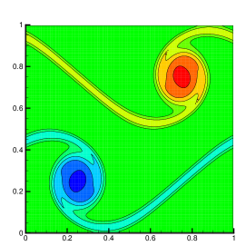
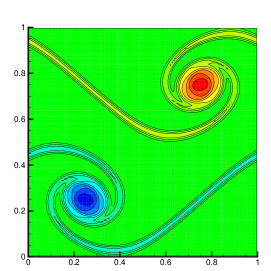
They are the contour lines of vorticity at (, where is the number of time steps and is the mesh size). It can be seen that, except for the EELBM, the other two methods yield almost the same shape of vortex that is consistent with those in MB1997 ; KBC2014 . Furthermore, we also plot the distributions of in Fig. 4 for the three implementations above. It clearly shows that our is smaller than 2 near the vortexes and close to 2 elsewhere.
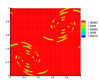
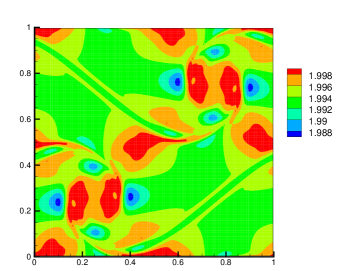
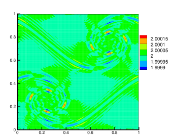
These demonstrate the efficiency of our implementation.
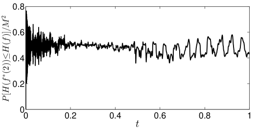
To have a closer look at our implementation, we also count the number, by , of the grid points where at each time step. The proportion as a function of time is plotted in Fig. 5. We see that the proportion is around for most of the time. Namely, at each time step Eq. (4) needs to be solved only for about half of the total grid point number. Therefore, the introduction of in (8) enhances the efficiency significantly.
In conclusion, we have presented a simple and uniform relaxation-rate formula for the ELBM. The formula solves a long-standing critical problem in kinetic theory approach: it not only guarantees the nonnegativity of the distributions and the discrete H-theorem, but also gives full consideration to the consistency with hydrodynamics. We demonstrate that with our new implementation based on the relaxation-rate formula the algebraic equation only needs to be solved for about half of the grid points, where the flow fields change drastically is effectively marked, and the computational overhead of the ELBM is greatly reduced. Thus the novel relaxation-rate formula makes a significant step for the development of the ELBM and now the method can be efficiently used for a broad range of hydrodynamics applications including turbulence flows.
Finally, we point out that Formula (9) can be improved with the following iteration (a modified secant algorithm)
for . In the Supplementary Material it is proved that this iteration converges unconditionally to the solution of Eq. (4) and for all .
References
- (1) S. Succi, The Lattice Boltzmann Equation for Fluid Dynamics and Beyond, Oxford University Press, Oxford, 2001.
- (2) Z. Guo and C. Shu, Lattice Boltzmann Method and its Applications in Engineering, Word Scientific Publishing Company, Singapore, 2013.
- (3) R. Benzi, S. Succi, M. Vergassola, Phys. Rep. 222(3) 145 (1992).
- (4) S. Chen, G. D. Doolen, Ann. Rev. Fluid Mech. 30(1), 329 (1998).
- (5) C. K. Aidun, J. R. Clausen, Ann. Rev. Fluid Mech. 42(1), 439 (2010).
- (6) S. Ansumali, I.-V. Karlin, Phys. Rev.E 62, 7999 (2000).
- (7) B.-M. Boghosian, J. Yepez, P. V. Coveney, A. J. Wagner, Phil. Trans. R. Soc. Lond. A 457, 717 (2001).
- (8) I.-V. Karlin, A.-N. Gorban, S. Succi, V. Boffi, Phys. Rev. Lett. 81:6 (1998).
- (9) I.-V. Karlin, A. Ferrante, H. C. Öttinger, Europhys. Lett. 47, 182 (1999).
- (10) S. Ansumali, I.-V. Karlin, Phys. Rev. E 65, 056312 (2002).
- (11) S. Ansumali, I.-V. Karlin, J. Stat. Phys. 107, 291 (2002).
- (12) S. Ansumali, I.-V. Karlin, H. C. Öttinger, Europhys. Lett. 63, 798 (2003).
- (13) B.-M. Boghosian, P. J. Love, J. Yepez, Phil. Trans. R. Soc. Lond. A 362 1691 (2004).
- (14) S. S. Chikatamarla, S. Ansumali, I.-V. Karlin, Phys. Rev. Lett. 97, 010201 (2006).
- (15) B. Keating, G. Vahala, J. Yepez, M. Soe, L. Vahala, Phys. Rev. E 75, 036712 (2007).
- (16) I.-V. Karlin, F. Bösch, S. S. Chikatamarla, Phys. Rev. E 90, 031302(R) (2014).
- (17) M. Atif, P. K. Kolluru, C. Thantanapally, S. Ansumali, Phys. Rev. Lett. 119, 240602 (2017).
- (18) S. S. Chikatamarla, C. E. Frouzakis, I.-V. Karlin, A. G. Tomboulides, K. B. Boulouchos, J. Fluid Mech. 656, 298 (2010).
- (19) B. Dorschner, F. Bösch, S. S. Chikatamarla, K. Boulouchos, I.-V. Karlin, J. Fluid Mech. 801, 623 (2016).
- (20) A. M. Moqaddam, S. S. Chikatamarla, I.-V. Karlin, J. Stat. Phys. 161, 1420 (2015).
- (21) A. M. Moqaddam, S. S. Chikatamarla, I.-V. Karlin, Phys. Fluids 28, 022106 (2016).
- (22) A. M. Moqaddam, S. S. Chikatamarla, I.-V. Karlin, Phys. Rev. E 92, 023308 (2015).
- (23) N. Frapolli, S. S. Chikatamarla, I.-V. Karlin, Phys. Rev. E 92, 061301(R) (2015).
- (24) F. Tosi, S. Ubertini, S. Succi, I.-V. Karlin, J. Sci. Comput. 30, 369 (2007).
- (25) R. A. Brownlee, A. N. Gorban, J. Levesley, Phys. Rev. E 75, 036711 (2007).
- (26) Y. H. Qian, D. d’Humières, P. Lallemand, Europhys. Lett. 17(6), 479 (1992).
- (27) M. L. Minion, D. L. Brown, J. Comput. Phys. 138, 734 (1997).